The post Disaggregated Scheduled Fabric: Scaling Meta’s AI Journey appeared first on Engineering at Meta.
]]>Disaggregated Schedule Fabric (DSF) is Meta’s next-generation network fabric. The GenAI boom has created a surge in demand for high-performance, low-latency, and lossless AI networks to support training AI models at a large scale. DSF helps us build scalable AI networks by breaking the physical limit of the traditional monolithic chassis-switch architecture. By disaggregating line cards and fabric cards into distinct, interconnected hardware devices, the DSF network creates a distributed system that offers scalability and performance for AI networks.
DSF is a VOQ-based system powered by the open OCP-SAI standard and FBOSS with a modular architecture designed to optimize load balancing and congestion control, ensuring high performance for both intra and inter-cluster traffic.
With DSF we’ve already been able to build increasingly larger clusters that interconnect thousands of GPUs in a data center region.
Background: Our Challenges With Traditional IP Fabric
While running training jobs over traditional IP fabric, we faced several challenges. These problems were specific to training applications that use remote direct memory access (RDMA) technology, which uses UDP protocol to exchange data.
We encountered these three types of problems:
- Elephant flows: AI workloads tend to have long-duration, heavy-traffic flows that have the potential to congest the fabric links they hash onto and create head-of-the-line blocking.
- Low entropy: Depending on the number of GPUs involved in the collective operations, the number of IP flows could be lower, which results in inefficient hashing and, possibly, in congestion, despite the availability of adequate capacity in the fabric.
- Suboptimal fabric utilization: We have observed that, as a combined effect, there is a large skew in the bandwidth utilization of fabric links. This is important data because it impacts how much we should overprovision the fabric to support good pacing and maintain steady performance in the event of failures.
We tried several solutions to handle these issues, but each presented challenges. For example, we created Border Gateway Protocol (BGP) policies such that when traffic is received from accelerators via leaf switches, it is pinned to a specific uplink, depending on its destination. This alleviated the problem of low entropy in steady state but didn’t handle failure scenarios where the fallback was equal-cost multipath (ECMP) routing.
We also tried load-aware ECMP schemes that could handle fat flows and low entropy, but they were difficult to tune and created out-of-order packets, which is detrimental to RDMA communication.
We also created a traffic-engineering solution that would pre-compute the flow pattern depending on the models used and configure the leaf switches before the job starts. This could handle fat flows and low entropy but grew too complex as network size increased. And due to its centralized nature, this set-up was slow to react to failures.
A Primer on Disaggregated Scheduled Fabric
The idea behind DSF stems from the aforementioned characteristics of AI training workloads, particularly their tendency to generate “elephant flows” — extraordinarily large, continuous data streams — and “low entropy” traffic patterns that exhibit limited variation in flow and result in hash collisions and sub-optimal load distribution across network paths. The fundamental innovation of DSF lies in its two-domain architecture, which separates the network into the Ethernet domain, where servers and traditional networking protocols operate, and the “fabric” domain, where packets will be broken into cells, sprayed across the fabric, and subsequently reassembled at the hardware before being delivered back to the Ethernet domain.
DSF is built on two components: interface nodes (INs), also referred to as rack disaggregated switches (RDSWs), and fabric nodes (FNs), known as fabric disaggregated switches (FDSWs). INs serve as the network-facing components that handle external connectivity and routing functions, and that interface with the broader data center infrastructure. FNs operate as internal switching elements dedicated to high-speed traffic distribution across the fabric without requiring Layer 3 routing capabilities.
To the external network infrastructure, this distributed collection of INs and FNs appears as a single, unified switch, with the total number of external ports equivalent to the aggregate of all external ports across all INs, effectively creating a virtual chassis switch that scales far beyond the physical limitations of traditional designs. The control plane that orchestrates this distributed system is built upon Meta’s FBOSS, an open-source network operating system that supports the multi-ASIC control requirements of disaggregated fabrics. Its communication with FBOSS State DataBase (FSBD) enables real-time state synchronization across nodes.
DSF achieves traffic management by packet spraying and a credit-based, congestion control algorithm. Unlike conventional Ethernet fabrics that rely on hash-based approaches, DSF utilizes packet spraying that distributes traffic across all available paths through the fabric. Such a feature is enabled by the hardware’s ability to reassemble packet cells at the interface nodes within the fabric domain while ensuring in-order delivery to end hosts.
This packet-spraying capability is orchestrated through a credit-based allocation scheme where ingress INs dynamically request credit tokens from egress INs, allowing the system to make real-time decisions based on current path availability, congestion levels, and bandwidth utilization. Virtual output queuing (VOQ) helps with ensuring lossless delivery throughout this process, directing incoming packets to virtual output queues targeting specific destination ports and service classes, with each virtual output queue being scheduled independently for transmission, providing fine-grained traffic management that can accommodate the requirements of AI workloads and communication patterns.
This approach allows DSF to achieve near-optimal load balancing across all available network paths, effectively utilizing the full bandwidth capacity of the fabric. It provides the flexibility to handle mixed traffic patterns and adapt to dynamic network conditions without requiring manual reconfiguration or traffic engineering.
DSF Fabric for GenAI Applications
DSF Fabric (GenAI)
Using the DSF technology, we built a massive cluster that interconnects thousands of GPUs within a data center region. Figure 1 illustrates the network topology of a single AI zone that is a building block for the larger cluster.
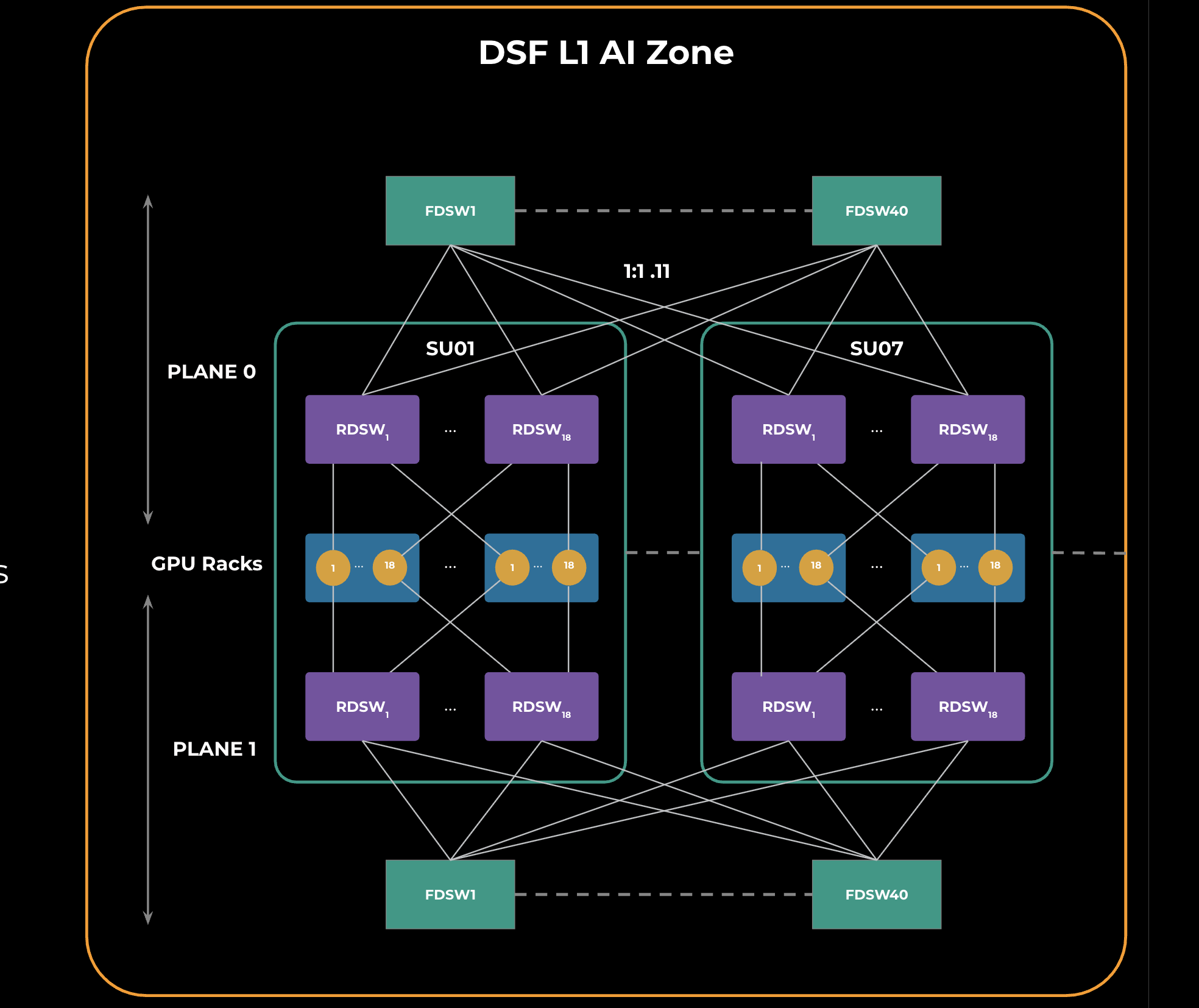
An AI zone contains multiple scaling units, shown in Figure 1 as “SUx.” A scaling unit is a grouping of GPU racks connected to RDSWs within the scaling unit. All the RDSWs within the AI zone are connected via a common layer of FDSWs. RDSWs are powered by deep-buffer Jerico3-AI chips, while FDSWs use Ramon3 chips. FBOSS is the network operating system for all the roles in this topology. We are using 2x400G FR4 optics between RDSW-FDSW connections.
The GPU to RDSW connections are rail optimized, which benefits hierarchical collectives like allreduce and allgather, both of which are latency sensitive.
To support high GPU scale in a single AI zone, two network planes that are identical to each other are created. This is called a DSF L1 zone and is a building block for larger GenAI clusters, as we will see in the next section.
DSF Dual-Stage Fabric (GenAI)
As depicted in Figure 2 (below) we interconnected 4x DSF L1 zones through a second stage of spine DSF switches (SDSWs). SDSWs use the same hardware as FDSWs and aggregate DSF L1 zones, enabling them to act as a single DSF fabric. This is a non-blocking topology providing an interconnected GPU scale of 18K x 800G GPUs.

All RDSWs in this topology maintain fully meshed FDSB sessions to exchange information such as IPv6 neighbor states. There is also an innovative feature — input-balanced mode — enabled over this fabric to smartly balance the reachability info across the layers such that, in case of failures, congestion is avoided over the fabric and spine layer. This feature will be explained in a separate section below. We call this topology the DSF L2 zone.
DSF Region (GenAI)
To achieve a larger interconnected GPU scale, we connected 5x DSF L2 zones via the L3 super-spine layer. (See Figure 3 below.) We did this by using a special edge point of delivery (PoD) in each of the buildings. Edge PoDs consist of 40 FDSWs and 128 edge DSF switches (EDSWs). From a hardware point of view, EDSW is the same as RDSW but differs in its function of providing connectivity to the L3 super spine.
Each EDSW connects to four superspine devices using 4x800G links provisioning a total of 2k x800G ports per edge PoD.
The way training models are sharded we don’t expect a lot of traffic transiting the L3 super-spine layer; hence, an oversubscription of 4.5:1 is sufficient.
This creates an L3 interconnect, which means we need to exchange the routing information. We created iBGP sessions with EDSW and all RDSWs within the building, with BGP add-path enabled such that RDSWs learn aggregates via all 2k next-hops.
eBGP is used between EDSW and the L3 super spine, and only aggregates are exchanged over BGP peerings.
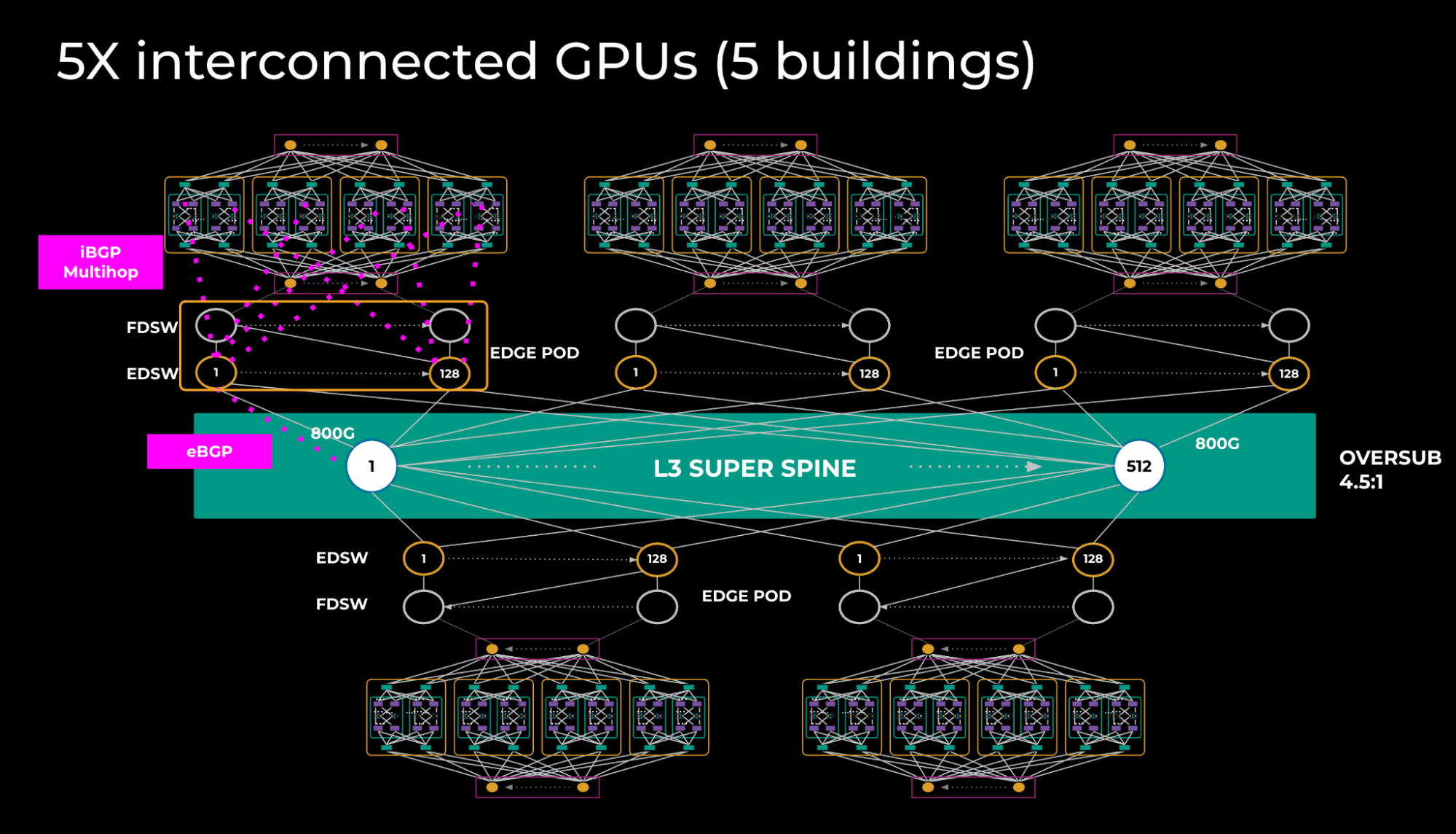
Given that L3 spine is used, some of the problems, including entropy and fat flow, tend to reappear; however, at this network tier where there’s much less traffic, those problems are less profound.
Input Balanced Mode
Input Balanced Mode is a critical feature that supports balanced traffic throughout the network in the face of remote link failures. The feature avoids severe congestion on the fabric and spine layer of the DSF network.
Mechanism
The purpose of Input Balanced Mode is to ensure any DSF devices have equal or less input BW compared to output BW. No oversubscription should occur in the network, even in the case of remote link failure. Devices experiencing link failure will propagate the reduced reachability information across the cluster, notifying other devices to send proportionally less traffic to the affected device.
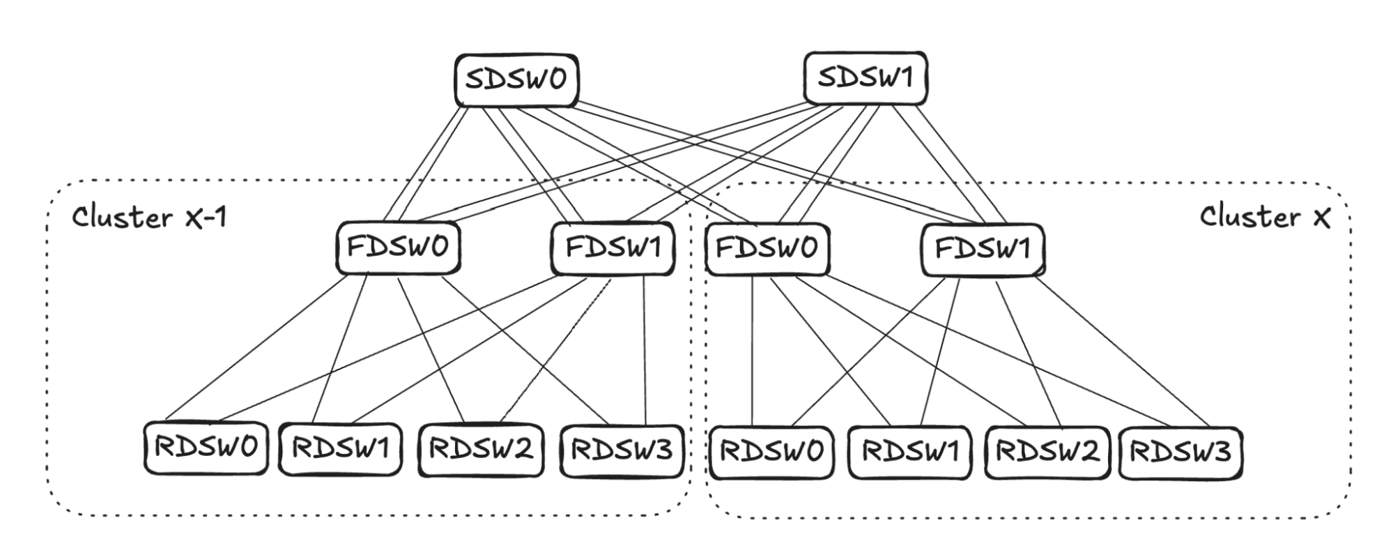
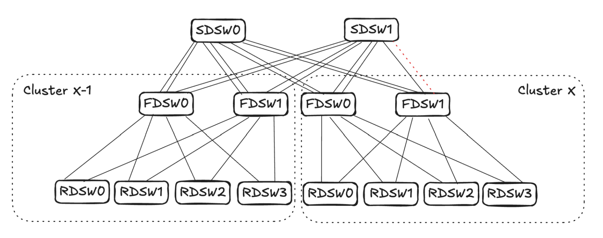
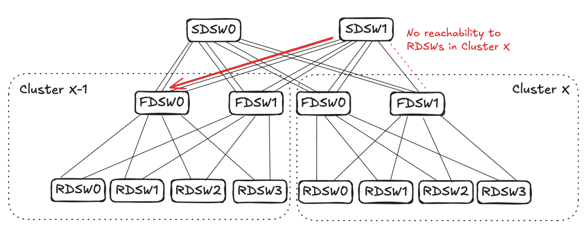
Note: For clarity, in Figure 4, FDSW/SDSW are simplified to only show one virtual device. The above graph will be used to illustrate two different link failures and mechanisms.
RDSW<->FDSW Link Failure
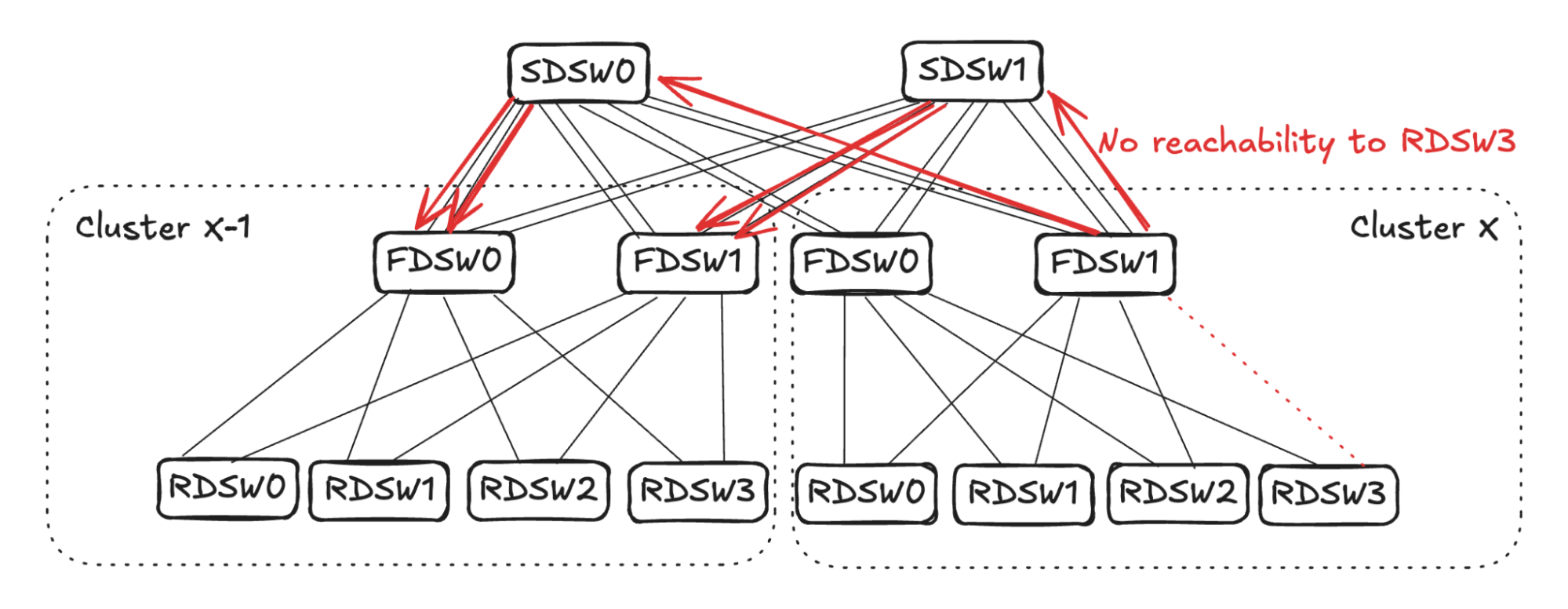
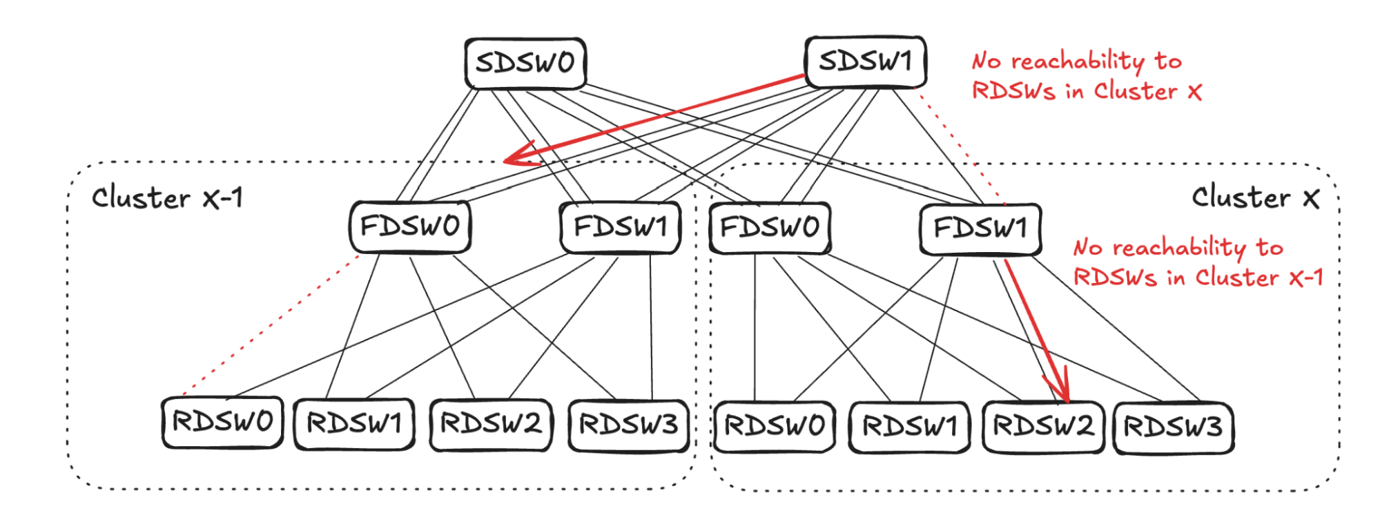
In the case of RDSW<->FDSW link failure, RDSW will lose connectivity to the FDSW, hence losing both input and output capacity on the link. FDSW also loses connectivity to the RDSW and then stops advertising the connectivity. In Figure 5 (below) FDSW1 in Cluster X loses connection to RDSW3, hence it stops advertising reachability to SDSW0 and SDSW1.
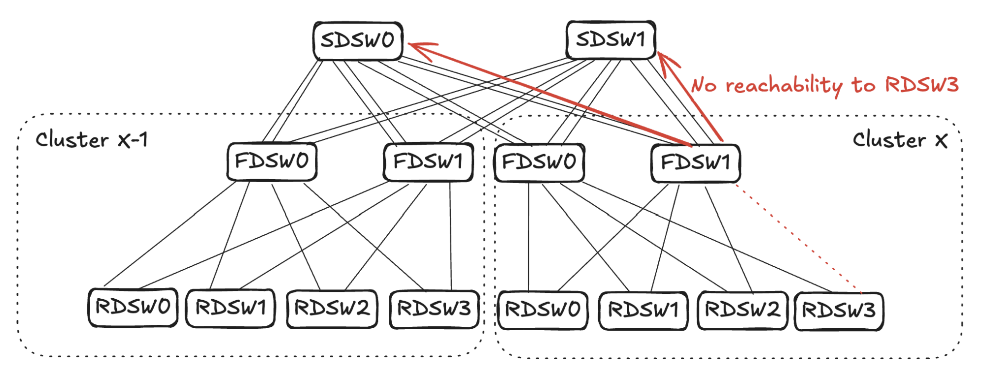
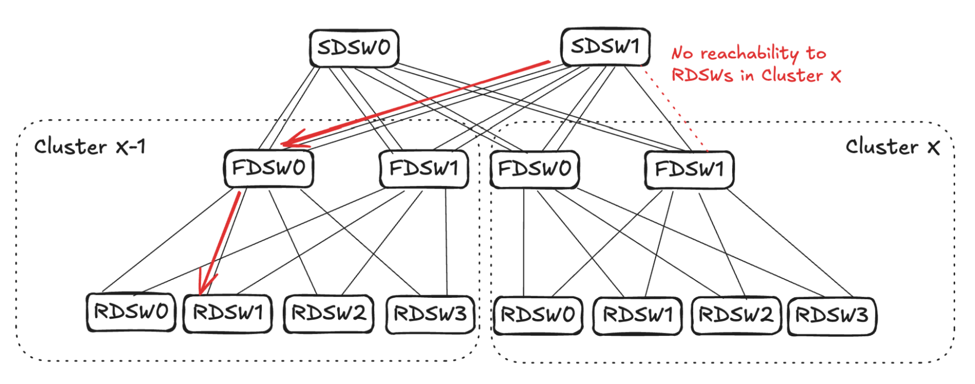
From SDSW0’s perspective, it receives no reachability to RDSW3 from FDSW1 in Cluster X, but still has reachability to RDSW3 through FDSW0. (See Figure 6.) Toward destination RDSW3 in Cluster X, the input capacity of 4 (FDSW0 and FDSW1 from Cluster X-1) is greater than the output capacity of 2 (FDSW0 in Cluster X). To avoid oversubscription, SDSW0 will pick two input links and stop advertising reachability toward RDSW3 in Cluster X. The same sequence will also take place in SDSW1.
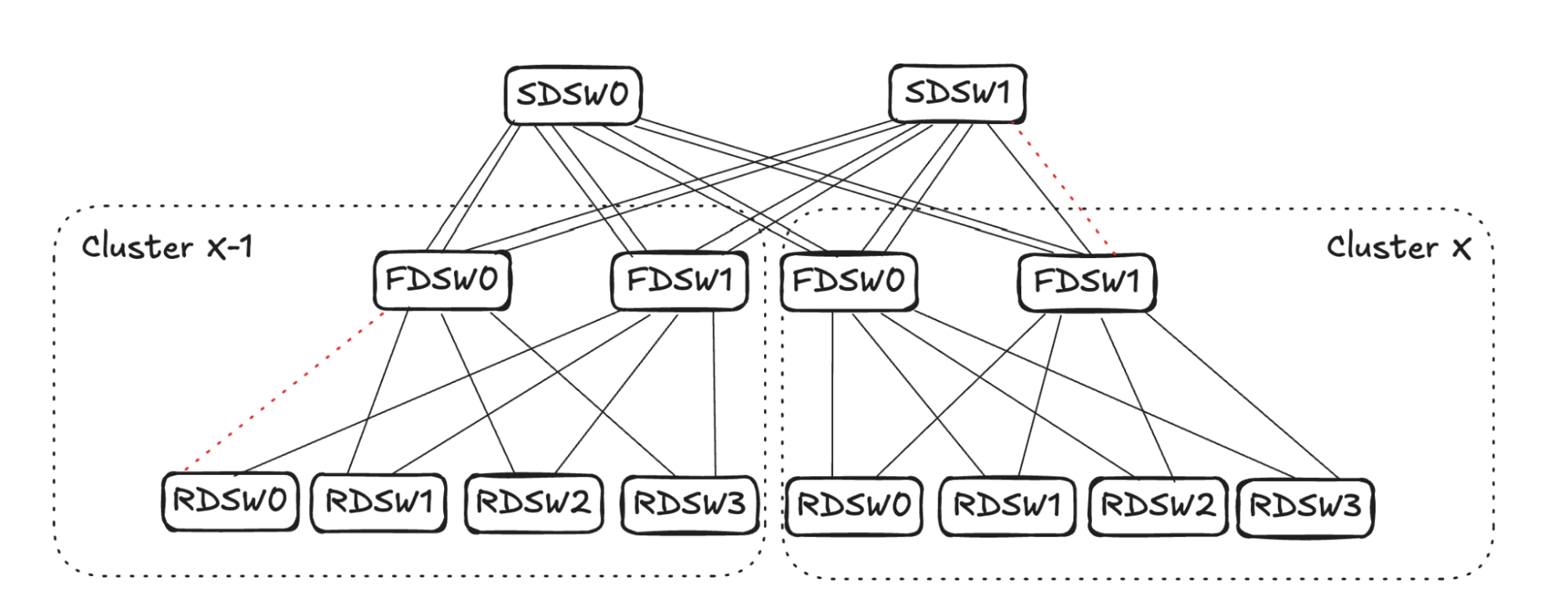
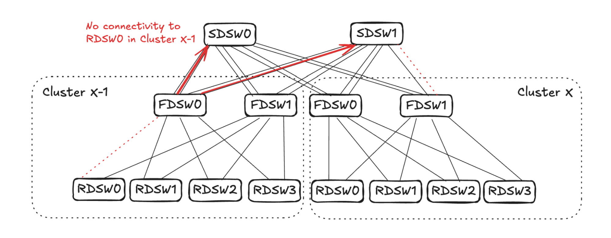
The link selection for balanced input mode should be randomized. As shown in Figure 7 (below), for simplicity’s sake, assume SDSW0 stops advertising reachability to FDSW0, and SDSW1 stops advertising reachability to FDSW1. Both FDSW0 and FDSW1 have an input capacity of 4 but an output capacity of 2, hence randomly selecting two links on each device to not advertise reachability.
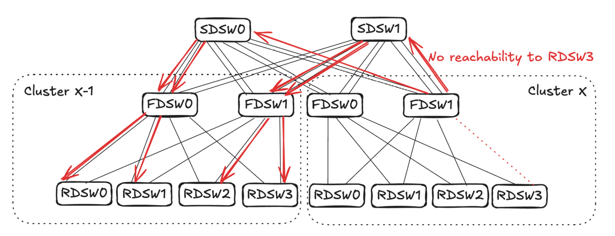
Assume FDSW0 randomly selects links to RDSW0 and RDSW1, while FDSW1 randomly selects links to RDSW2 and RDSW3. This completes the propagation of link failure, resulting in RDSWs in Cluster X-1 having 50% capacity to forward traffic toward RDSW3 in Cluster X.
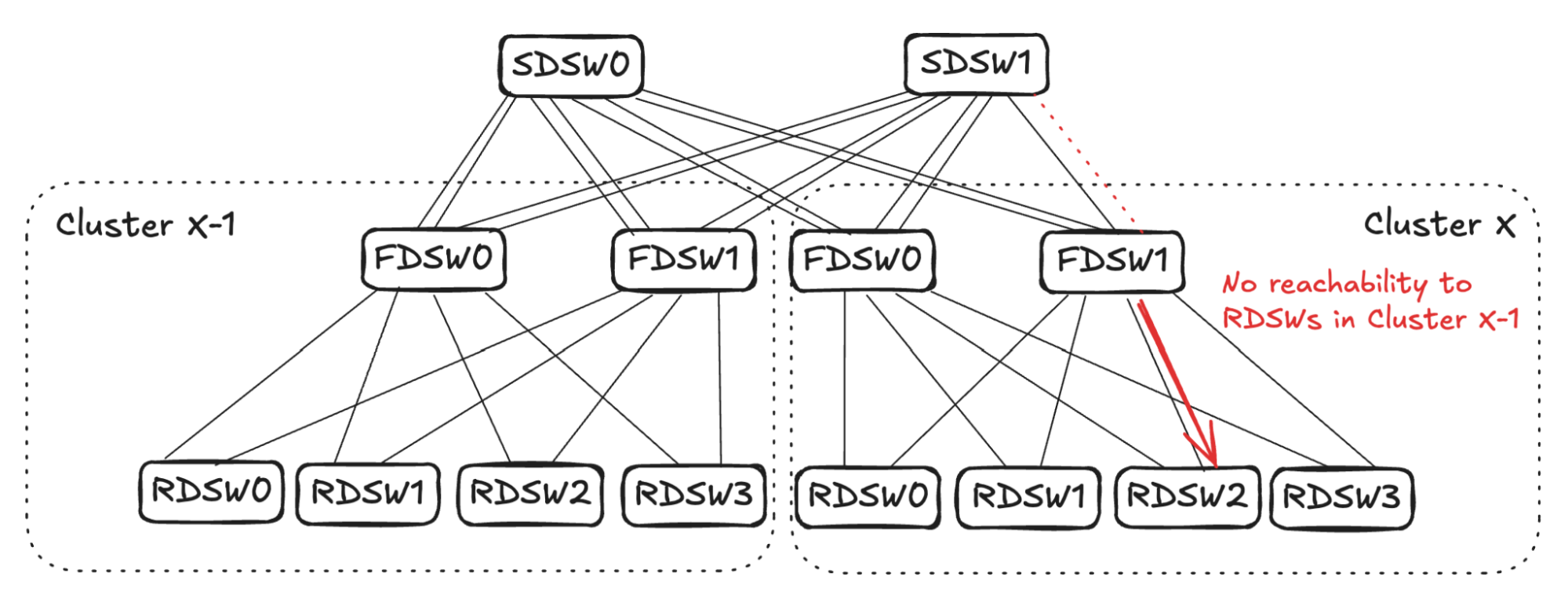
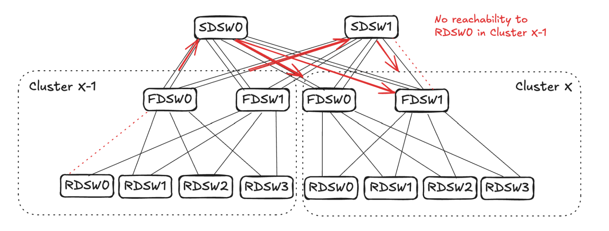
FDSW<->SDSW Link Failure
Upon FDSW<->SDSW link failure, there are two directions to propagate the reduced capacity: 1) on FDSW, reduce input capacity from RDSW, and 2) on SDSW, reduce input capacity from FDSWs in other clusters. (See Figure 8)
FDSW Propagation
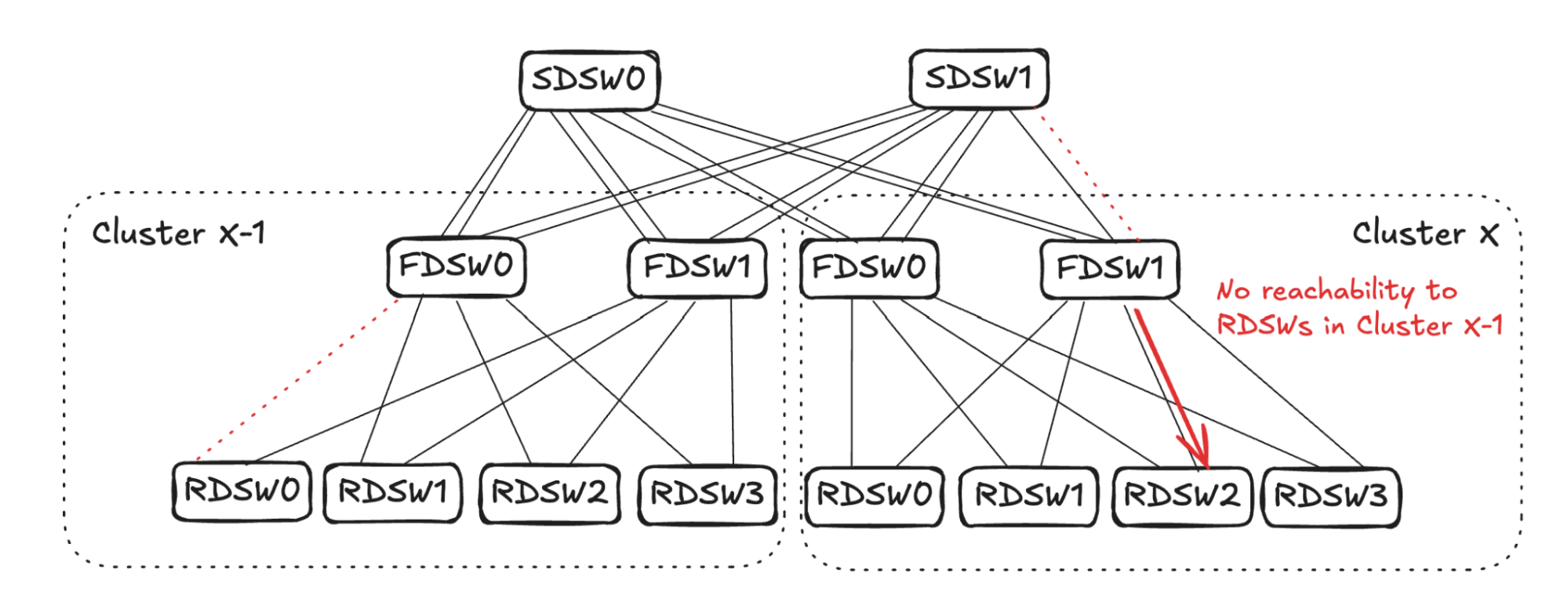
Consider the traffic egressing out of Cluster X thru FDSW1 (see Figure 9): From FDSW1’s perspective, input capacity is 4 (from RDSW0-RDSW3) while output capacity is reduced to 3 due to link failure.
To balance input capacity, FDSW1 will randomly pick one FDSW<->RDSW link to stop advertising reachability to ALL destinations outside of the cluster.
Assume Cluster X FDSW1 randomly picks the link to RDSW2. It will stop advertising reachability to all RDSWs in Cluster X-1. Note that the same link can still be utilized for intra-cluster traffic, as it has full reachability to RDSWs in Cluster X.
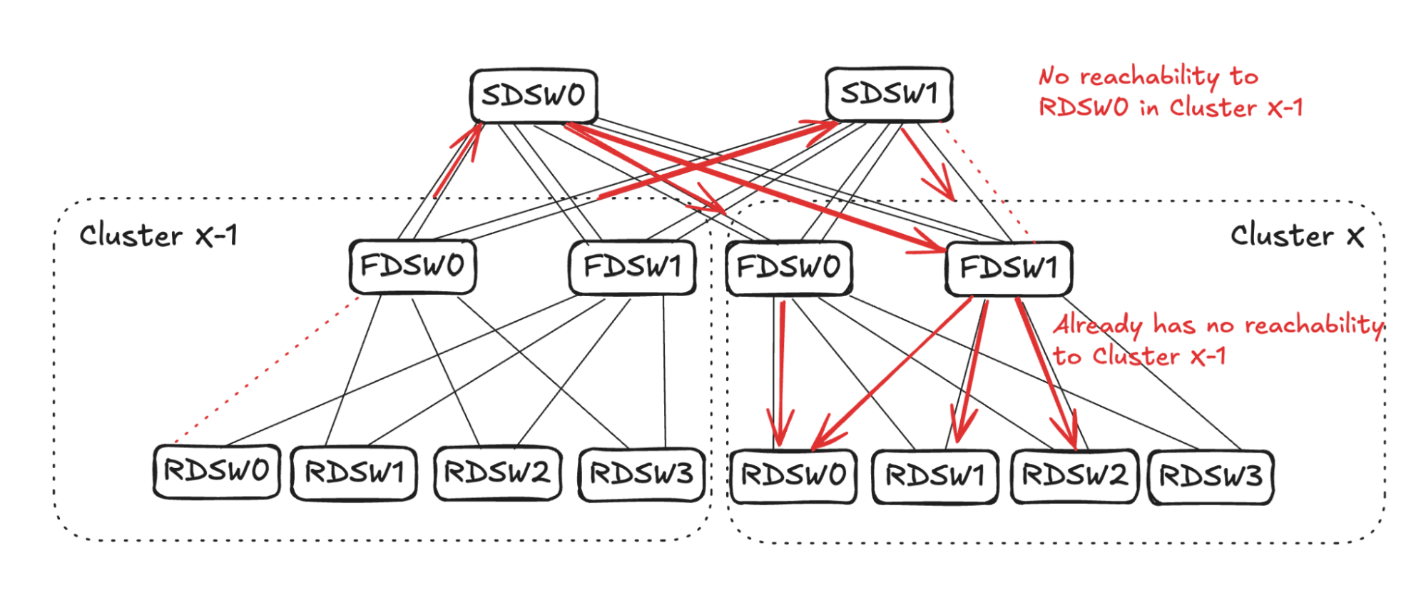
SDSW Propagation
Consider traffic ingressing into Cluster X thru SDSW1 (see Figure 10): From SDSW1’s perspective, input capacity is 4 (from FDSW0 and FDSW1 in Cluster X-1), while due to link failure, output capacity is 3. SDSW1 will randomly pick one link towards Cluster X-1 and stop advertising reachability to all RDSWs in Cluster X.
A similar calculation will take place on FDSW0 in Cluster X-1, resulting in Cluster X-1 FDSW0 randomly picking one link and stopping advertising reachability to all RDSWs in Cluster X. (See Figure 11 below) This completes the propagation, leading to RDSW1 in Cluster X-1 losing one link to forward traffic toward Cluster X.
FDSW<->SDSW and RDSW<->FDSW Link Failure
Figure 12 illustrates another example of link failures occurring in between FDSW <-> SDSW, as well as RDSW <-> FDSW. The reduced reachability will propagate and then converge in both directions.
- FDSW<->SDSW link failure.
- RDSW<->FDSW link failure.
FDSW Propagation for FDSW<->SDSW Link Failure
Similar to the above FDSW propagation, FDSW1 in cluster X will randomly pick one connecting RDSW and advertise no reachability to devices towards Cluster X-1. (See Figure 13 below)
SDSW propagation for FDSW<->SDSW Link Failure
Similar to the SDSW propagation above, SDSW1 will randomly pick one link towards cluster X-1 and propagate no reachability to Cluster X. Imagine SDSW1 picks one of the links connecting FDSW0 in cluster X-1.
Note in Figure 14 that FDSW0 in Cluster X-1 already has one link failure connecting RDSW0. The input and output capacity towards Cluster X is already balanced on FDSW0, thus finishing propagation in this direction.
FDSW Propagation for RDSW<->FDSW Link Failure
As FDSW0 in Cluster X-1 loses connectivity to RDSW0, it will stop advertising reachability to SDSW0 and SDSW1 on both of the links. (See Figure 15.)
SDSW0 will randomly pick two links to stop advertising reachability to RDSW0 in Cluster X-1 (in the example in Figure 16 it picks one link in FDSW0 and one in FDSW1). On SDSW1, however, it already has one link failure connecting FDSW1 in Cluster X. Therefore, only one more link needs to be selected to propagate the reduced reachability (in the example it picks the other link towards FDSW1).
From Cluster X FDSW1’s perspective, the output capacity towards RDSW0 in Cluster X-1 is 1 (two links with no reachability, and one link failure). Therefore, to balance input it should select three links to stop advertising reachability towards RDSW0 in Cluster X-1. Note that the link FDSW1<->RDSW2 already has no reachability towards Cluster X-1 due to 1.1 propagation above. Hence, it will pick two more links (RDSW0 and RDSW1 in Figure 17) to not advertise reachability.
For Cluster X FDSW0, it will randomly pick one downlink (RDSW0 in Figure 17) to not advertise reachability to RDSW0 in Cluster X-1.
Future Work With DSF
- We are interconnecting multiple regions to create mega clusters that will provide interconnectivity of GPUs with different regions that are tens of kilometers apart.
- This will create an interesting challenge of addressing heterogeneity between different GPU types and fabric involving different regions.
- We are also working on a new technology called Hyperports, which will combine multiple 800G ports at ASIC level to act as a single physical port. This will reduce the effect of fat flows on IP interconnects.
In addition, DSF is a smart fabric that inherently supports a wide range of GPUs/NICs. We are increasing our deployments to include an increasing variety of GPU/NIC models.
The post Disaggregated Scheduled Fabric: Scaling Meta’s AI Journey appeared first on Engineering at Meta.
]]>The post Scaling LLM Inference: Innovations in Tensor Parallelism, Context Parallelism, and Expert Parallelism appeared first on Engineering at Meta.
]]>The rapid evolution of large language models (LLMs) has ushered in a new era of AI-powered applications, from conversational agents to advanced content generation. However, deploying these massive models at scale for real-time inference presents significant challenges, particularly in achieving high throughput, low latency, and better resource efficiency.
Our primary goal is to optimize key performance metrics:
- Resource efficiency: Maximizing GPU utilization to improve operational efficiency.
- Throughput (queries/s): Serving more users by processing a higher volume of requests.
- Latency: Minimizing response times for a seamless user experience. This includes:
- Time-to-first-token (TTFT) for prefill: The time it takes for the first part of the response to appear, ideally under 350ms.
- Time-to-incremental-token (TTIT) for decoding: The latency between subsequent words, targeting less than 25ms.
These metrics highlight the distinct computational demands of LLM inference: Prefill is compute-intensive, while decoding is memory bandwidth-intensive. To address these challenges and enable the deployment of large models, we have developed and implemented advanced parallelism techniques.
The Two Stages of LLM Inference
A typical LLM generative-inference task unfolds in two stages:
- Prefill stage: This stage processes the input prompt (which can be thousands of tokens long) to generate a key-value (KV) cache for each transformer layer of the LLM. Prefill is compute-bound, because the attention mechanism scales quadratically with sequence length.
- Decoding Stage: This stage utilizes and incrementally updates the KV cache to generate tokens (words) one by one. Decoding is memory-bound, as the I/O time of reading memory dominates attention time, with model weights and the KV cache occupying the majority of memory.
Addressing Bottlenecks With Parallelism
To scale LLM inference effectively, especially for handling long contexts and massive models, we employ three main types of inference parallelism:
1. Tensor parallelism (TP), which improves fitting large models across multiple GPUs and achieving high throughput that a single device cannot provide. It involves sharding individual layers of the model, such as attention blocks and multi-layer perceptron (MLP) layers, into smaller, independent blocks that can be executed on different devices.
A challenge in tensor parallelism is the “allreduce” communication operation, which can contribute up to 30% of end-to-end latency. To mitigate this, we developed direct data access (DDA) algorithms:
- DDA flat algorithm: Improves small message-size allreduce latency by allowing each rank to directly load memory from other ranks and perform local reduce operations. This reduces latency from O(N) to O(1) by increasing the amount of data exchange from O(n) to O(n^2).
- DDA tree algorithm: Breaks the allreduce into two phases (reduce-scatter and all-gather) and uses direct data access in each step. This moves the same amount of data as the ring algorithm but reduces latency to a constant factor, making it suitable for slightly larger message sizes.
Our DDA solutions demonstrate significant speedups against baselines such as NCCL (NVIDIA Collective Communications Library) and RCCL (ROCm Communication Collectives Library for AMD GPUs). For instance, with AMD MI300X, we achieved overall performance parity with Nvidia H100, with DDA outperforming RCCL baseline by 10-50% for decode (small message sizes) and yielding 10-30% speedup for prefill, resulting in approximately 10% reduction in TTIT.
2. Context parallelism (CP), which facilitates managing and processing extremely long contexts, such as the 1M/10M token capabilities introduced with Llama 4. Long-context inference presents unique challenges:
- Compute: Dense attention FLOPs scale quadratically with context length, leading to attention-compute dominating.
- Memory: The KV cache grows linearly with context.
- Communication: Communication latency increases when parallelizing across multiple hosts.
We have implemented two variants of context parallelism in the attention module, often referred to as “ring attention”:
- Pass-KV: In this approach, input tokens are split across multiple CP ranks. Each rank calculates its portion of query, key, and value tensors. Then, key and value tensors are exchanged between ranks to enable attention interactions across the full context.
- Pass-Q: Similar to Pass-KV, but query tensors are exchanged between ranks.
Our context parallelism optimizations, combined with a fast-attention kernel, have enabled remarkable performance for long-context capabilities. We achieved less than one minute for one million tokens on a single H100 host and less than one minute for 10 million tokens using distributed inference across multiple H100 hosts (e.g., 32 H100 hosts). With Llama 3 405B, we demonstrated near-linear scaling, achieving 128K token prefill in 3.8 seconds with CP over 16 nodes, and 1M-token prefill in 77 seconds.
3. Expert parallelism (EP), which helps with scaling mixture-of-experts (MoE) models, where a large number of “experts” (neural network modules) make it impossible to fit the entire model onto a single host. In EP-based inference, we utilize a two-shot, all-to-all communication pattern to exchange tokens between data parallelism and expert parallelism ranks based on routing.
The all-to-all communication can contribute 10-30% to end-to-end latency, especially for decode messages (100KB to 2MB). To optimize this, we are exploring solutions including:
- Dynamic all-to-all: Sending sub-chunks of data to remote neighbors.
- Persistent all-to-all: Addressing slowdowns primarily caused by memory-handle exchange, network-load balancing, and CPU overhead.
Looking Ahead: Disaggregated Inference and Future Challenges
To further optimize LLM inference, we are moving towards N-D parallelism (CP, PP, EP, TP across nodes, with separate DP) and disaggregating prefill and decoding tiers. This allows for better resource balancing and the potential to use heterogeneous hardware, where compute-heavy hardware is used for prefill and memory bandwidth-heavy hardware for decoding. This multi-dimensional parallelism can help unblock the serving and evaluation of colossal models.
Future challenges in this space include:
- Cloud fabric design: Optimizing the underlying cloud infrastructure for LLM workloads.
- Communication going to kernel (fused kernel): Integrating communication operations directly into computational kernels for greater efficiency.
- Device-initiated kernel: Enabling devices to initiate operations directly, reducing CPU overhead.
These advancements in parallelization and system-level improvements have helped enable the next generation of AI applications and push the boundaries of what LLMs can achieve. We are committed to continuous innovation to ensure efficient and scalable LLM inference for millions of users worldwide.
The post Scaling LLM Inference: Innovations in Tensor Parallelism, Context Parallelism, and Expert Parallelism appeared first on Engineering at Meta.
]]>The post Branching in a Sapling Monorepo appeared first on Engineering at Meta.
]]>After the conference, we designed, implemented, and open sourced our monorepo branching solution in Sapling. While the code is already open source, in this article we share learnings on:
- How we resolved scalability and developer experience tradeoffs in the design and implementation.
- What problems it solved.
- What feedback we received from other developers at Meta.
The key technical insight is that two workflows — non-mergeable full-repo branching and mergeable directory branching — solved all of the branching-related problems for a large and diverse set of products built at Meta.
We hope that the Sapling open source code and the learnings shared in this article will benefit the wider industry and open source communities.
How Source Control Is Handled at Meta
At Meta, our engineering teams work within a large monorepo with a single main branch. This approach enables unified dependency management, large-scale refactoring, easier collaboration, and code reuse across projects. However, this approach introduces challenges for teams that must manage multiple versions of their code.
In multi-repo setups, teams can rely on repository branches to manage different versions. Source control gives them tools, like cherry-pick and merge, that let them manage the differences between the versions.
In the monorepo, however, repository branches do not work as well for this. Branches affect the whole repository, so creating a branch means unrelated projects and dependencies will remain frozen, and quickly become stale.
In this article we refer to whole repository branching as full-repo branching. What we learned is that for workflows that do not require merging back to the main branch (e.g., product releases where the branch ceases to exist after the release completes and the development moves back to the main branch) full-repo branching is a good solution. In Sapling, this workflow is well supported with the sl bookmark family of commands.
However, for product development workflows where merging back to the main branch is required, we learned that full-repo branching is not a scalable approach. This is because full-repo merges create merge commits with multiple parents, making the commit graph wide (high branching factor) and non-linear. In large monorepos, this creates performance problems for operations like sl log and sl blame. Maintaining a linear commit graph,where most commits have a single parent, is crucial for keeping these operations fast for all monorepo users, not just those utilizing branches.
The core limitation is that full-repo branches are all-or-nothing. If you need to patch a legacy version, or maintain a custom variant for a particular project, you cannot create a branch for the part that you own. Branching forks everything.
A common pattern when attempting to solve this problem was for teams to make multiple copies of their code. However, by doing this they lose a lot of the standard developer tools for managing their branches. This resulted in duplicated effort and error-prone copying of patches between directories.
Directory Branching: Sapling’s Monorepo Branching Solution
To solve these challenges, we have introduced a new set of source control tools in Sapling that can be used to implement a new kind of branching: directory branching. This bridges the gap between using multiple repository branches and maintaining copies of code as separate directories.
With these tools, you are able to treat directories in the monorepo much like traditional repository branches. You create branches by copying the code, maintain the code by cherry-picking, and merging changes between directories as if they were branches, and look at the history of each directory in the context of the copies and merges that were made.
Crucially, while directory branches support merging between directories, at the level of the monorepo’s commit graph, they appear as linear commits. This resolves the scalability challenge with the repo-level merge commits and still provides merging workflows at the directory level.
How Directory Branching Is Implemented in Sapling
Directory branching in Sapling is implemented using a series of operations centered around the sl subtree command.
To branch a directory, you use the sl subtree copy command to copy a directory (or file), either at the current version or from any historical version, to a new location in the repository. Sapling records metadata in the commit that tracks the source directory, source revision, and copy relationship, which allows us to recover the complete history of all files in the new branch. If the code you want to branch is not in the monorepo yet, you can use sl subtree import to create a directory branch of an external repository branch.
Once you have a directory branch, you can use sl subtree graft and sl subtree merge to cherry-pick or merge changes between directory branches. These operations use the stored copy/merge metadata to reconstruct the relationship between directories, enabling Sapling to perform three-way merges between directory branches. The merge algorithm finds the common ancestor of the two directory branches (using the copy metadata) and performs a standard three-way merge, just as it would for regular repository merges, but scoped to the specific directory content.
The Build System and Wider Developer Tooling Integration
An advantage of this approach is that the latest versions of all directory branches are visible at the same time. This means continuous integration (CI) can test against multiple branches with a single checkout, and you can be confident that there are no hidden old branches that are unexpectedly still in use.
At Meta we use Buck2 as our build system. When a component depends on another component that uses directory branching, we use Buck config modifiers (i.e., buck build with the -m flag) to allow us to select which branch is being used.
One downside of directory branching is that code searches can result in multiple hits for each of the branches. It is relevant that the searched-for code appears in multiple places, however it can be difficult to look through the results from multiple branches if they are mingled together. Code search systems capable of ranking results can resolve this issue.
User Feedback on Directory Branching
The introduction of directory branching has been a success, with a large and diverse set of engineering teams within Meta adopting it to manage multiple versions of code. Some teams have also found it useful to temporarily freeze the majority of the monorepo for development stability by remaining on an old commit and using directory branching to merge in changes for specific projects, effectively combining both full-repo branching and directory branching workflows.
We observed the following three common themes of valid reasons for adopting directory branching:
1.) When CI is prohibitively expensive or changes could cause major disruptions. Some teams at Meta used directory branches to effectively separate development and production versions of the code, giving them more control over when their code changes are deployed to production.
2.) Experimental changes where a large number of developers are collaborating over several months, but the changes have the potential of disrupting the production version. At the same time, the collaboration scale is large enough that using a very large stack of diffs to simulate a branch is not practical.
3.) Unblocking migrations from Git. Even if the ultimate goal is to have only one or a few versions in the Sapling monorepo, during the migrations we need an equivalent to Git branches so that the migration can complete and consolidation can take place within the monorepo. It is not always possible to consolidate all branches in Git before migrating to monorepo.
It is worth noting that having a single version of code remains the default assumption for the monorepo. However, if any of the three reasons above apply, directory branching can be used as a solution, providing branching workflows without sacrificing the benefits of a monorepo.
Future Work With Directory Branching
We are also planning to leverage directory branching for better integration of Git repositories into the Sapling monorepo. More specifically, we are developing a lightweight repository migration mechanism. Instead of making an irreversible decision of committing all of the Git repository commits into the monorepo history, we create a soft link to an external repository where Sapling can load the Git history on the fly when the user requests it. This lowers the barrier of entry of Git repositories into the monorepo and is useful for integrations before committing to migrating full history. This will be provided as an option to the sl subtree import command when working with external Git repositories.
Stay tuned—we will publish a separate article on this topic once we have enough learnings to share.
To learn more about Meta Open Source, visit our website, subscribe to our YouTube channel, or follow us on Facebook, Threads, X, Bluesky and LinkedIn.
Acknowledgements
Multiple people at Meta’s Source Control, Developer Experience and Open Source organisations contributed to the design and implementation of directory branching in Sapling. We would like to thank: Chris Cooper, George Giorgidze, Mark Juggurnauth-Thomas, Jon Janzen, Pingchuan Liu, Muir Manders, Mark Mendoza, Jun Wu, and Zhaolong Zhu.
We are also grateful to the Git, Mercurial, and Jujutsu open source communities for their branching-related discussions at the GitMerge 2024 conference in Berlin. We hope that the Sapling open source code and the learnings shared in this article will benefit all source control systems.
The post Branching in a Sapling Monorepo appeared first on Engineering at Meta.
]]>The post 10X Backbone: How Meta Is Scaling Backbone Connectivity for AI appeared first on Engineering at Meta.
]]>Meta’s Backbone network is composed of a set of interconnected routing platforms and provides WAN (wide area network) connectivity among network locations. Meta has architected Backbone in two different networks: Classic Backbone (CBB) and Express Backbone (EBB). They differ in some fundamental ways.
CBB is used to achieve global reach from data centers (DCs) to our points of presence (POPs) where we connect with external carriers. CBB is flexible: It can shrink or grow to support a diverse set of geographies and accommodate a broad range of connectivity requirements. It uses traditional IP/MPLS-TE (Internet Protocol/Multiprotocol Label Switching/Traffic Engineering) technologies.
EBB, in contrast, is built to provide scalable DC-to-DC interconnection. EBB is less flexible, having a sizable minimum installation. It runs a heavily customised stack of software, such as the Open/R routing protocol, and an in-house traffic-engineering stack with onbox agents and a centralized controller.
While we see growth in both networks, it’s EBB that presents the most challenging scalability problems.
In the rest of this post, we will focus on EBB and describe how we actually addressed EBB’s growth and the resulting challenges.
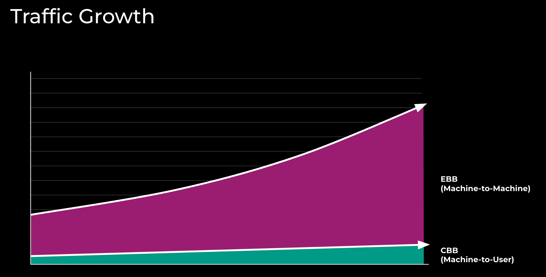 Figure 1: Traffic growth in Meta’s Backbone network
EBB network first started serving traffic around 2015. Figure 1 represents the growth since then for EBB, DC-to-DC traffic flows versus CBB, and DC-to-POP traffic flows.
Prior to 2015, CBB was used for both DC-to-DC and DC-to-POP traffic. Figure 2 represents some of the EBB adoption and technology milestones.
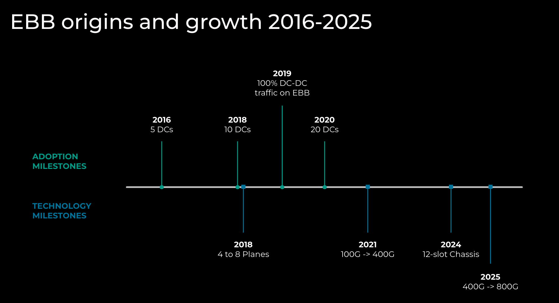 Figure 2: EBB origins and growth
A significant amount of fiber in terms of quantity and distance is required to interconnect DC locations at the necessary scale. The existing DCs continue to grow in footprint and capacity due to the addition of more powerful servers and, where possible, the addition of new buildings at existing locations.
Connecting DCs reliably and repeatedly at high capacity to the rest of the network can be challenging, especially due to the speed at which new DCs are being built. While the network has some input into the site-selection process, there are many influencing factors beyond ease of connectivity that determine how new data center locations are chosen.
10X Backbone
10X Backbone is the evolution of EBB in terms of scale, topology, and technology. Below are the three techniques used to scale to 10X Backbone.
DC Metro Architecture
Historically, building long-haul fibers to new DC locations has been painful, especially when these long-haul fibers need to extend hundreds of miles.
Our first technique to scale up to 10X Backbone was to pre-build some of the components of DC metro architecture. By pre-building them, we could more quickly provide connectivity to new DCs.
First, we built two rings of fiber to provide scalable capacity in the metro, and we connected long-haul fibers to the rings. Next, we built two POPs to provide connectivity toward remote sites. Last, we connected DCs to the rings, and therefore increased or enabled capacity between the DC and POPs. (See Figure 3.)
DC metro architecture has several advantages:
- A simplified building of DC connectivity and WAN topology
- A standardized scalable physical design
- Separate metro and long-haul networks
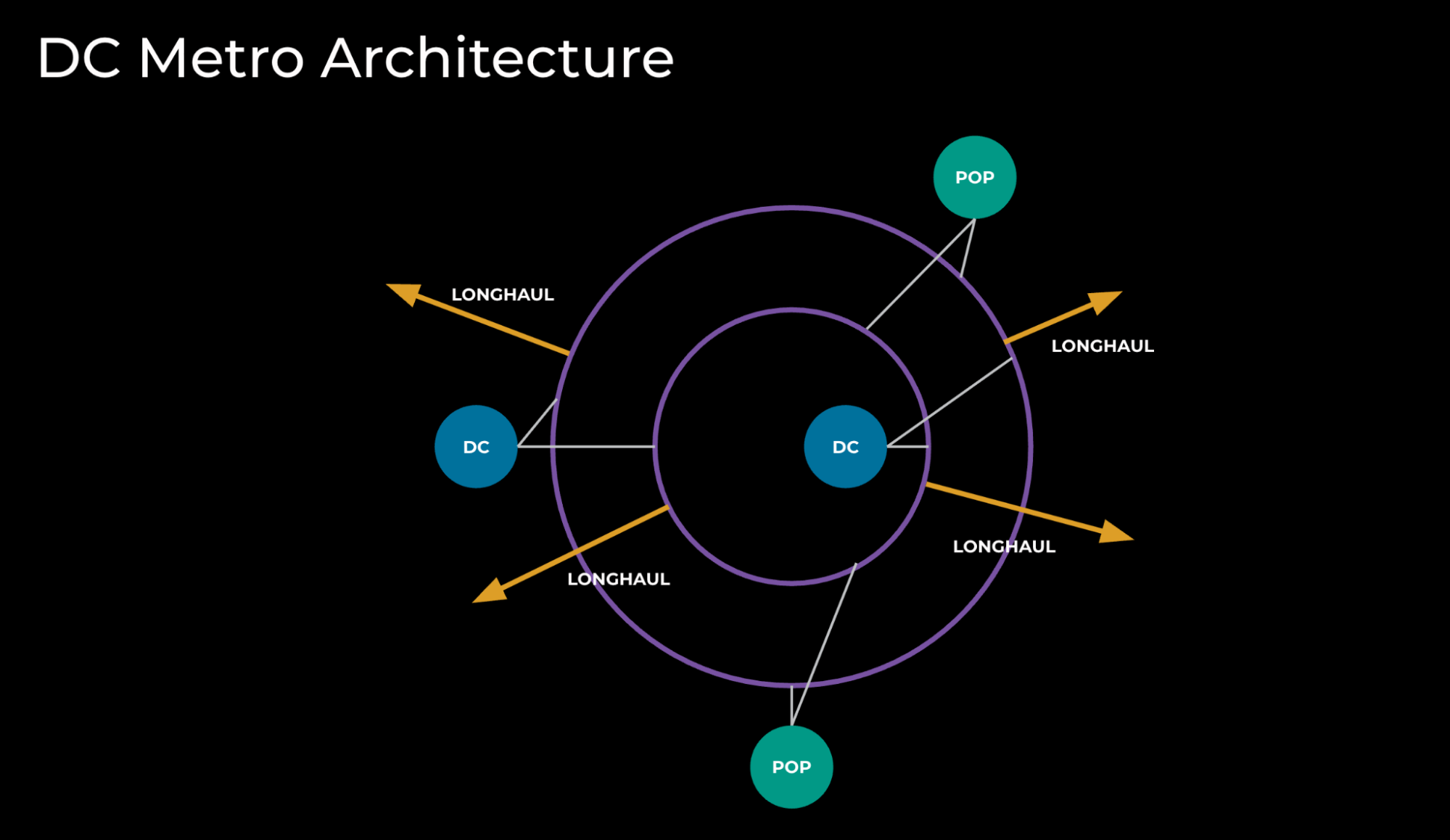 Figure 3: DC metro architecture
IP Platform Scaling
The second technique we use for 10X Backbone is IP platform scaling, which has two flavors: scaling up and scaling out.
Scaling up, as illustrated in Figure 4, relies heavily on vendor technology and has primarily two forms:
- Larger chassis: a 12-slot chassis provides 50% more capacity than an 8-slot chassis. However, a larger chassis introduces another set of important considerations:
- More challenging mechanical and thermal designs
- Higher power and space requirements, and higher power density per rack
- Higher number of ASICs (application-specific integrated circuit) and the implications on control plane programming across them
- More challenging infrastructure design with regard to higher interface and cabling count
- Increased network operating system (NOS) complexity to support higher interface scale
- Simpler NPI (new product introduction) when keeping the same ASIC/line-card technology
- Faster interfaces. By leveraging modern ASICs and line cards, we can double the capacity when we move from 400G to 800G platforms. Important considerations arising from this technique:
- More challenging thermal designs
- Higher power requirements and power density per rack
- Complex NPI introduced by a new ASIC and forwarding pipeline
- More challenging infrastructure design with regard to higher interface and cabling count
- Increased network OS complexity to support potentially higher interface scale
- Support for 800G-ZR+ transceivers (a set of pluggables that support extended reach)
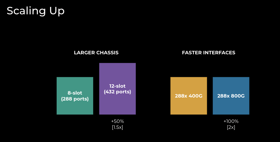 Figure 4: EBB techniques to scale up
In contrast to the dependency on vendors/industry in scaling up, scaling out (illustrated in Figure 5) is more under our control and has historically taken two flavors in EBB:
- Adding more Backbone planes. Going from four to eight planes results in doubling capacity globally; however, this technique has the following considerations:
- Implementation is quite disruptive and requires a lot of planning, specifically when it comes to fiber restriping (this needs to be coordinated in many locations simultaneously)
- Higher power and space requirements globally, but power density per rack remains the same
- Routing support for planes with uneven capacity can be complex
- Additional capacity on interconnects might be needed for compatibility with the final Backbone design
- Doesn’t require introducing new technology
- We can add multiple devices per plane. This technique is more sophisticated and allows us to scale capacity only in a chosen location. Considerations include:
- Implementation is quite disruptive for the target site and requires a moderate amount of planning to execute
- Higher power and space requirements in the target location, but power density per rack remains the same
- Interconnect with other layers might be more challenging: full mesh needs to be extended to Nx devices
- Introduces new failure modes: Device failure can impact some but not all of the of the Backbone in that plane/site
- Network operations can become more complex due to new failure modes and the handling of sets of devices (software upgrades, maintenance, etc.)
- Doesn’t require introducing new technology
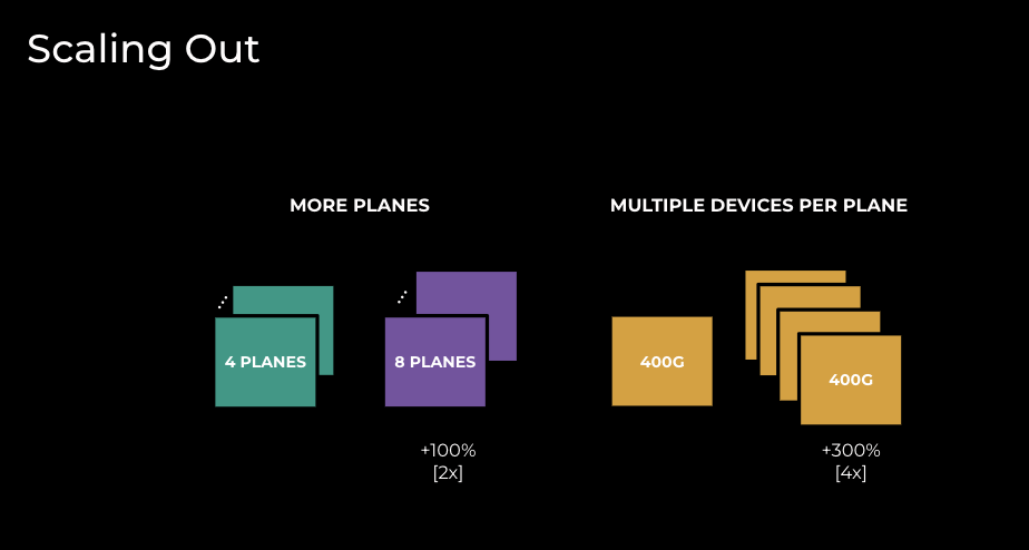 Figure 5: EBB techniques to scale out
Scaling up and scaling out are not mutually exclusive, and in our 10X Backbone journey we have used them both.
IP and Optical Integration
The third technique to scale to 10X Backbone is IP and optical integration. By leveraging ZR technology, we are changing the power footprint per terabit in the network.
Prior to ZR:
- We had many transponders per router. Each of the transponders consumed up to 2kW for 4.8-6.4Tb of capacity.
- There was a clear demarcation between IP and optical layers. This permitted work to occur at either layer with simple coordination.
With ZR:
- We no longer need transponders; this functionality is now in the plugs in the router. By removing transponders, we recover large amounts of space and power.
- Each of the plugs consumes 10-15W of incremental power.
- As a result of ZR plugs being installed in the routers, the split between IP and optical functions is not as clear as before.
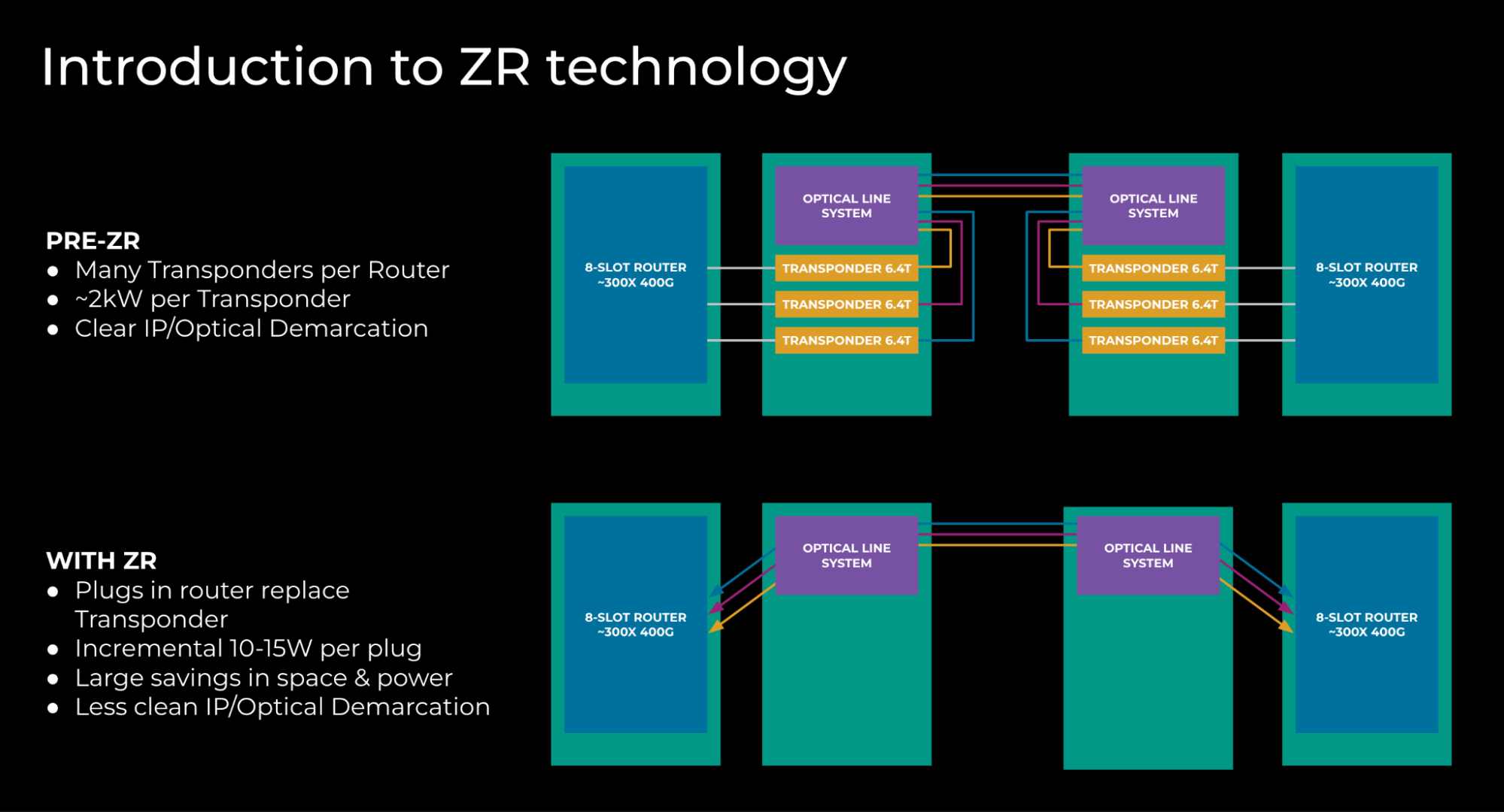 Figure 6: Network topology before and after ZR introduction
In summary, the use of ZR transceivers increases the power consumption in the router, which is offset by the considerable power savings from removing standalone transponders. In aggregate, we use 80 to 90% less power.
Using ZR technology has introduced important high-level changes:
- Cost and power efficiency:
- The same Backbone capacity can be deployed in a smaller S&P envelope
- Rack allocation between optical and IP devices goes from 90/10 (prior to ZR) to 60/40 (with ZR)
- Prior to ZR, we could land 1x fiber pairs/rack; with ZR, since we don’t use standalone transponders, we can land 4x fiber pairs/rack
- Simplifies network deployments; installing a set of pluggables instead of standalone transponders makes network deployments easier and more predictable
- Uses fewer active devices and therefore simplifies network operations
- Enables interoperability and vendor diversity
- Optical channel terminates in IP devices, and the demarcation of optical and IP is more complex than in non-ZR scenarios
- Telemetry and collections on the state of the optical channel is bound to IP devices, causing additional CPU consumption
By leveraging DC metro architecture, IP platform scaling, and IP/Optical integration, we transformed EBB from the experimental network of 2016 to a large-scale Backbone that supports all DC<>DC traffic at Meta.
AI Backbone
Over the last 18 months, we’ve seen an increasing interest in growing the megawatts footprint in support of building larger GPU clusters. The requirements have grown beyond what can fit in an existing data center campus, even considering undeveloped land or land adjacent to existing locations. Right now cluster performance is impacted by latency between endpoints, so we began to search for suitable expansion locations within bounded geographical proximity, expanding outwards until we achieve the target scale for a region.
As we identify sites of interest, we work with our fiber-sourcing team to determine the timing and feasibility to connect to existing locations at a very high scale as well as the most appropriate technology to utilize. In most cases, construction work is needed to place additional fiber in the ground, due to the significant quantities required.
We came up with three solutions based on the necessary reach:
- FR plugs: A solution that addresses buildings in the 3-kilometer range. (Note: We make some different assumptions about loss/connector count to permit this distance versus the standard specification, which states 2 kilometers.)
- LR plugs: Increasing the distance to a 10-kilometer range by using longer reach optics.
- ZR plugs + Optical DWDM (dense wavelength division multiplexing) technology: To go beyond 10-kilometer range, we need active optical components to multiplex and amplify the signals to get the desired reach. Multiplexing reduces the fiber count by a factor of 64 versus FR/LR.
For longer reach connectivity, a more complex solution is required. We use a relatively tried-and-tested design incorporating optical-protection switching, albeit using the latest generation C+L-Band 800G ZR technology.
Today’s requirements are at the lower end of the distance capabilities, and the initial deployments do not require any of the intermediate amplification sites that come into play when you go beyond 150 kilometers. This is fortunate, as these sites would be quite large given the amount of fiber pairs to be amplified (meaning additional lead times for construction, planning permits,etc.).
Protection switching introduces some additional operational challenges to how we run the network, as we require external tooling/monitoring to determine if the underlying connectivity for an IP circuit is in a protected or unprotected state. The primary reason to use them is to reduce the number of ports that we consume on the IP platforms, versus providing protection at the IP layer with additional capacity.
With this design, each fiber pair can carry 64x 800G (51.2T). To achieve the overall capacity needed between a given site-pair, we just scale this horizontally.
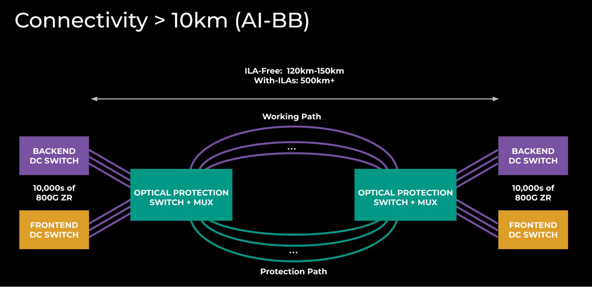
Figure 7: AI Backbone topology
The above diagram underscores the scale of these interconnects. Right now, a single AI Backbone site-pair is twice the size of the global backbone that we’ve been building for the last 10 years.
This presents many interesting challenges in how we deploy and provision this capacity. We’ll be putting a lot of time and effort into streamlining the sheer volume of this equipment and these connections as we complete the physical build-out of the fiber.
What We Learned and What the Future Holds
Scaling EBB has been a wild journey over the last eight or nine years, and it is a story of unexpected acceleration, where our scalability plans had to be accelerated, from 2028 to 2024.
These are our key learnings:
- 10x Backbone is possible because of the innovation in scaling up and scaling out.
- Pre-building scalable metro designs enables a faster response to network growth.
- IP/optical integration reduces the number of active devices, space and power footprint, and allows further scaling.
- Re-using 10X Backbone technology enables the build of AI Backbone.
Meta is planning to build city-size DCs, and our Backbone has to evolve and scale.
- We see leaf-and-spine architecture as the next step to scale out our platforms. This architecture provides the needed scale with fewer disruptive scaling steps.
- We will execute on the initial plan for AI Backbone, iterate as we go to more sites, and mature our operations. Throughout this process, we’ll come to understand AI intricacies as they develop through our optical network.
The post 10X Backbone: How Meta Is Scaling Backbone Connectivity for AI appeared first on Engineering at Meta.
]]>The post Design for Sustainability: New Design Principles for Reducing IT Hardware Emissions appeared first on Engineering at Meta.
]]>The data centers, server hardware, and global network infrastructure that underpin Meta’s operations are a critical focus to address the environmental impact of our operations. As we develop and deploy the compute capacity and storage racks used in data centers, we are focused on our goal to reach net zero emissions across our value chain in 2030. To do this, we prioritize interventions to reduce emissions associated with this hardware, including collaborating with hardware suppliers to reduce upstream emissions.
What Is Design for Sustainability?
Design for Sustainability is a set of guidelines, developed and proposed by Meta, to aid hardware designers in reducing the environmental impact of IT racks. This considers various factors such as energy efficiency and the selection, reduction, circularity, and end-of-life disposal of materials used in hardware. Sustainable hardware design requires collaboration between hardware designers, engineers, and sustainability experts to create hardware that meets performance requirements while limiting environmental impact.
In this guide, we specifically focus on the design of racks that power our data centers and offer alternatives for various components (e.g., mechanicals, cooling, compute, storage and cabling) that can help rack designers make sustainable choices early in the product’s lifecycle.
Our Focus on Scope 3 Emissions
To reach our net zero goal, we are primarily focused on reducing our Scope 3 (or value chain) emissions from physical sources like data center construction and our IT hardware (compute, storage and cooling equipment) and network fiber infrastructure.
While the energy efficiency of the hardware itself deployed in our data centers helps reduce energy consumption, we have to also consider IT hardware emissions associated with the manufacturing and delivery of equipment to Meta, as well as the end-of-life disposal, recycling, or resale of this hardware.
Our methods for controlling and reducing Scope 3 emissions generally involve optimizing material selection, choosing and developing lower carbon alternatives in design, and helping to reduce the upstream emissions of our suppliers.
For internal teams focused on hardware, this involves:
- Optimizing hardware design for the lowest possible emissions, extending the useful life of materials as much as possible with each system design, or using lower carbon materials.
- Being more efficient by extending the useful life of IT racks to potentially skip new generations of equipment.
- Harvesting server components that are no longer available to be used as spares. When racks reach their end-of-life, some of the components still have service life left in them and can be harvested and reused in a variety of ways. Circularity programs harvest components such as dual In-line memory modules (DIMMs) from end-of-life racks and redeploy them in new builds.
- Knowing the emissions profiles of suppliers, components, and system designs. This in turn informs future roadmaps that will further reduce emissions.
- Collaborating with suppliers to electrify their manufacturing processes, to transition to renewable energy, and to leverage lower carbon materials and designs.
These actions to reduce Scope 3 emissions from our IT hardware also have the additional benefit of reducing the amount of electronic waste (e-waste) generated from our data centers.
An Overview of the Types of Racks We Deploy
There are many different rack designs deployed within Meta’s data centers to support different workloads and infrastructure needs, mainly:
- AI – AI training and inference workloads
- Compute – General compute needed for running Meta’s products and services
- Storage – Storing and maintaining data used by our products
- Network – Providing Low-latency interconnections between servers
While there are differences in architecture across these different rack types, most of these racks apply general hardware design principles and contain active and passive components from a similar group of suppliers. As such, the same design principles for sustainability apply across these varied rack types.
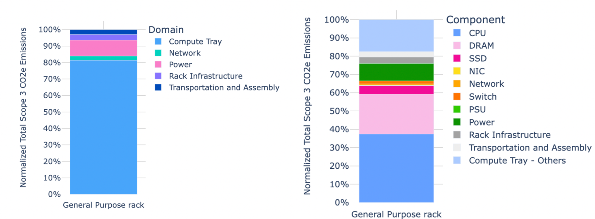
Within each rack, there are five main categories of components that are targeted for emissions reductions:
- Compute (i.e., memory, HDD/SSD)
- Storage
- Network
- Power
- Rack infrastructure (i.e., mechanical and thermals)
The emissions breakdown for a generic compute rack is shown below.
Our Techniques for Reducing Emissions
We focus on four main categories to address emissions associated with these hardware components:
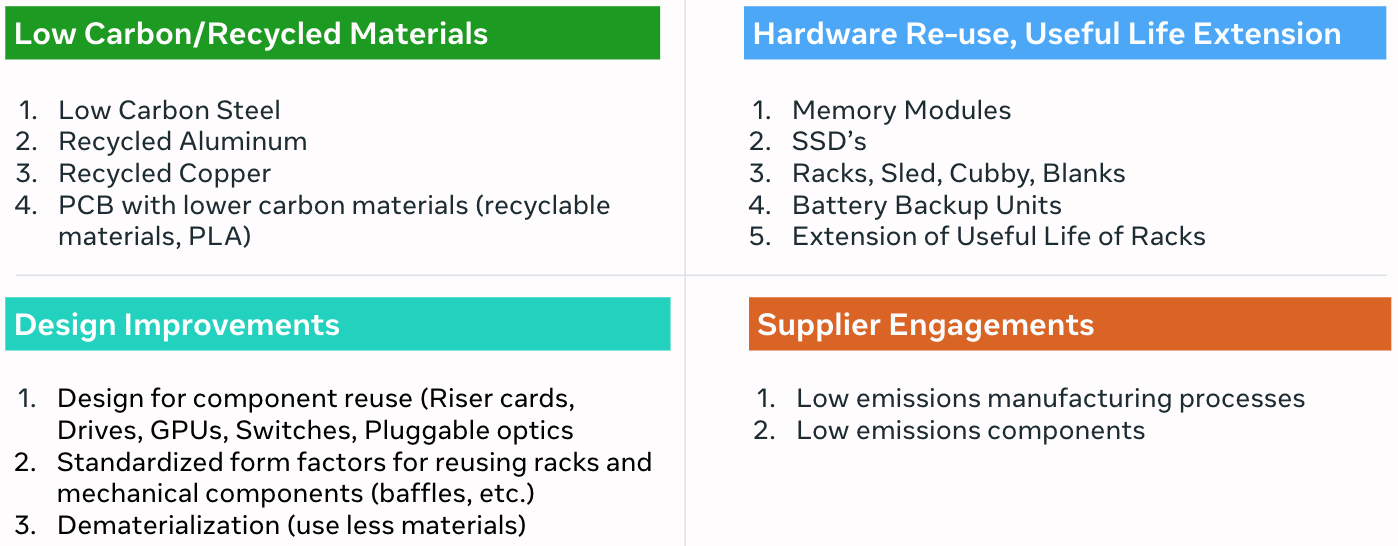
We will cover a few of the levers listed above in detail below.
Modular Rack Designs
Modular Design which allows older rack components to be re-used in newer racks. Open Rack designs (ORv2 & ORv3) form the bulk of high volume racks that exist in our data centers.

Here are some key aspects of the ORv3 modular rack design:
- ORv3 separates Power Supply Units (PSUs) and Battery Backup Units (BBUs) into their own shelves.
This allows for more reliable and flexible configurations, making repairs and replacements easier as each field replaceable unit (FRU) is toolless to replace. - Power and flexibility
The ORv3 design includes a 48 V power output, which allows the power shelf to be placed anywhere in the rack. This is an improvement over the previous ORV2 design, which limited the power shelf to a specific power zone - Configurations
The rack can accommodate different configurations of PSU and BBU shelves to meet various platform and regional requirements. For example, North America uses a dual AC input per PSU shelf, while Europe and Asia use a single AC input. - Commonization effort
There is an ongoing effort to design a “commonized” ORv3 rack frame that incorporates features from various rack variations into one standard frame. This aims to streamline the assembly process, reduce quality risks, and lower overall product costs - ORv3N
A derivative of ORv3, known as ORv3N, is designed for network-specific applications. It includes in-rack PSU and BBU, offering efficiency and cost improvements over traditional in-row UPS systems
These design principles should continue to be followed in successive generations of racks. With the expansion of AI workloads, new specialized racks for compute, storage, power and cooling are being developed that are challenging designers to adopt the most modular design principles.
Re-Using/Retrofitting Existing Rack Designs
Retrofitting existing rack designs for new uses/high density is a cost-effective and sustainable approach to meet evolving data center needs. This strategy can help reduce e-waste, lower costs, and accelerate deployment times. Benefits of re-use/retrofitting include:
- Cost savings
Retrofitting existing racks can be significantly cheaper compared to purchasing new racks. - Reduced e-waste
Reusing existing racks reduces the amount of e-waste generated by data centers. - Faster deployment
Retrofitting existing racks can be completed faster than deploying new racks, as it eliminates the need for procurement and manufacturing lead times. - Environmental benefits
Reducing e-waste and reusing existing materials helps minimize the environmental impact of data centers.
There are several challenges when considering re-using or retrofitting racks:
- Compatibility issues
Ensuring compatibility between old and new components can be challenging. - Power and cooling requirements
Retrofitting existing racks may require upgrades to power and cooling systems to support new equipment. - Scalability and flexibility
Retrofitting existing racks may limit scalability and flexibility in terms of future upgrades or changes. - Testing and validation
Thorough testing and validation are required to ensure that retrofitted racks meet performance and reliability standards.
Overall, the benefits of retrofitting existing racks are substantial and should be examined in every new rack design.
Green Steel
Steel is a significant portion of a rack and chassis and substituting traditional steel with green steel can reduce emissions. Green steel is typically produced using electric arc furnaces (EAF) instead of traditional basic oxygen furnaces (BOF), allowing for the use of clean and renewable electricity and a higher quantity of recycled content. This approach significantly reduces carbon emissions associated with steel production. Meta collaborates with suppliers who offer green steel produced with 100% clean and renewable energy.
Recycled Steel, Aluminum, and Copper
While steel is a significant component of rack and chassis, aluminum and copper are extensively used in heat sinks and wiring. Recycling steel, aluminum, and copper saves significant energy needed to produce hardware from raw materials.
As part of our commitment to sustainability, we now require all racks/chassis to contain a minimum of 20% recycled steel. Additionally, all heat sinks must be manufactured entirely from recycled aluminum or copper. These mandates are an important step in our ongoing sustainability journey.
Several of our steel suppliers, such as Tata Steel, provide recycled steel. Product design teams may ask their original design manufacturer (ODM) partners to make sure that recycled steel is included in the steel vendor(s) selected by Meta’s ODM partners. Similarly, there are many vendors that are providing recycled aluminum and copper products.
Improving Reliability to Extend Useful Life
Extending the useful life of racks, servers, memory, and SSDs helps Meta reduce the number of hardware equipment that needs to be ordered. This has helped achieve significant reductions in both emissions and costs.
A key requirement for extending useful life of hardware is the reliability of the hardware component or rack. Benchmarking reliability is an important element to determine whether hardware life extensions are feasible and for how long. Additional consideration needs to be given to the fact that spares and vendor support may have diminishing availability. Also, extending hardware life also comes with the risk of increased equipment failure, so a clear strategy to deal with the higher incidence of potential failure should be put in place.
Dematerialization
Dematerialization and removal of unnecessary hardware components can lead to a significant reduction in the use of raw materials, water, and/or energy. This entails reducing the use of raw materials such as steel on racks or removing unnecessary components on server motherboards while maintaining the design constraints established for the rack and its components.
Dematerialization also involves consolidating multiple racks into fewer, more efficient ones, reducing their overall physical footprint.
Extra components on hardware boards are included for several reasons:
- Future-proofing
Components might be added to a circuit board in anticipation of future upgrades or changes in the design. This allows manufacturers to easily modify the board without having to redesign it from scratch. - Flexibility
Extra components can provide flexibility in terms of configuration options. For example, a board might have multiple connectors or interfaces that can be used depending on the specific application. - Debugging and testing
Additional components can be used for debugging and testing purposes. These components might include test points, debug headers, or other features that help engineers diagnose issues during development. - Redundancy
In some cases, extra components are included to provide redundancy in case one component fails. This is particularly important in high-reliability applications where system failure could have significant consequences. - Modularity
Extra components can make a board more modular, allowing users to customize or upgrade their system by adding or removing modules. - Regulatory compliance
Some components might be required for regulatory compliance, such as safety features or electromagnetic interference (EMI) filtering.
In addition, changes in requirements over time can also lead to extra components. While it is very difficult to modify systems in production, it is important to make sure that each hardware design optimizes for components that will be populated.
Examples of extra components on hardware boards include:
- Unpopulated integrated circuit (IC) sockets or footprints
- Unused connectors or headers
- Test points or debug headers
- Redundant power supplies or capacitors
- Optional memory or storage components
- Unconnected or reserved pins on ICs
In addition to hardware boards, excess components may also be present in other parts of the rack. Removing excess components can lead to lowering the emissions footprint of a circuit board or rack.
Productionizing New Technologies With Lower Emissions
Productionizing new technologies can help Meta significantly reduce emissions. Memory and SSD/HDD are typically the single largest source of embodied carbon emissions in a server rack. New technologies can help Meta reduce emissions and costs while providing a substantially higher power-normalized performance.
Examples of such technologies include:
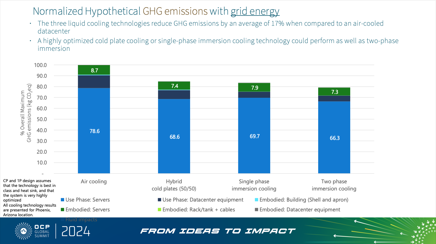
- Transitioning to SSD from HDD can reduce emissions by requiring fewer drives, servers, racks, BBUs, and PSUs, as well as help reduce overall energy usage.
- Depending on local environmental conditions, and the data center’s workload, using liquid cooling in server racks can be up to 17% more carbon-efficient than traditional air cooling.
Teams can explore additional approaches to reduce emissions associated with memory/SSD/HDD which include:
- Alternate technologies such as phase-change memory (PCM) or Magnetoresistive Random-Access Memory (MRAM) that have the same performance with low carbon.
- Use Low-Power Double Data Rates (LPDDRs ) for low power consumption and high bandwidth instead of DDR.
- Removing/reusing unused memory modules to reduce energy usage or down-clocking them during idle periods.
- Using fewer high capacity memory modules to reduce power and cooling needs. Use High Bandwidth Memory (HBM) which uses much less energy than the DDR memory.
Choosing the Right Suppliers
Meta engages with suppliers to reduce emissions through its net zero supplier engagement program. This program is designed to set GHG reduction targets with selected suppliers to help achieve our net zero target. Key aspects of the program include:
- Providing capacity building: Training suppliers on how to measure emissions, set science-aligned targets, build reduction roadmaps, procure renewable energy, and understand energy markets.
- Scaling up: In 2021 the program started with 39 key suppliers; by 2024 it expanded to include 183 suppliers, who together account for over half of Meta’s supplier-related emissions.
- Setting target goals: Meta aims to have two-thirds of its suppliers set science-aligned greenhouse gas reduction targets by 2026 . As of end-2024, 48% (by emissions contribution) have done so.
The Clean Energy Procurement Academy (CEPA), launched in 2023 (with Meta and other corporations), helps suppliers — especially in the Asia-Pacific region — learn how to procure renewable energy via region-specific curricula.
The Road to Net Zero Emissions
The Design for Sustainability principles outlined in this guide represent an important step forward in Meta’s goal to achieve net zero emissions in 2030. By integrating innovative design strategies such as modularity, reuse, retrofitting, and dematerialization, alongside the adoption of greener materials and extended hardware lifecycles, Meta can significantly reduce the carbon footprint of its data center infrastructure. These approaches not only lower emissions but also drive cost savings, e-waste reductions, and operational efficiency, reinforcing sustainability as a core business value.
Collaboration across hardware designers, engineers, suppliers, and sustainability experts is essential to realize these goals. The ongoing engagement with suppliers further amplifies the impact by addressing emissions across our entire value chain. As Meta continues to evolve its rack designs and operational frameworks, the focus on sustainability will remain paramount, ensuring that future infrastructure innovations support both environmental responsibility and business performance.
Ultimately, the success of these efforts will be measured by tangible emissions reductions, extended useful life of server hardware, and the widespread adoption of low carbon technologies and materials.
The post Design for Sustainability: New Design Principles for Reducing IT Hardware Emissions appeared first on Engineering at Meta.
]]>The post How Meta Is Leveraging AI To Improve the Quality of Scope 3 Emission Estimates for IT Hardware appeared first on Engineering at Meta.
]]>As Meta focuses on achieving net zero emissions in 2030, understanding the carbon footprint of server hardware is crucial for making informed decisions about sustainable sourcing and design. However, calculating the precise carbon footprint is challenging due to complex supply chains and limited data from suppliers. IT hardware used in our data centers is a significant source of emissions, and the embodied carbon associated with the manufacturing and transportation of this hardware is particularly challenging to quantify.
To address this, we developed a methodology to estimate and track the carbon emissions of hundreds of millions of components in our data centers. This approach involves a combination of cost-based estimates, modeled estimates, and component-specific product carbon footprints (PCFs) to provide a detailed understanding of embodied carbon emissions. These component-level estimates are ranked by the quality of data and aggregated at the server rack level.
By using this approach, we can analyze emissions at multiple levels of granularity, from individual screws to entire rack assemblies. This comprehensive framework allows us to identify high-impact areas for emissions reduction.
Our ultimate goal is to drive the industry to adopt more sustainable manufacturing practices and produce components with reduced emissions. This initiative underscores the importance of high-quality data and collaboration with suppliers to enhance the accuracy of carbon footprint calculations to drive more sustainable practices.
We leveraged AI to help us improve this database and understand our Scope 3 emissions associated with IT hardware by:
- Identifying similar components and applying existing PCFs to similar components that lack these carbon estimates.
- Extracting data from heterogeneous data sources to be used in parameterized models.
- Understanding the carbon footprint of IT racks and applying generative AI (GenAI) as a categorization algorithm to create a new and standard taxonomy. This taxonomy helps us understand the hierarchy and hotspots in our fleet and allows us to provide insights to the data center design team in their language. We hope to iterate on this taxonomy with the data center industry and agree on an industry-wide standard that allows us to compare IT hardware carbon footprints for different types and generations of hardware.
Why We Are Leveraging AI
For this work we used various AI methods to enhance the accuracy and coverage of Scope 3 emission estimates for our IT hardware. Our approach leverages the unique strengths of both natural language processing (NLP) and large language models (LLMs).
NLP For Identifying Similar Components
In our first use case (Identifying similar components with AI), we employed various NLP techniques such as Term Frequency-Inverse Document Frequency (TF-IDF) and Cosine similarity to identify patterns within a bounded, relatively small dataset. Specifically, we applied this method to determine the similarity between different components. This approach allowed us to develop a highly specialized model for this specific task.
LLMs For Handling and Understanding Data
LLMs are pre-trained on a large corpus of text data, enabling them to learn general patterns and relationships in language. They go through a post-training phase to adapt to specific use cases such as chatbots. We apply LLMs, specifically Llama 3.1, in the following three different scenarios:
- To extract and process information from diverse data sources. The benefit of LLMs is that the model can recognize different representations of the same information, even if formatted or phrased differently. (see section: Extracting Data From Heterogeneous Data)
- To understand potential groupings of components, aiding in the creation of a new taxonomy. (see section: A Component-Level Breakdown of IT Hardware Emissions Using AI)
- Once categories are identified, we use an LLM to strictly classify components based on text strings. This method allows us to save significant training time compared to a traditional AI model, as LLMs can be quickly prompt-engineered to handle various tasks. (see section: A Component-Level Breakdown of IT Hardware Emissions Using AI)
Unlike the first use case, where we needed a highly specialized model to detect similarities, we opted for LLM for these three use cases because it leverages general human language rules. This includes handling different units for parameters, grouping synonyms into categories, and recognizing varied phrasing or terminology that conveys the same concept. This approach allows us to efficiently handle variability and complexity in language, which would have required significantly more time and effort to achieve using only traditional AI.
Identifying Similar Components With AI
When analyzing inventory components, it’s common for multiple identifiers to represent the same parts or slight variations of them. This can occur due to differences in lifecycle stages, minor compositional variations, or new iterations of the part.
PCFs following the GHG Protocol are the highest quality input data we can reference for each component, as they typically account for the Scope 3 emissions estimates throughout the entire lifecycle of the component. However, conducting a PCF is a time-consuming process that typically takes months. Therefore, when we receive PCF information, it is crucial to ensure that we map all the components correctly.
PCFs are typically tied to a specific identifier, along with aggregated components. For instance, a PCF might be performed specifically for a particular board in a server, but there could be numerous variations of this specific component within an inventory. The complexity increases as the subcomponents of these items are often identical, meaning the potential impact of a PCF can be significantly multiplied across a fleet.
To maximize the utility of a PCF, it is essential to not only identify the primary component and its related subcomponents but also identify all similar parts that a PCF could be applied to. If these similar components are not identified their carbon footprint estimates will remain at a lower data quality. Therefore, identifying similar components is crucial to ensure that we:
- Leverage PCF information to ensure the highest data quality for all components.
- Maintain consistency within the dataset, ensuring that similar components have the same or closely aligned estimates.
- Improve traceability of each component’s carbon footprint estimate for reporting.
To achieve this, we employed a natural language processing (NLP) algorithm, specifically tailored to the language of this dataset, to identify possible proxy components by analyzing textual descriptions and filtering results by component category to ensure relevance.
The algorithm identifies proxy components in two distinct ways:
- Leveraging New PCFs: When a new PCF is received, the algorithm uses it as a reference point. It analyzes the description names of components within the same category to identify those with a high percentage of similarity. These similar components can be mapped to a representative proxy PCF, allowing us to use high-quality PCF data in similar components.
- Improving Low Data Quality Components: For components with low data quality scores, the algorithm operates in reverse with additional constraints. Starting with a list of low-data-quality components, the algorithm searches for estimates that have a data quality score greater than a certain threshold. These high-quality references can then be used to improve the data quality of the original low-scoring components.
Meta’s Net Zero team reviews the proposed proxies and validates our ability to apply them in our estimates. This approach enhances the accuracy and consistency of component data, ensures that high-quality PCF data is effectively utilized across similar components, and enables us to design our systems to more effectively reduce emissions associated with server hardware.
Extracting Data From Heterogeneous Data Sources
When PCFs are not available, we aim to avoid using spend-to-carbon methods because they tie sustainability too closely to spending on hardware and can be less accurate due to the influence of factors like supply chain disruptions.
Instead, we have developed a portfolio of methods to estimate the carbon footprint of these components, including through parameterized modeling. To adapt any model at scale, we require two essential elements: a deterministic model to scale the emissions, and a list of data input parameters. For example, we can scale the carbon footprint calculation for a component by knowing its constituent components’ carbon footprint.
However, applying this methodology can be challenging due to inconsistent description data or locations where information is presented. For instance, information about cables may be stored in different tables, formats, or units, so we may be unable to apply models to some components due to difficulty in locating input data.
To overcome this challenge, we have utilized large language models (LLMs) that extract information from heterogeneous sources and inject the extracted information into the parameterized model. This differs from how we apply NLP, as it focuses on extracting information from specific components. Scaling a common model ensures that the estimates provided for these parts are consistent with similar parts from the same family and can inform estimates for missing or misaligned parts.
We applied this approach to two specific categories: memory and cables. The LLM extracts relevant data (e.g., the capacity for memory estimates and length/type of cable for physics-based estimates) and scales the components’ emissions calculations according to the provided formulas.
A Component-Level Breakdown of IT Hardware Emissions Using AI
We utilize our centralized component carbon footprint database not only for reporting emissions, but also to drive our ability to efficiently deploy emissions reduction interventions. Conducting a granular analysis of component-level emissions enables us to pinpoint specific areas for improvement and prioritize our efforts to achieve net zero emissions. For instance, if a particular component is found to have a disproportionately high carbon footprint, we can explore alternative materials or manufacturing processes to mitigate its environmental impact. We may also determine that we should reuse components and extend their useful life by testing or augmenting component reliability. By leveraging data-driven insights at the component level and driving proactive design interventions to reduce component emissions, we can more effectively prioritize sustainability when designing new servers.
We leverage a bill of materials (BOM) to list all of the components in a server rack in a tree structure, with “children” component nodes listed under “parent” nodes. However, each vendor can have a different BOM structure, so two identical racks may be represented differently. This, coupled with the heterogeneity of methods to estimate emissions, makes it challenging to easily identify actions to reduce component emissions.
To address this challenge, we have used AI to categorize the descriptive data of our racks into two hierarchical levels:
- Domain-level: A high-level breakdown of a rack into main functional groupings (e.g., compute, network, power, mechanical, and storage)
- Component-level: A detailed breakdown that highlights the major components that are responsible for the bulk of Scope 3 emissions (e.g., CPU, GPU, DRAM, Flash, etc.)
We have developed two classification models: one for “domain” mapping, and another for “component” mapping. The difference between these mappings lies in the training data and the additional set of examples provided to each model. We then combine the two classifications to generate a mutually exclusive hierarchy.
During the exploration phase of the new taxonomy generation, we allowed the GenAI model to operate freely to identify potential categories for grouping. After reviewing these potential groupings with our internal hardware experts, we established a fixed list of major components. Once this list was finalized, we switched to using a strict GenAI classifier model as follows:
- For each rack, recursively identify the highest contributors, grouping smaller represented items together.
- Run a GenAI mutually exclusive classifier algorithm to group the components into the identified categories.
This methodology has been presented at the 2025 OCP regional EMEA summit with the goal to drive the industry toward a common taxonomy for carbon footprint emissions, and open source the methodology we used to create our taxonomy.
These groupings are specifically created to aid carbon footprint analysis, rather than for other purposes such as cost analysis. However, the methodology can be tailored for other purposes as necessary.
Coming Soon: Open Sourcing Our Taxonomies and Methodologies
As we work toward achieving net zero emissions across our value chain in 2030, this component-level breakdown methodology is necessary to help understand our emissions at the server component level. By using a combination of high-quality PCFs, spend-to-carbon data, and a portfolio of methods that leverage AI, we can enhance our data quality and coverage to more effectively deploy emissions reduction interventions.
Our next steps include open sourcing:
- The taxonomy and methodology for server rack emissions accounting.
- The taxonomy builder using GenAI classifiers.
- The aggregation methodology to improve facility reporting processes across the industry.
We are committed to sharing our learnings with the industry as we evolve this methodology, now as part of a collaborative effort with the OCP PCR group.
The post How Meta Is Leveraging AI To Improve the Quality of Scope 3 Emission Estimates for IT Hardware appeared first on Engineering at Meta.
]]>The post OCP Summit 2025: The Open Future of Networking Hardware for AI appeared first on Engineering at Meta.
]]>At Meta, we believe that open hardware is a catalyst for innovation — especially as data center infrastructure increasingly supports new and emerging AI technologies. Open hardware plays a crucial role in enabling disaggregation, allowing us to break down traditional data center technologies into their core components. This approach empowers us to build systems that are more flexible, scalable, and efficient.
Since co-founding the Open Compute Project (OCP) in 2011, Meta has shared data center and component designs, and open-sourced our network operating system, FBOSS, to inspire new ideas both within our own operations and across the industry. These efforts have played an important role in making Meta’s data centers sustainable and efficient. Today, through OCP, we continue to advance open network technologies for the next generation of AI applications.
We’re announcing several new milestones for our data center networking:
- The evolution of Disaggregated Scheduled Fabric (DSF) to support scale-out interconnect for large AI clusters that span entire data center buildings.
- A new Non-Scheduled Fabric (NSF) architecture based entirely on shallow-buffer, disaggregated Ethernet switches that will support our largest AI clusters like Prometheus.
- The addition of Minipack3N, based on NVIDIA’s Ethernet Spectrum-4 ASIC, to our portfolio of 51 Tbps OCP switches that use OCP’s SAI and Meta’s FBOSS software stack.
- The launch of the Ethernet for Scale-Up Networking (ESUN) initiative, where Meta has worked with other large-scale operators and leading Ethernet vendors to advance using Ethernet for scale-up networking (specifically the high-performance interconnects required for next-generation AI accelerator architectures..
Dual-Stage DSF: Scaling Scheduled Fabrics for Larger AI Clusters
At last year’s OCP Global Summit we shared Disaggregated Scheduled Fabric (DSF), a VOQ-based system powered by the open OCP-SAI standard and FBOSS. The DSF fabric supports an open and standard Ethernet-based RoCE interface to endpoints and accelerators across several xPUs and NICs, including Meta’s MTIA as well as from several vendors.
Over the last year, we have evolved DSF to a 2-stage architecture, scaling to support a non-blocking fabric that interconnects up to 18,432 XPUs. These clusters are a fundamental building block for constructing AI clusters that span regions (and even multiple regions) in order to meet the increased capacity and performance demands of Meta’s AI workloads.
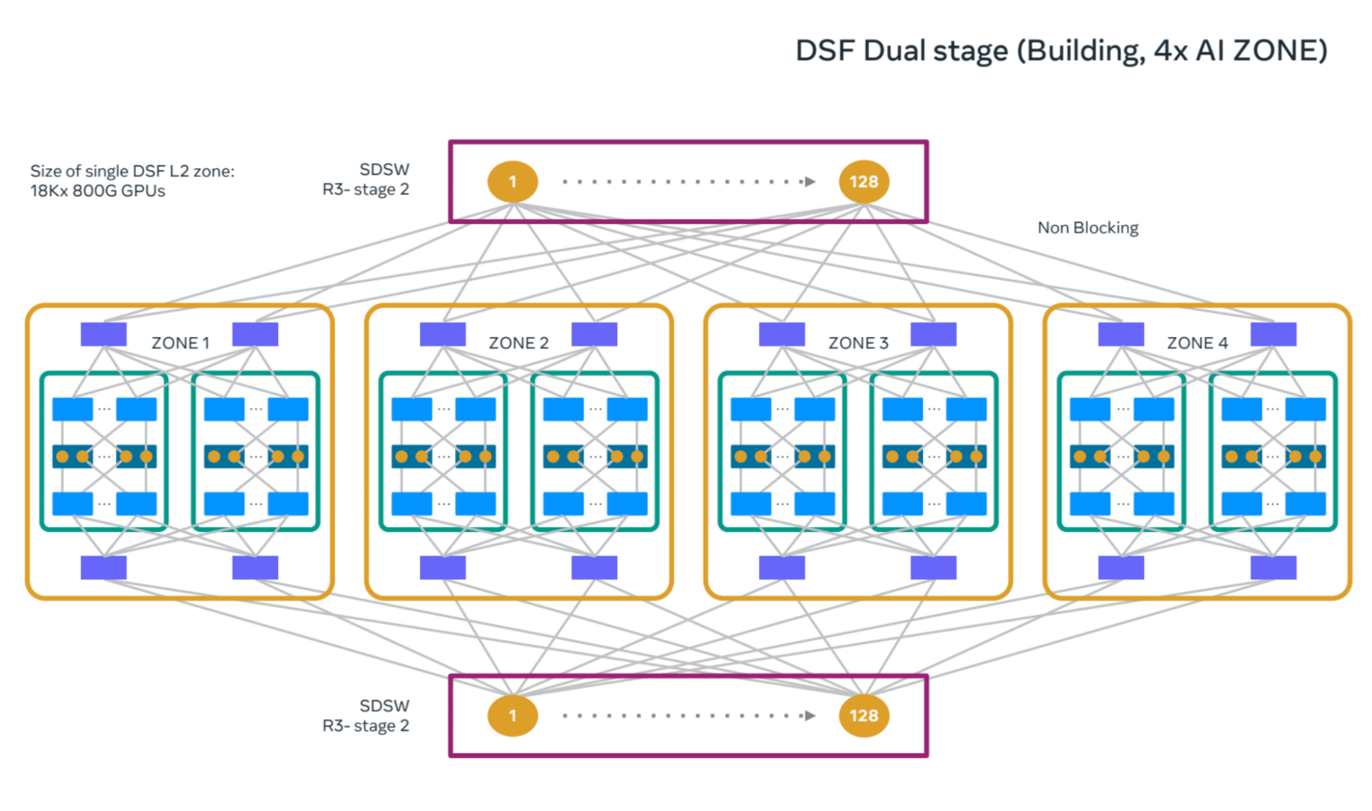
Non-Scheduled Fabrics (NSF) for Large AI Clusters
In parallel with the evolution of the DSF architecture, we have also devised a new architecture called the Non-Scheduled Fabric (NSF), with the following key features:
- Based on shallow-buffer OCP Ethernet switches.
- Delivers low round-trip latency.
- Supports adaptive routing for effective load-balancing, ensuring optimal utilization and minimizing congestion.
- Serves as foundational building block for Gigawatt-scale AI clusters like Prometheus.

New OCP Switch Platforms for Next-Generation AI Fabrics
Last year, Meta introduced two new 51T Ethernet switches: Minipack3 (based on Broadcom Tomahawk5) and Cisco 8501 (based on Cisco Silicon One G200). These OCP switches offer 51.2 Tbps (64x OSFP ports), are power-efficient without the need for retimers, and run our large-scale network operating system, FBOSS. These platforms have served as the foundation for building our next-generation frontend and backend data center fabrics.
This year, we are introducing Minipack3N, a new 51T Ethernet switch that is based on the NVIDIA Spectrum-4 switching ASIC and leverages the same system design as Minipack3.
Evolving FBOSS and SAI for DSF and NSF
![]()
Meta continues to embrace OCP-SAI as the foundation for onboarding new network fabrics, switch hardware platforms, and optical transceivers into FBOSS. Through close collaboration with vendors and the OCP community, we have evolved SAI to support advanced features and concepts, including DSF, NSF, and other enhanced routing schemes tailored for modern data center and AI workloads.
This open approach empowers developers and engineers worldwide to engage with cutting-edge hardware, contribute innovative software, and leverage these solutions for their own needs. By sharing advancements and fostering collaboration, we help accelerate progress across the industry, ensuring that open hardware and software remain at the heart of scalable, efficient, and future-ready data center infrastructure.
Optics: 2x400G FR4-LITE and 400G/2x400G DR4 Optics for 400G/800G Optical Interconnections
Last year, Meta introduced 2x400G FR4 BASE (3-km) optics, the primary solution supporting next-generation 51T platforms across both backend and frontend networks and DSFs. These optics have now been widely deployed throughout Meta’s data centers.
This year, we are expanding our portfolio with the launch of 2x400G FR4 LITE (500-m) optics. Developed as part of an efficiency initiative, FR4 LITE is optimized for the majority of intra–data center use cases, supporting fiber links up to 500 meters. This new variant is designed to accelerate optics cost reduction while maintaining robust performance for shorter-reach applications.
In addition, we are introducing the 400G DR4 OSFP-RHS optics — our first-generation DR4 solution for AI host-side NIC connectivity. Complementing this, the new 2x400G DR4 OSFP optics are being deployed on the switch side, providing connectivity from host to switch.
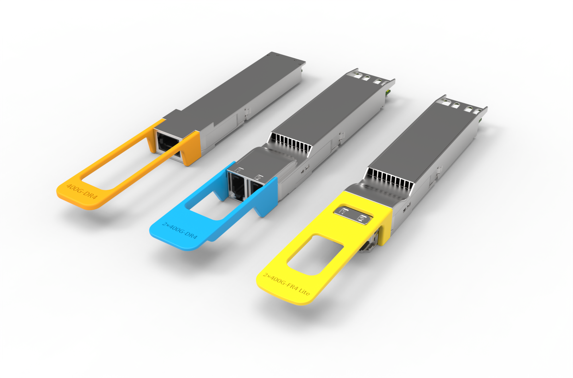
Ethernet for Scale-Up Networking in OCP: Meta’s Industry Leadership
At Meta, we recognize that the future of AI and data center infrastructure depends on open, scalable, and interoperable networking solutions. As part of our ongoing commitment to open hardware and industry collaboration, Meta is a founding participant in the new Ethernet for Scale-Up Networking (ESUN) initiative, which launched within OCP at the 2025 OCP Global Summit.
What Is ESUN?
ESUN is a new workstream within the OCP Networking Project. It functions as an open technical forum where industry operators and leading vendors can collaborate to advance the use of Ethernet technology. The specific goal of ESUN is to leverage and adapt the mature Ethernet ecosystem to meet the unique, high-performance demands of the scale-up domain within modern AI systems.
ESUN is focused specifically on the network functionality aspect of scale-up systems. The workstream is designed to address the technical challenges related to how data traffic is managed and transmitted across network switches. This includes defining best practices and standards for:
- Protocol headers
- Error handling mechanisms
- Achieving lossless data transfer across the network
The initiative brings together operators, vendors, and standards bodies to:
- Collaborate on Ethernet solutions tailored for scale-up networking.
- Focus on Ethernet framing and switching layers to ensure robust, lossless, and error-resilient multi-hop topologies.
- Align with open standards by working closely with organizations like UEC and IEEE.
Meta’s Contributions to ESUN
Meta is proud to be among the initial group of OCP members driving ESUN, alongside industry leaders that includes: AMD, Arista, ARM, Broadcom, Cisco, HPE, Marvell, Meta, Microsoft, NVIDIA, OpenAI, and Oracle.
Our contributions include:
- Technical leadership in defining the requirements for ESUN in AI clusters.
- Open collaboration with vendors and standards bodies to ensure that solutions are interoperable and not tied to proprietary technologies.
- Sharing best practices and lessons learned from deploying advanced Ethernet fabrics in Meta’s own data centers.,
An Industry Invitation: Join the Open Future
Driving progress in AI requires data center infrastructure that delivers more than just scale — it must also be flexible, efficient, and sustainable. At Meta, we envision a future where AI hardware systems are not only highly scalable, but also open and collaborative, enabling rapid innovation and adaptation to evolving workloads.
We invite engineers, developers, and industry partners to join us and the OCP community in shaping the next generation of networking hardware for AI. By working together and sharing ideas, we can accelerate the development of open, future-ready AI infrastructure that benefits the entire industry and supports the demands of tomorrow’s technologies.
The post OCP Summit 2025: The Open Future of Networking Hardware for AI appeared first on Engineering at Meta.
]]>The post Introducing the React Foundation: The New Home for React & React Native appeared first on Engineering at Meta.
]]>This incredible growth is thanks to the thousands of educators, companies, and projects that have contributed to the development of React. The community is the heart of React, and we’re proud to play a part in the cycle of open source innovation throughout the ecosystem that benefits everyone. We’re pleased to give a seat at the table to the people and companies that have made React what it is today.
Today, we are excited to announce the next step for React. Several projects within the React ecosystem, including React and React Native, as well as supporting projects such as JSX, will transition to the React Foundation. The React Foundation’s mission is to help the React community and its members. The React Foundation will maintain React’s infrastructure, organize React Conf, and create initiatives to support the React ecosystem. The React Foundation will be part of the Linux Foundation, which has long fostered a vendor-neutral environment for open source projects.
Formalizing Governance
The React Foundation’s governing board will consist of representatives from Amazon, Callstack, Expo, Meta, Microsoft, Software Mansion, and Vercel, with the intention to expand further over time.
There will be a clear separation between the business and technical governance of React. Releases, features, and technical direction will be governed by a new structure driven by the maintainers and contributors of React. This new technical governance structure will be independent of the React Foundation. The React team is actively working on this new technical governance structure and will share more details in a future post on the React blog.
Meta and the React Foundation
Meta is committing to a five-year partnership with the React Foundation, including over $3 million in funding and dedicated engineering support. This investment will ensure React’s smooth transition to independent governance while maintaining the stability and innovation the community expects. Meta will continue to invest in React and use it as our primary tool for building UI on the web and across many of Meta’s apps. Meta will also continue to have a dedicated team of engineers working full-time on React and React Native.
We believe the best of React is yet to come. The React Foundation will unlock new opportunities for collaboration, innovation, and growth that will benefit the entire ecosystem. We’re excited to see what the community will build together under this new model. With strengthened governance, broader industry participation, and continued technical excellence, React is positioned to tackle the next generation of challenges in UI development.
The post Introducing the React Foundation: The New Home for React & React Native appeared first on Engineering at Meta.
]]>The post Introducing OpenZL: An Open Source Format-Aware Compression Framework appeared first on Engineering at Meta.
]]>Today, we are excited to announce the public release of OpenZL, a new data compression framework. OpenZL offers lossless compression for structured data, with performance comparable to specialized compressors. It accomplishes this by applying a configurable sequence of transforms to the input, revealing hidden order in the data, which can then be more easily compressed. Despite applying distinct transformation permutations for every file type, all OpenZL files can be decompressed using the same universal OpenZL decompressor.
A Decade of Lessons
When Zstandard was announced, it came with a simple pitch: It promised the same or better compression ratio of prior default but at the much increased speed required by datacenter workloads. By pairing strong entropy coding with a design that fully utilized modern CPU capabilities, Zstandard offered a substantial improvement that justified its presence in datacenters.
However, while it was improved over time, remaining within the Zstandard framework offers diminishing returns. So we started looking for the next great leap in data compression.
In this quest, one pattern kept repeating: Using generic methods on structured data leaves compression gains on the table. Data isn’t just byte soup. It can be columnar, encode enums, be restricted to specific ranges, or carry highly repetitive fields. More importantly, it has predictable shapes. A bespoke compressor that leans into that structure can beat general-purpose tools on both ratio and speed. But there’s a catch — every bespoke scheme means another compressor and decompressor to create, ship, audit, patch, and trust.
OpenZL is our answer to the tension between the performance of format-specific compressors and the maintenance simplicity of a single executable binary.
Make the Structure Explicit
General compressors rely on a one-size fits all processing strategy, or alternatively spend a lot of their cycles guessing which techniques to use. OpenZL saves those cycles by making the structure an explicit input parameter. Compression can then focus on a sequence of reversible steps that surface patterns before coding.
As a user, you provide OpenZL with the data shape (via a preset or a thin format description). Then the trainer, an offline optimization component, builds an effective compression config that can be re-employed for similar data. During encoding that config resolves into a concrete decode recipe that’s embedded into the frame. The universal decoder will directly execute that recipe, without any out-of-band information.
An Example Compression Using OpenZL
As an example, let’s compress sao, which is part of the Silesia Compression Corpus. This file follows a well-defined format featuring an array of records, each one describing a star. Providing this information to OpenZL is enough to give it an edge over generic lossless compressors, which only see bytes.
Comparison on a M1 cpu, using clang-17
| Compressor | zstd -3 | xz -9 | OpenZL |
| Compressed Size | 5,531,935 B | 4,414,351 B | 3,516,649 B |
| Compression Ratio | x1.31 | x1.64 | x2.06 |
| Compression Speed | 220 MB/s | 3.5 MB/s | 340 MB/s |
| Decompression Speed | 850 MB/s | 45 MB/s | 1200 MB/s |
Crucially, OpenZL produces a higher compression ratio while preserving or even improving speed, which is critical for data center processing pipelines.
For illustration, this result is achieved using the following simple graph:
A Brief Explanation
So what is happening in this example?
We start by separating the header from the rest, a large table of structures. Then each field gets extracted into its own stream: the array of structures becomes a structure of arrays. After that point, we expect that each stream contains homogeneous data of the same type and semantic meaning. We can now focus on finding an optimal compression strategy for each one.
- SRA0 is a position on the X axis. Due to the way the table is generated, the index is mostly sorted, inviting the use of delta to reduce the range of values represented. This mechanically makes the resulting stream easier to compress.
- SDEC0 is a position on the Y axis. It’s not as well sorted as the X axis, but we can at least exploit the fact that it’s bounded between a minimum and a maximum. This makes the higher bytes more predictable, which can be exploited for better compression with the transpose operation.
- The other fields (IS, MAG, XRPM, XDPM) share a common property: their cardinality is much lower than their quantities, and there is no relation between 2 consecutive values. This makes them a good target for tokenize, which will convert the stream into a dictionary and an index list.
- The resulting dictionaries and index lists are very different. They benefit from completely different compression strategies. So they are sent to dedicated processing graphs.
The graph continues beyond these steps. But at some point, we can also stop making decisions. The main work is to group data into homogeneous streams. After that, one can count on openzl to take care of the rest.
To go even further, we would like to generate compression strategies that are specifically fine-tuned for each stream. This is where the offline trainer stage comes into play.
Generate a Compressor Automatically
It’s possible to take full control of the compression process, but it’s also not required. A faster strategy is to just describe your data and let the system learn a compression config.
Describe the input: With the Simple Data Description Language (SDDL), you sketch how the bytes map to fields — rows, columns, enums, nested records. SDDL is for parsing only; it just tells OpenZL the shape of your data. Alternatively, you can write your own parser function directly using one of the supported languages, and register it with OpenZL to delegate the logic.
Learn the config: Starting from a preset, a parser function or an SDDL description, the trainer runs a budgeted search over transform choices and parameters to produce a Plan. It can provide a full set of speed/ratio tradeoffs, or directly target the best configuration respecting some speed constraints. Internally it uses a cluster finder (to group fields that behave alike) and a graph explorer (to try candidate subgraphs and keep score).
Resolve at encode-time: While compressing, the encoder turns the Plan into a concrete recipe — the Resolved Graph. If the Plan has control points, it picks the branch that fits the data and records that choice into the frame.
Decode without coordination: Each frame chunk carries its own resolved graph. The single decoder checks it, enforces limits, and runs the steps in order. When a plan improves, you just roll out the new plan, no new decompressor needed. Old data keeps decoding; new data get improved gains.
In practice the loop is straightforward: describe (SDDL) → train (produce a plan) → compress (emit frames with resolved graphs) → decode anywhere with the same binary.
Embracing Changes: Re-Training and In-Flight Control
In the real world, data evolves constantly, in both structure and content. A compressor built for one version of a schema would have a short lifetime.
Thankfully, with the flexibility offered by compression plans, we can react swiftly to data changes. At Meta, this is the core mission of Managed Compression, originally created to automate dictionary compression with Zstandard, and presented in an earlier blog on how we improved compression at with Zstandard.
OpenZL offers a training process that updates compression plans to maintain or improve compression performance, based on provided data samples. Now the synergy with Managed Compression is apparent: Each registered use case is monitored, sampled, periodically re-trained, and receives new configs when they prove beneficial. The decompression side continues to decode both old and new data without any change.
Runtime Adaptation: A compression config can include control points that read lightweight statistics at compression time (e.g., string repetition stats, run-length, histogram skew, delta variance) and choose the best branch of the Plan to go to next. Many technologies can be used, and textbook classifiers qualify. Control points handle bursts, outliers, and seasonal shifts without brute-force exploration: exploration is bounded, in order to maintain speed expectations. Taken branches are then recorded into the frame, and the decoder just executes the recorded path.
This gives the best of both worlds: dynamic behavior at compression time to handle variations and exceptions — without turning compression into an unbounded search problem — and with zero complexity added to the decoder.
The Advantages of the Universal Decoder
OpenZL is capable of compressing a vast array of data formats, and they can all be decompressed with a single decompressor binary. Even when the compression configuration changes, the decoder does not. This may sound like operational minutiae, but it’s critical to OpenZL’s deployment success.
- One audited surface: Security and correctness reviews focus on a single binary with consistent invariants, fuzzing, and hardening; there’s no myriad of per-format tools that can drift apart.
- Fleet-wide improvements: A decoder update (security or performance — SIMD kernels, memory bounds, scheduling) benefits every compressed file, even those that predate the change.
- Operational clarity: Same binary, same CLI, same metrics and dashboards across datasets; patching and rollout are uneventful by design.
- Continuous training: With one decoder and many compression plans, we can keep improving while the system is live. Train a plan offline, try it on a small slice, then roll it out like any other config change. Backward compatibility is built-in — old frames still decode while new frames get better.
In other words, it’s possible to afford domain-specific compression without fragmenting the ecosystem.
Results With OpenZL
When OpenZL is able to understand and parse the file format, it is able to offer large improvements in compression ratio, while still providing fast compression and decompression speed. However, this is no magic bullet. When OpenZL doesn’t understand the input file format, it simply falls back to zstd.
OpenZL, through its offline training capabilities, is also able to offer a wide range of configurations in the tradeoff space of compression ratio, compression speed, and decompression speed. Unlike traditional compressors, which offer configuration by setting a compression level, OpenZL offers configuration by serializing the compressor graph. This allows an immense amount of flexibility to select diverse tradeoffs.
These results are based on datasets we’ve developed for our whitepaper. The datasets were chosen because they are highly structured and in a format that OpenZL supports. Every figure below is produced with scripts in the OpenZL repository so they can be reproduced, and the input data and logs from our runs have been uploaded to GitHub.
Note that data points connected by a line are pareto-optimal. All such points have the property that there is no point in the same dataset which beats them in both metrics.
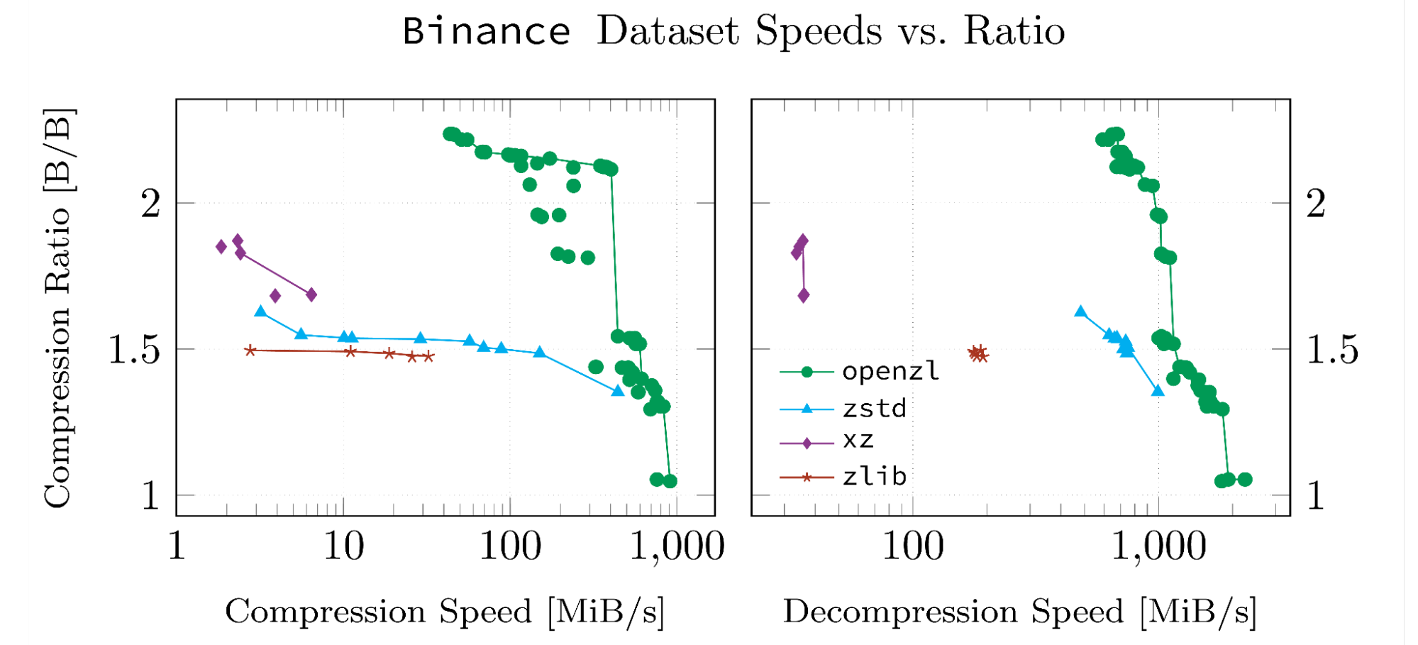
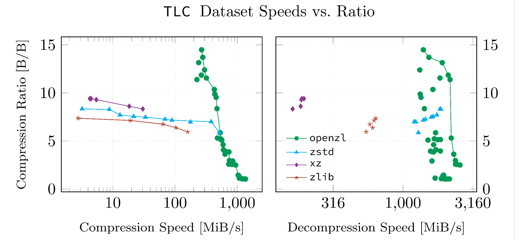

When It’s Not Useful
OpenZL relies on a description of some structure to leverage its set of transforms. When there is no structure, there is no advantage. This is typically the case in pure text documents, such as enwik or dickens. In these cases, OpenZL falls back to zstd, offering essentially the same level of performance.
Getting Started With OpenZL
OpenZL’s selection of codecs is well-suited to compressing vector, tabular, or tree-structured data, and can be expected to perform well with numeric, string, or binary data. Common examples include timeseries datasets, ML tensors, and database tables. Keep in mind that we are bound by the limits of information theory, so the input needs to have some order that can be uncovered. As time goes on, we plan to incorporate additional codecs, as described in the next section.
If your data fits one of the above categories, then give it a try! Visit the OpenZL site and our Quick Start guide to get started.
If you want to dive into the code, check out the GitHub repository for source, documentation, and examples. We welcome contributions and feedback from the community!
Where We’re Going
OpenZL’s general direction is set: make it easier to expose structures, and exploit it with automated compression plans for evolving data.
Next up: We’re extending the transform library for time-series and grid-shaped data, improving performance of codecs, and enabling the trainer to find better compression plans faster. We also are actively working to extend SDDL to describe nested data formats more flexibly. Finally, the automated compressor explorer is getting better at proposing safe, testable changes to a compression plan within a specified budget.
Where the community can help: If you have a format or a dataset with obvious structure, try compressing it with an OpenZL prebuilt Plan. If it’s promising, try generating a new plan with the trainer or customizing it with our documentation to improve it. If it’s a format that the public might want, send it to us in a PR.
You can also contribute to the OpenZL core. If you have a knack for optimizing C/C++, help us speed up the engine or add transforms to cover new data formats. If your super power is reliability, the project would surely benefit from more validation rules and resource caps. And if you care about benchmarks, add your dataset to the harness so others can reproduce your results.
How to engage: Open an issue on the GitHub issue board. If you have a use-case for which you would expect OpenZL to do better, provide a few small samples, so that we can analyze them together. You may also contribute to codec optimizations, and propose new graphs, parsers or control points. All these topics do not impact the universality of the decoder.
We believe OpenZL opens up a new universe of possibilities to the data compression field, and we’re excited to see what the open source community will do with it!
To learn more about Meta Open Source, visit our website, subscribe to our YouTube channel, or follow us on Facebook, Threads, X, Bluesky and LinkedIn.
The post Introducing OpenZL: An Open Source Format-Aware Compression Framework appeared first on Engineering at Meta.
]]>