Downloaded 588 times
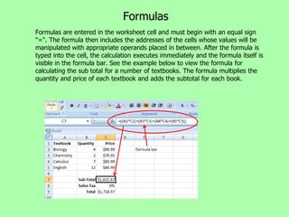
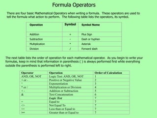
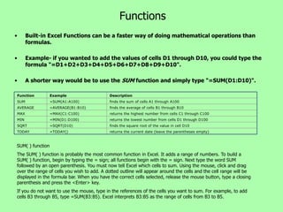

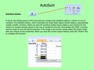
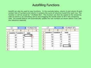
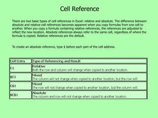
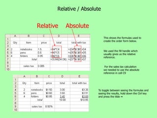

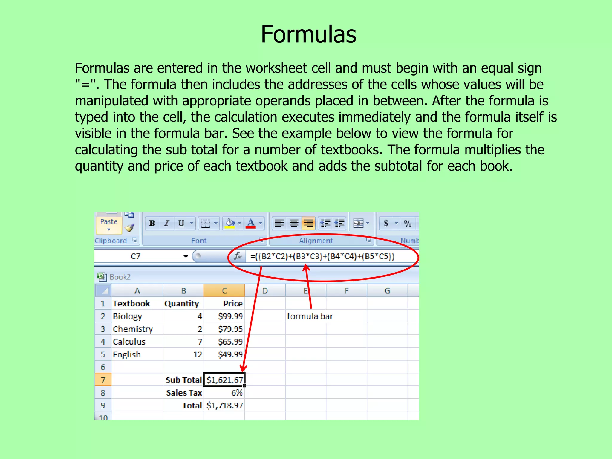
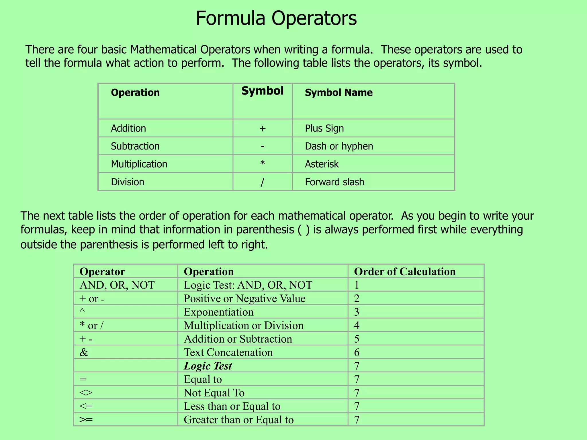
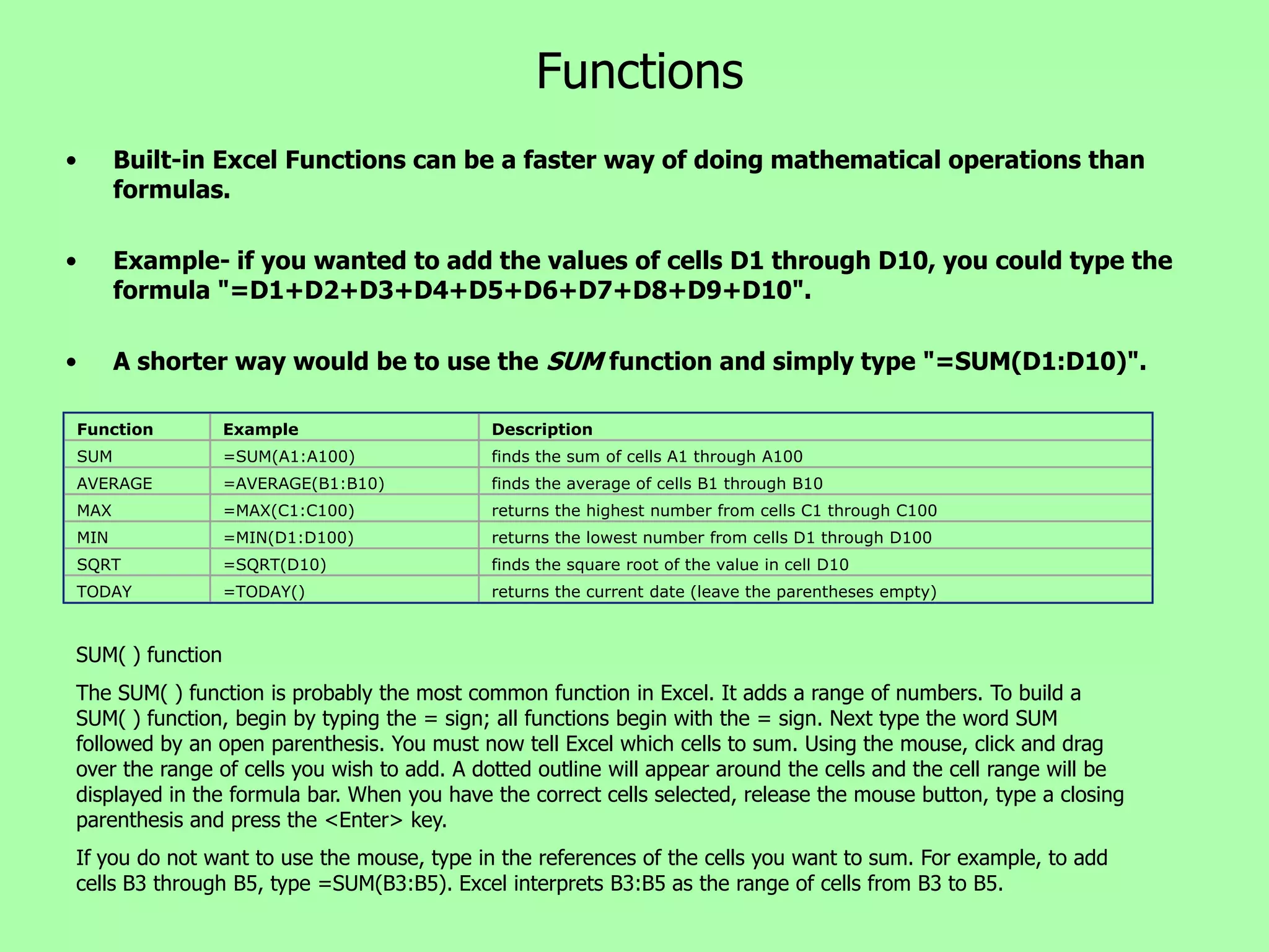
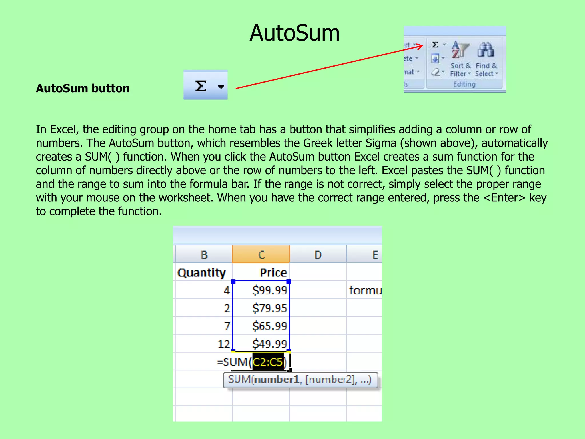

Excel allows users to enter formulas to perform calculations on worksheet data. Formulas begin with an equal sign and can reference cell addresses to manipulate cell values using mathematical operators like addition and subtraction. Common functions like SUM, AVERAGE, and MAX simplify calculations. Formulas can be copied and filled using relative or absolute cell references.


