Downloaded 37 times


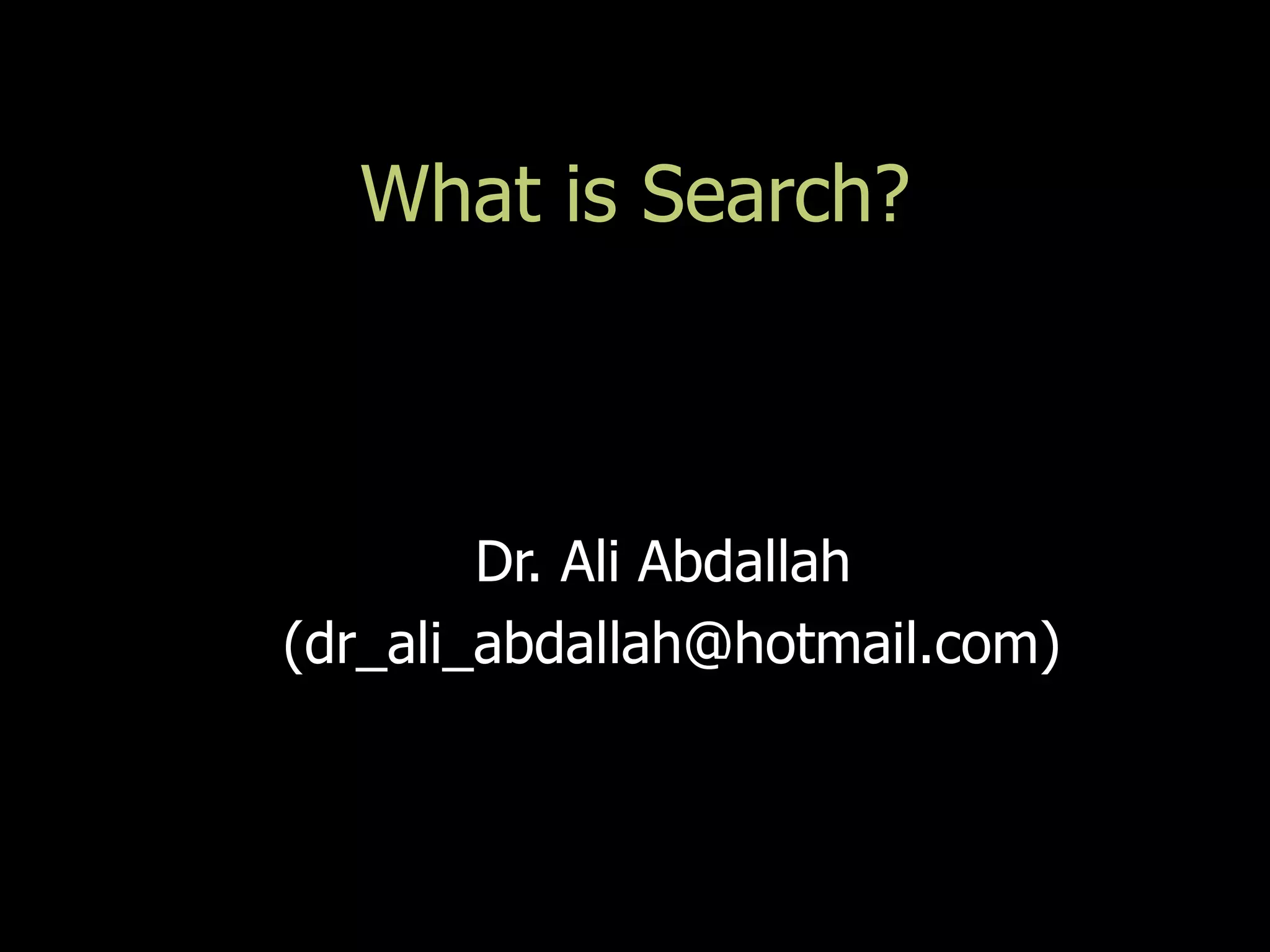
![Performance Measures
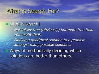
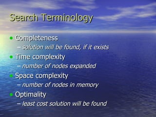
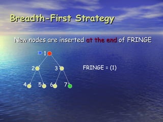
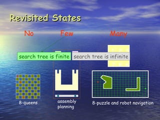
Completeness
A search algorithm is complete if it finds a
solution whenever one exists
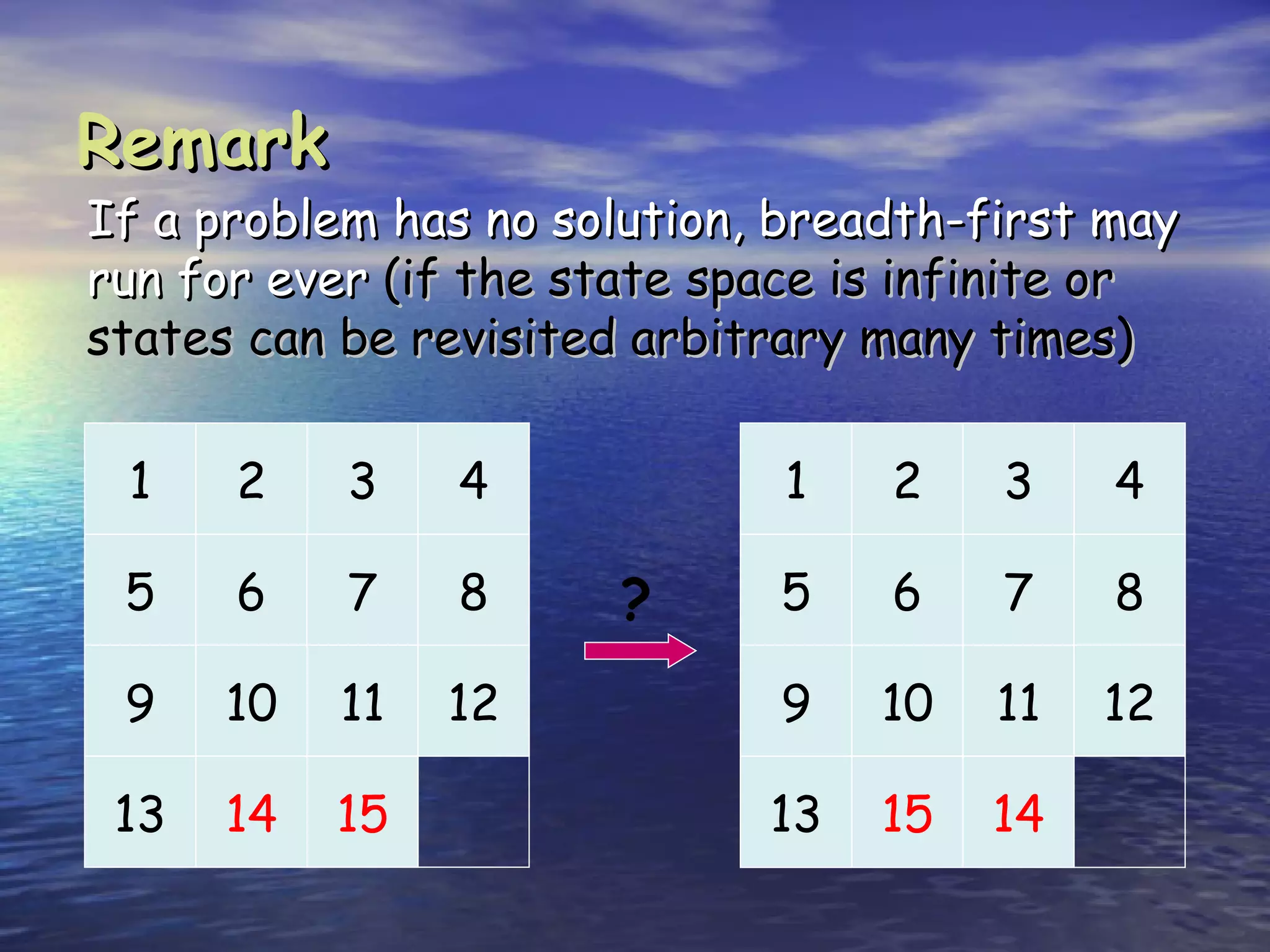
[What about the case when no solution exists?]
Optimality
A search algorithm is optimal if it returns an
optimal solution whenever a solution exists
Complexity
It measures the time and amount of memory
required by the algorithm](https://image.slidesharecdn.com/03searchblind-120428063044-phpapp02/85/03-search-blind-21-320.jpg)


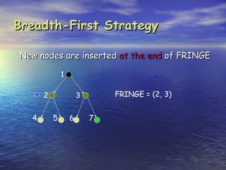
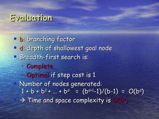


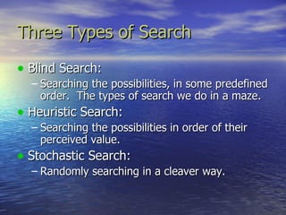
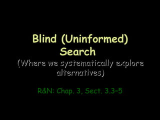
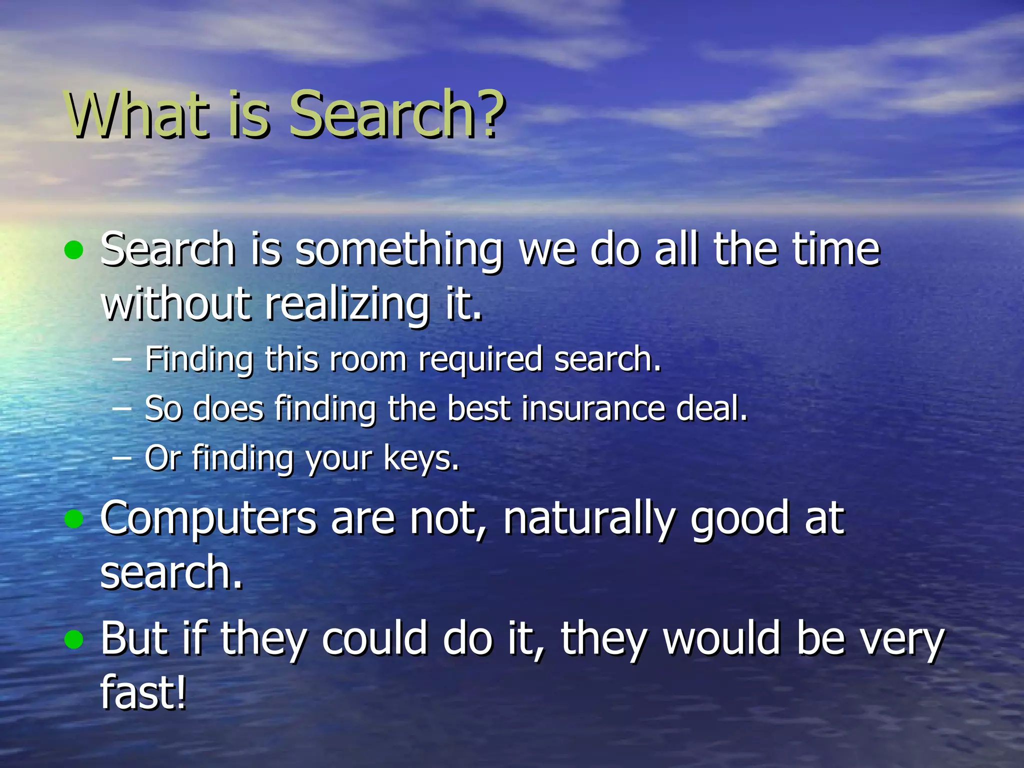
![Evaluation
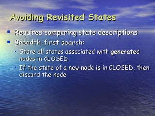
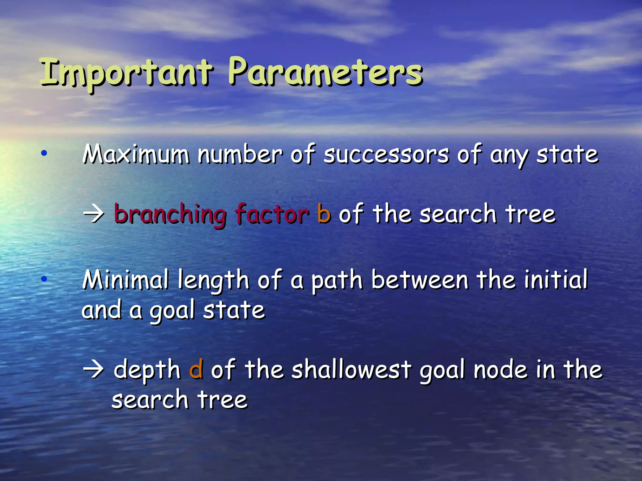
b: branching factor
d: depth of shallowest goal node
m: maximal depth of a leaf node
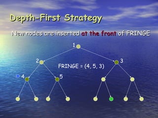
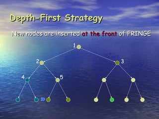
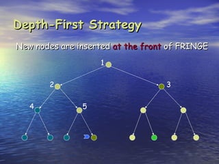
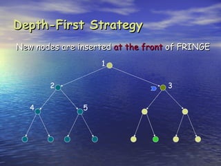
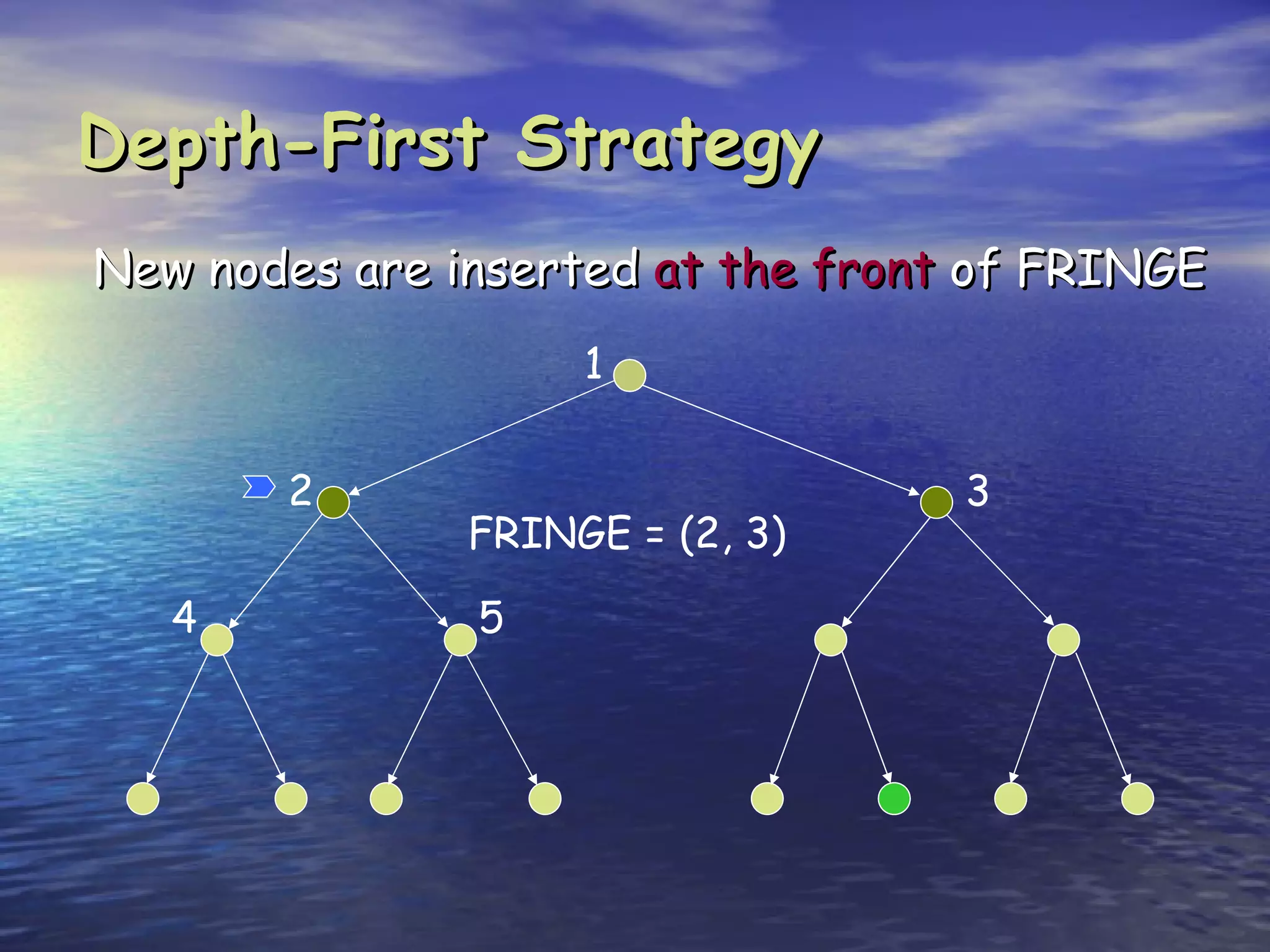
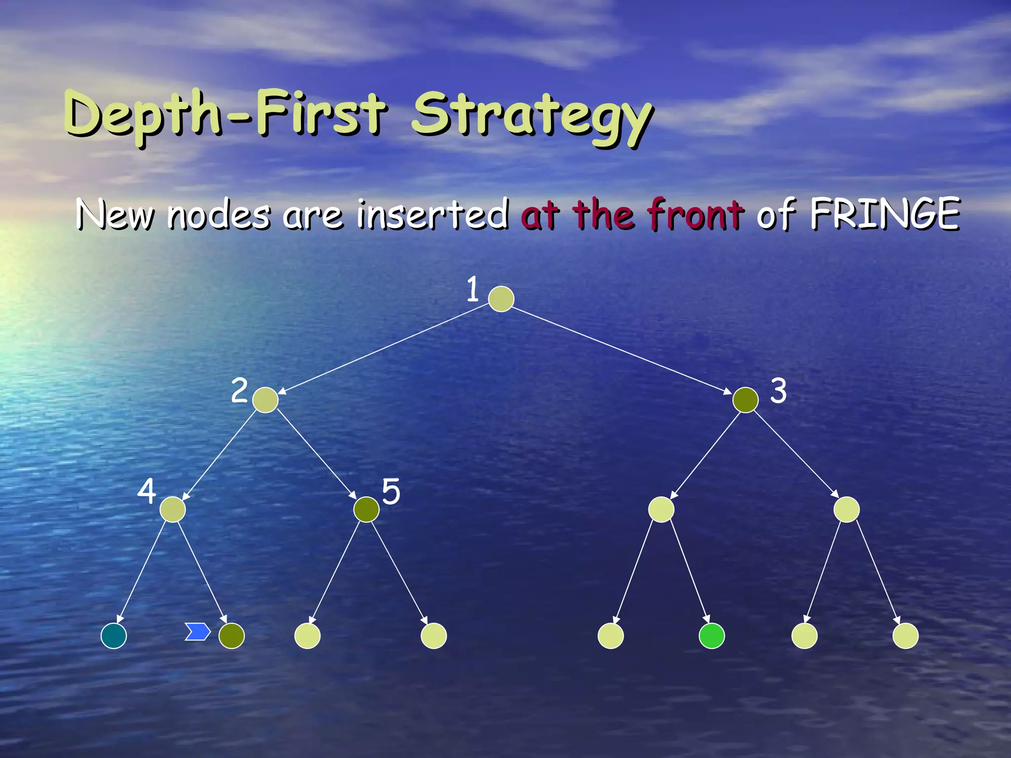
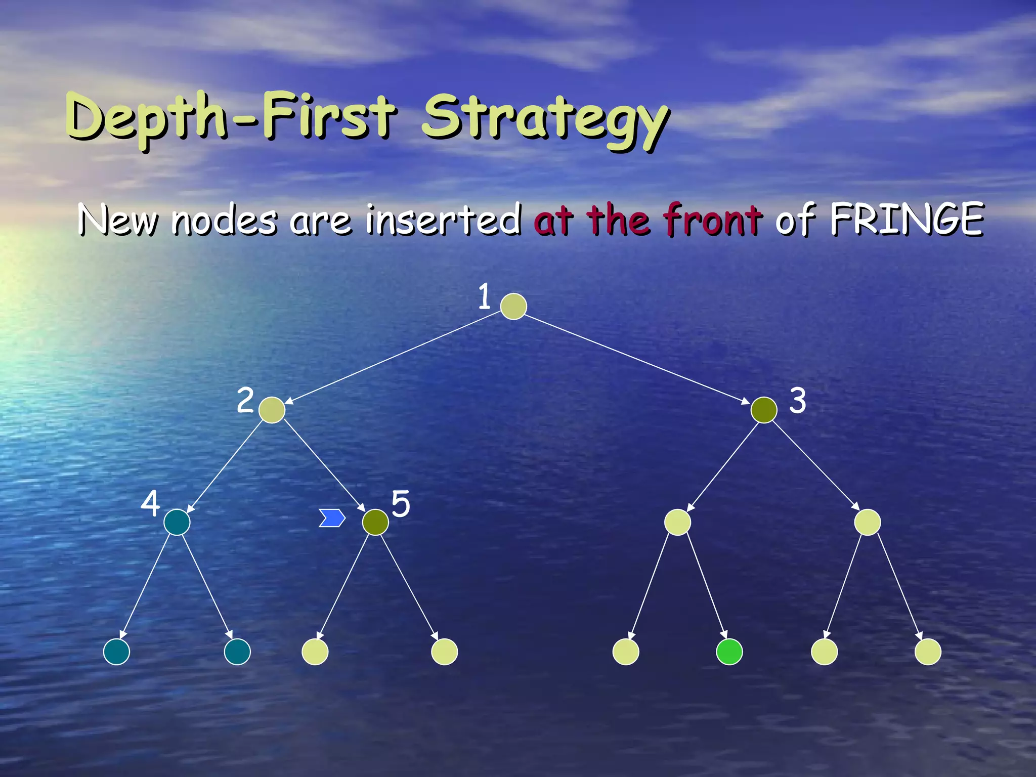
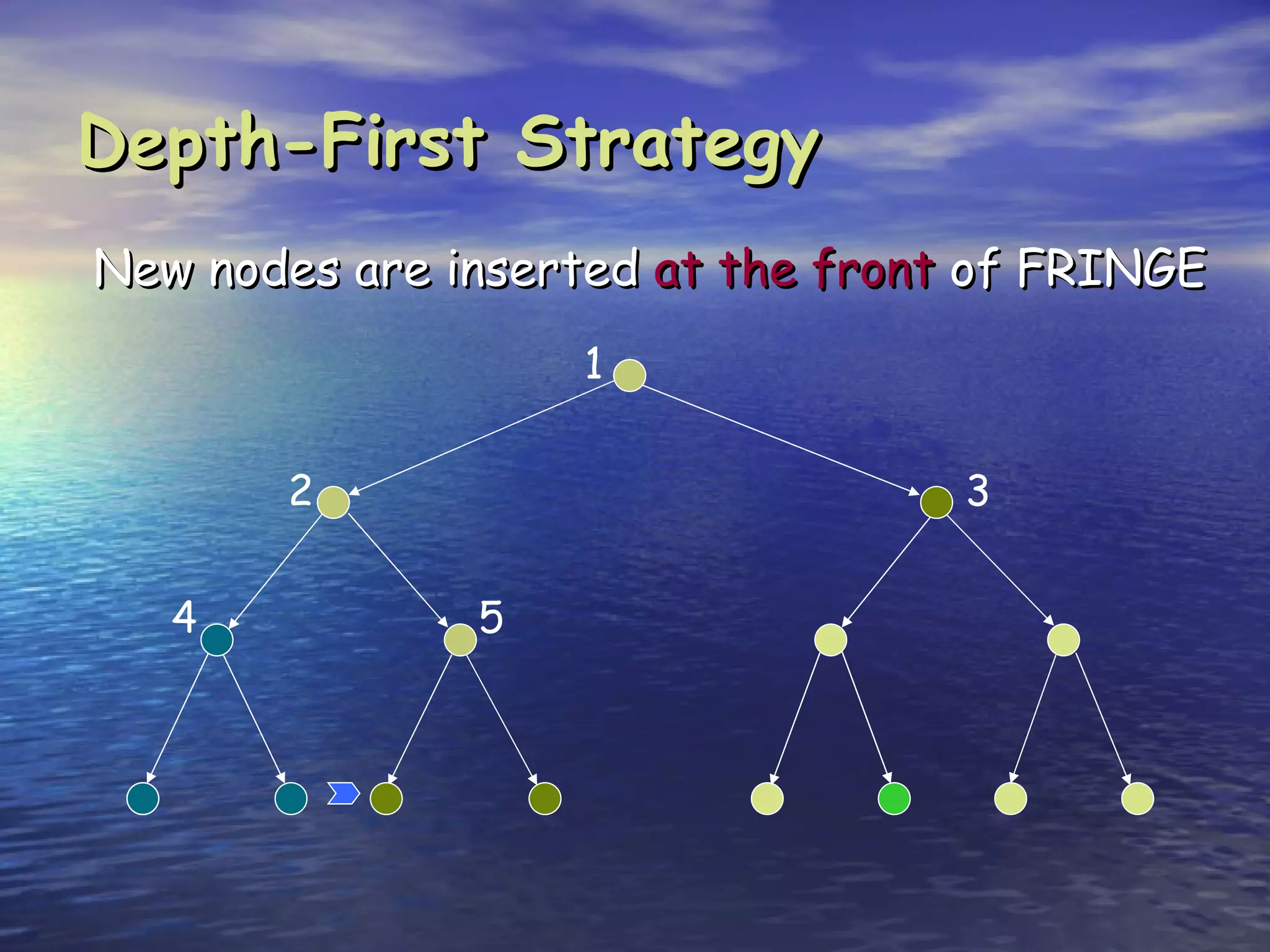
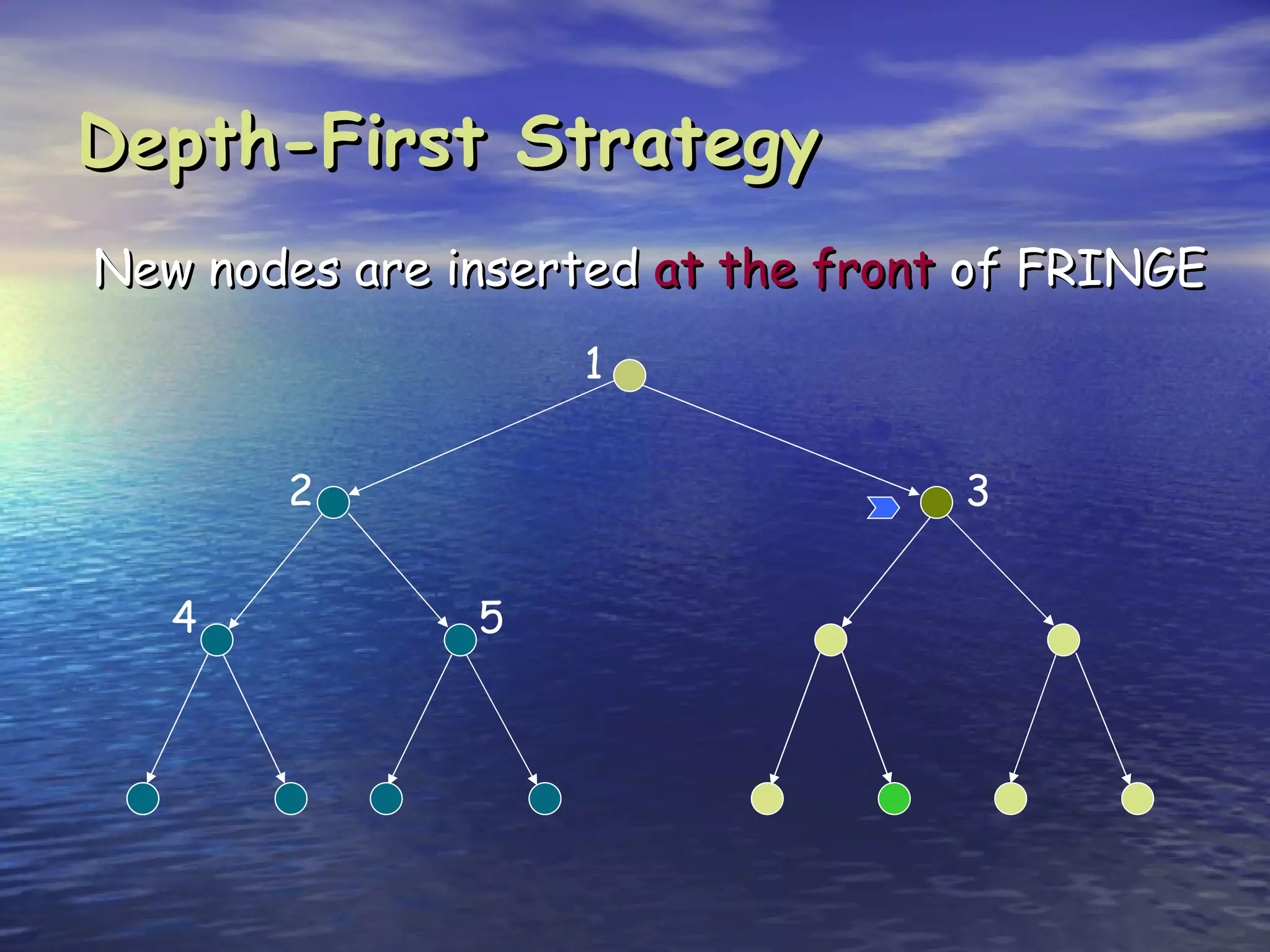
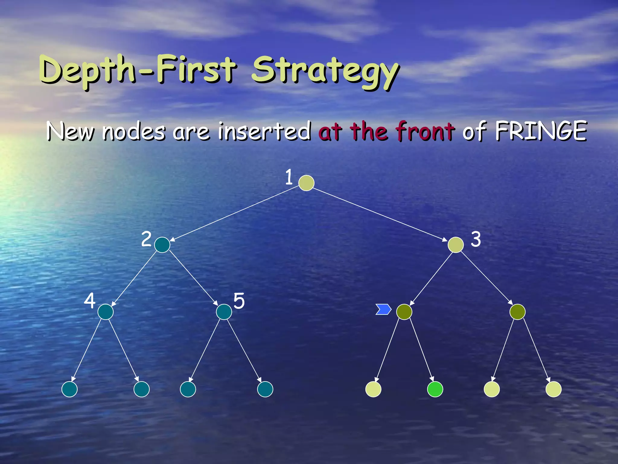
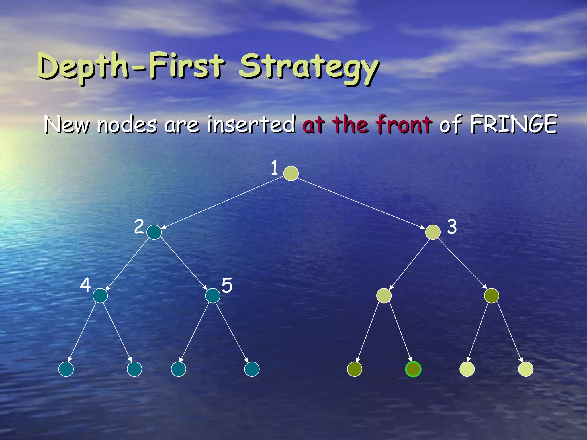
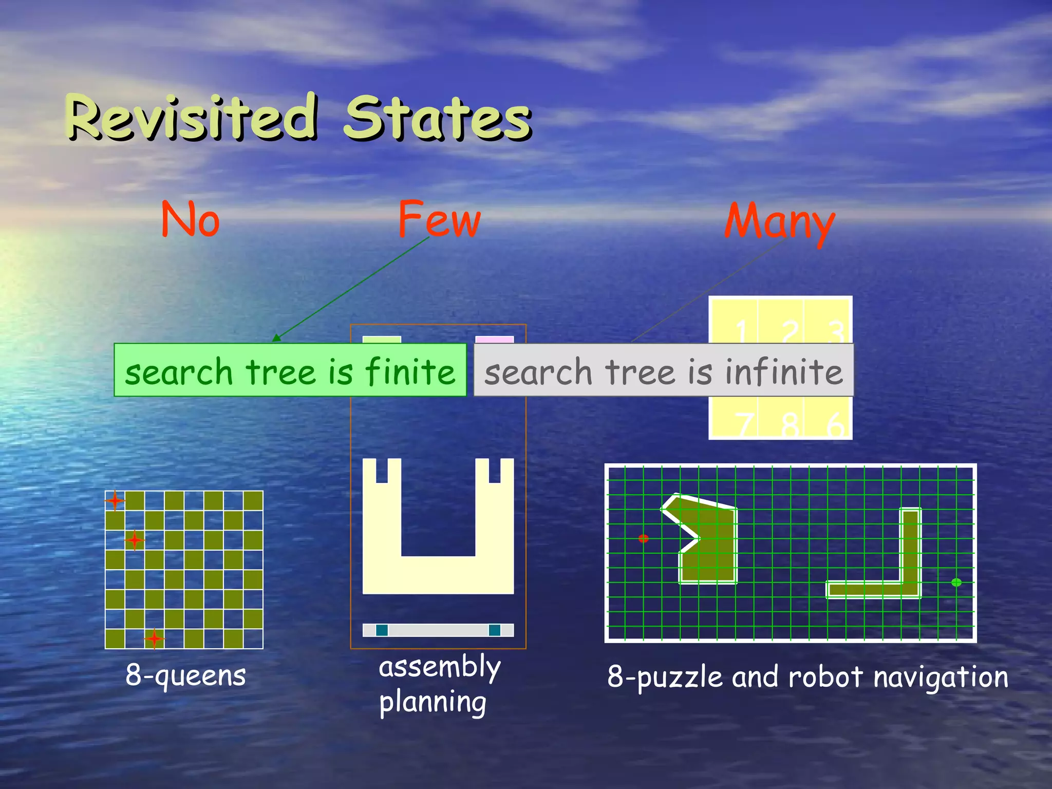
Depth-first search is:
Complete only for finite search tree
Not optimal
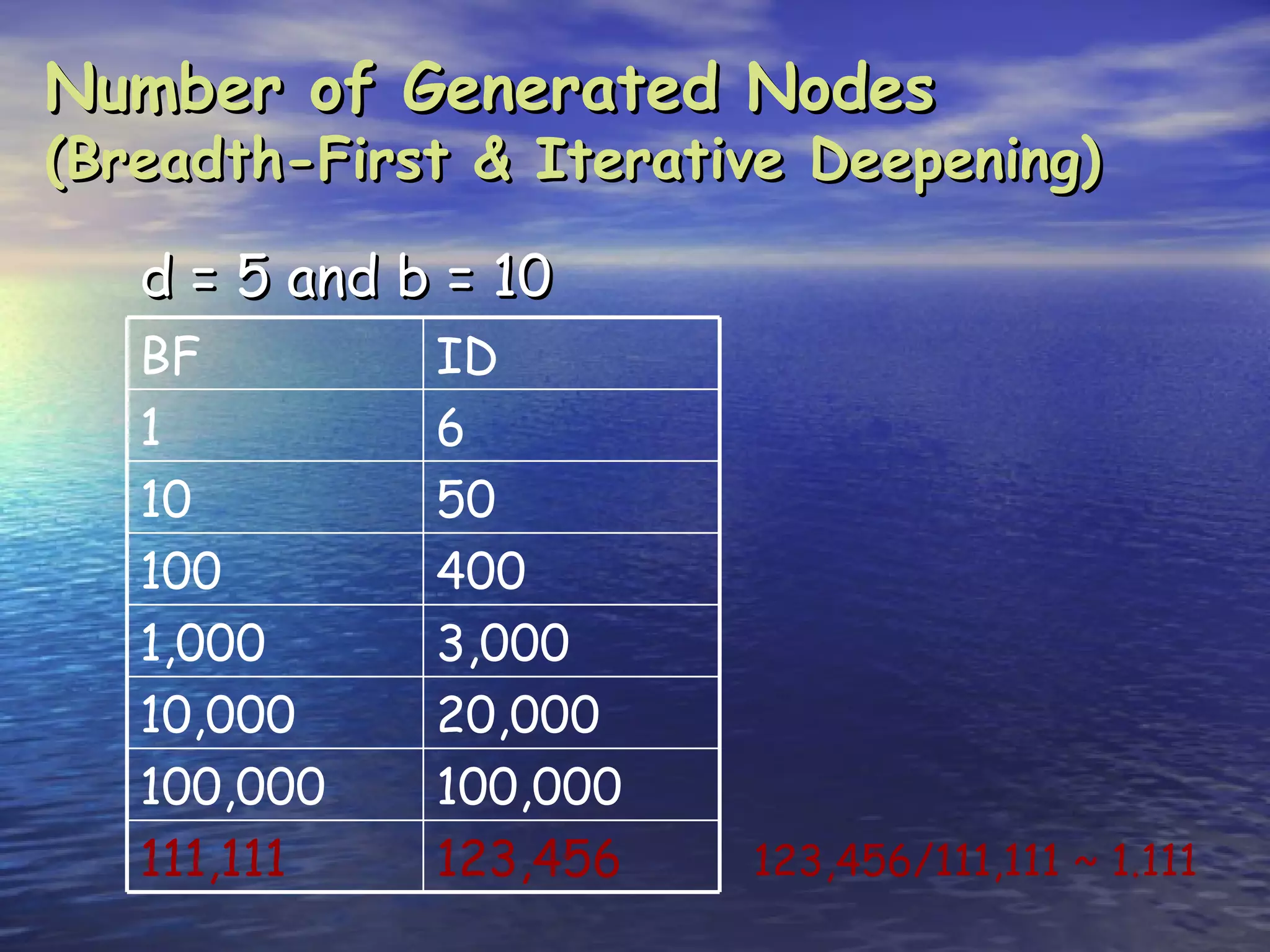
Number of nodes generated:
1 + b + b2 + … + bm = O(bm)
Time complexity is O(bm)
Space complexity is O(bm) [or O(m)]
[Reminder: Breadth-first requires O(bd) time and space]](https://image.slidesharecdn.com/03searchblind-120428063044-phpapp02/85/03-search-blind-48-320.jpg)


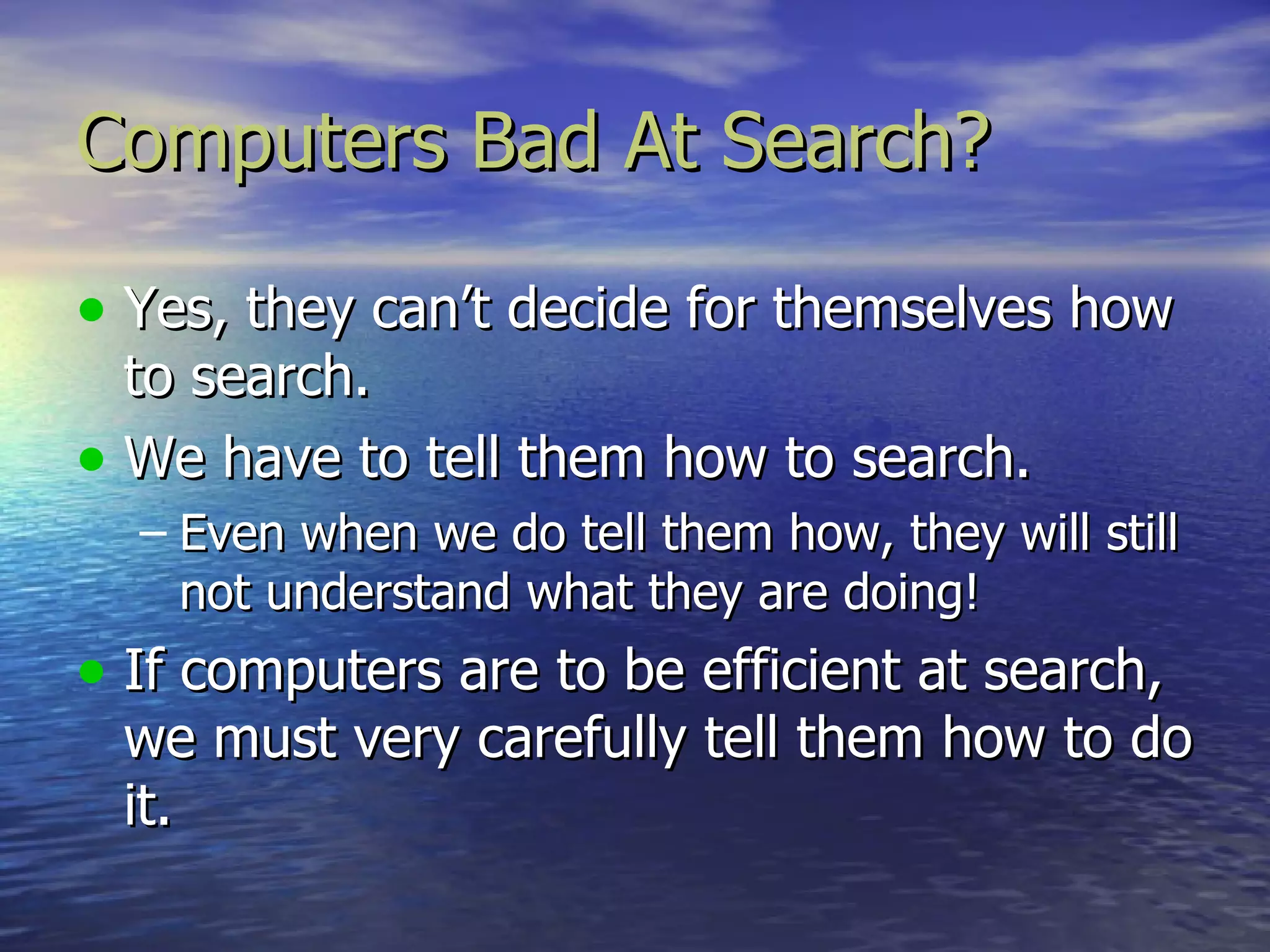


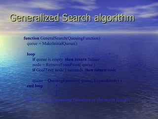
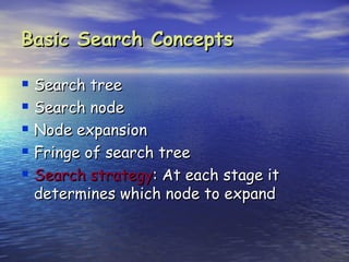
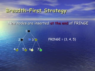
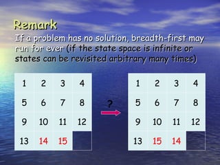
![Performance Measures
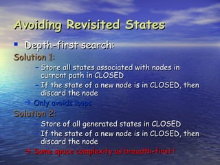
Completeness
A search algorithm is complete if it finds a
solution whenever one exists
[What about the case when no solution exists?]
Optimality
A search algorithm is optimal if it returns an
optimal solution whenever a solution exists
Complexity
It measures the time and amount of memory
required by the algorithm](https://image.slidesharecdn.com/03searchblind-120428063044-phpapp02/75/03-search-blind-21-2048.jpg)


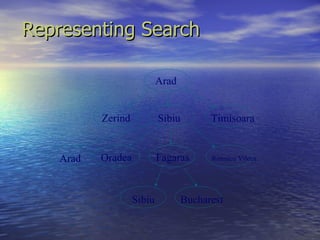
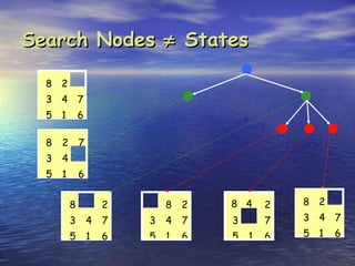
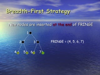
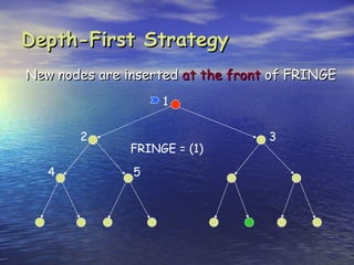
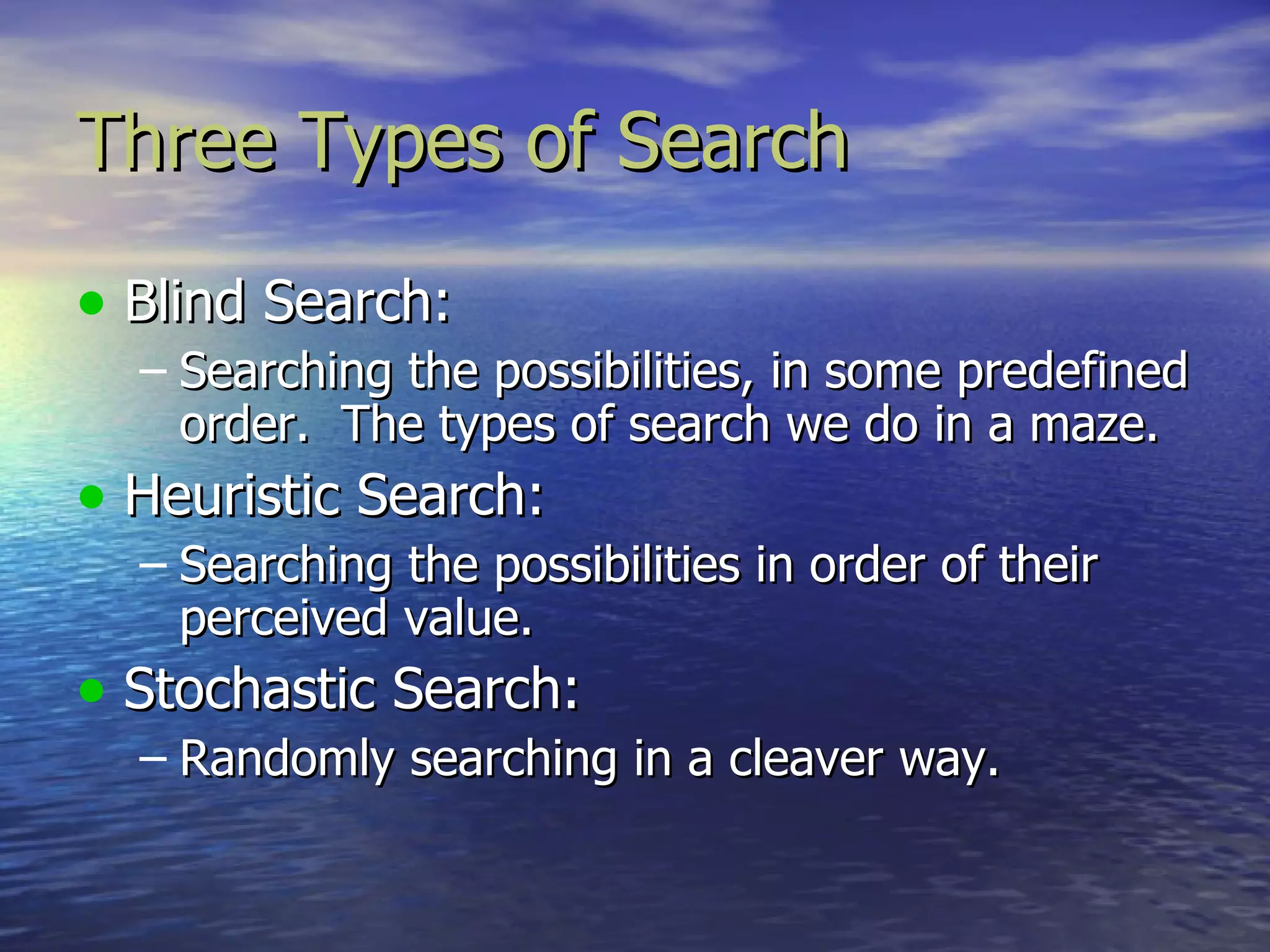
![Evaluation
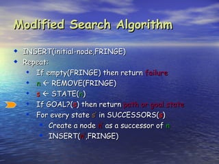
b: branching factor
d: depth of shallowest goal node
m: maximal depth of a leaf node
Depth-first search is:
Complete only for finite search tree
Not optimal
Number of nodes generated:
1 + b + b2 + … + bm = O(bm)
Time complexity is O(bm)
Space complexity is O(bm) [or O(m)]
[Reminder: Breadth-first requires O(bd) time and space]](https://image.slidesharecdn.com/03searchblind-120428063044-phpapp02/75/03-search-blind-48-2048.jpg)


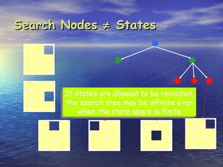
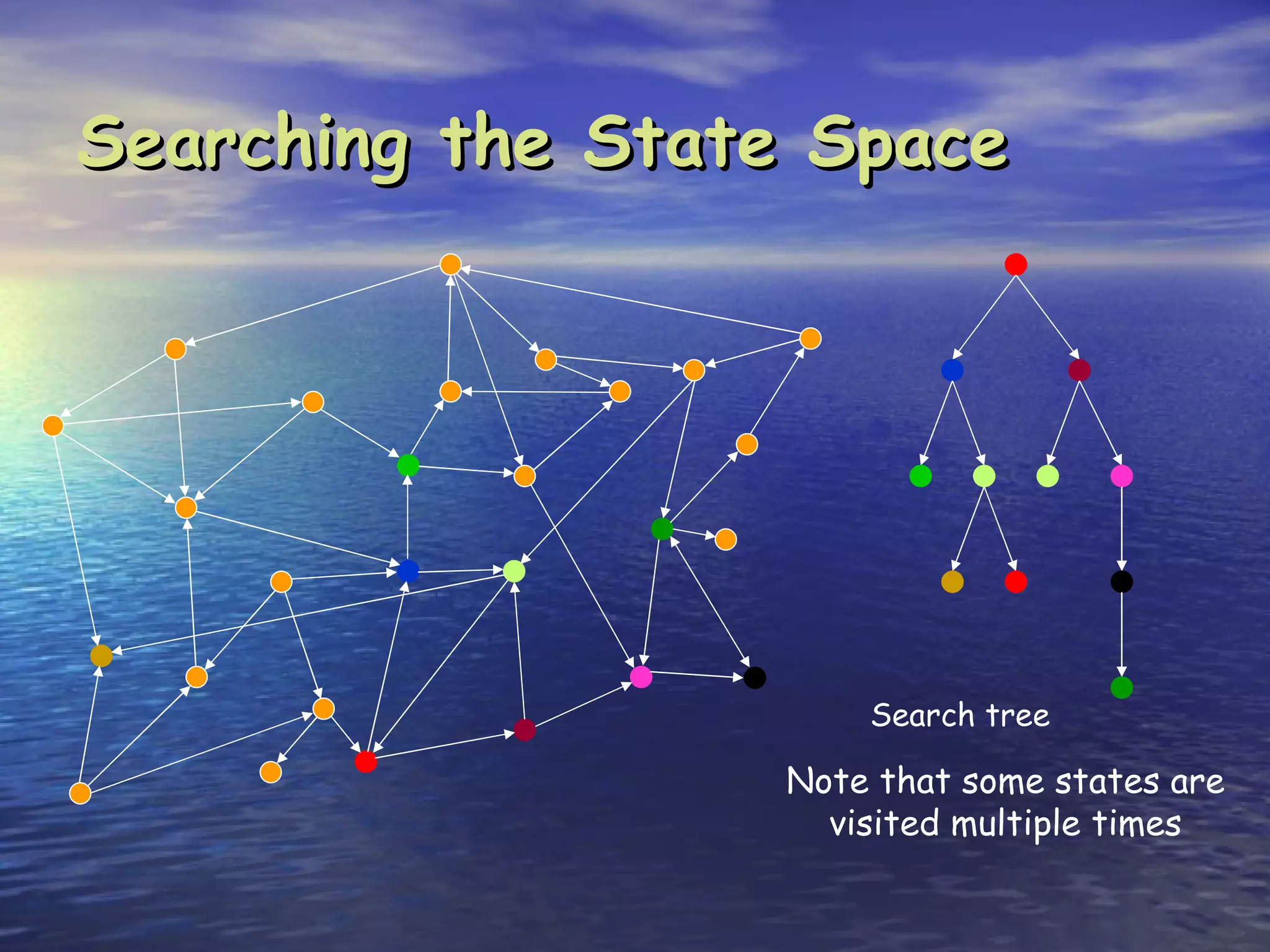
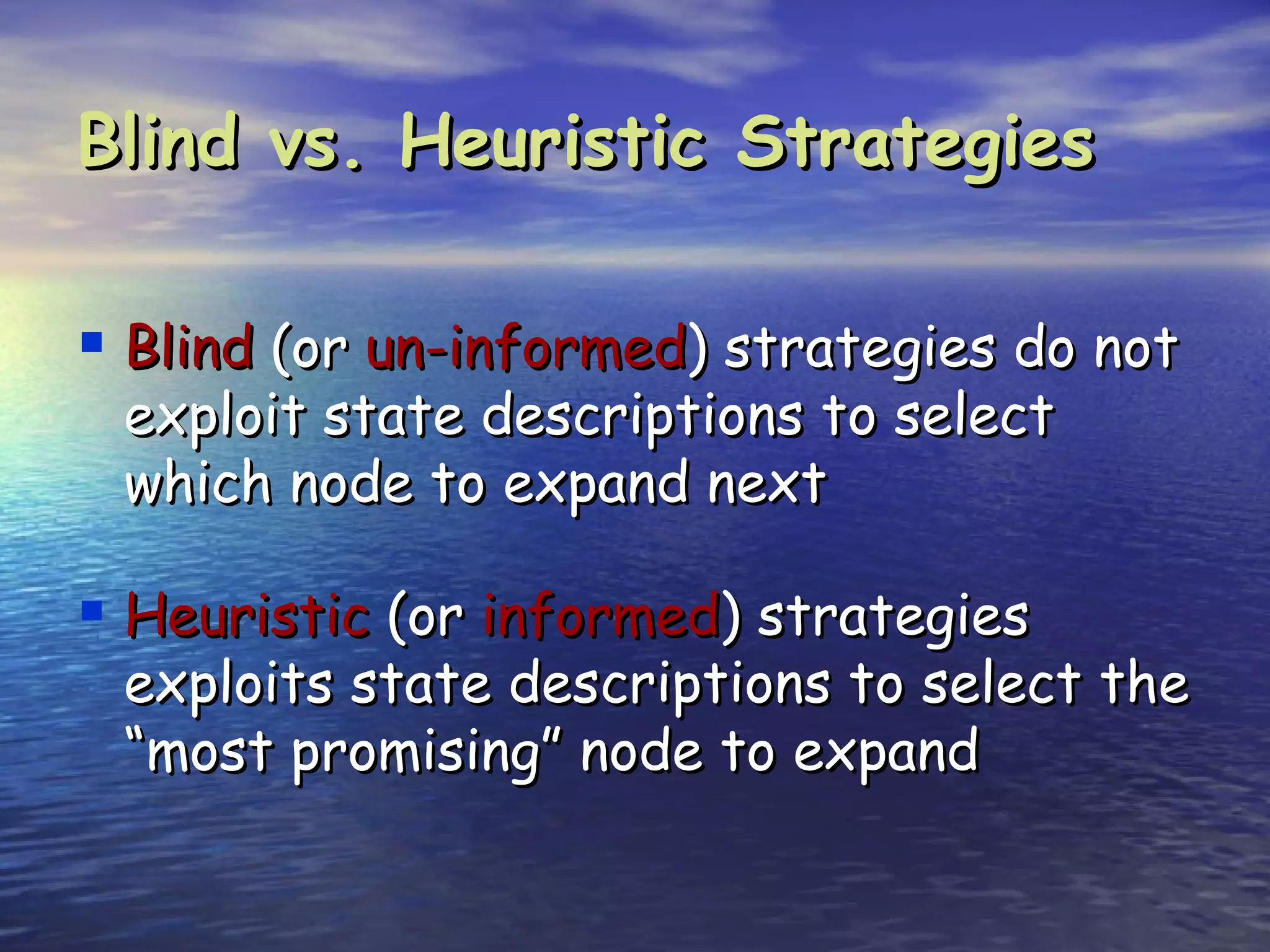
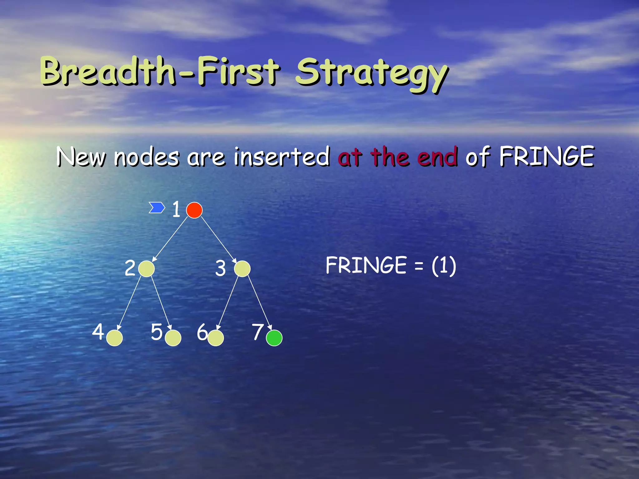
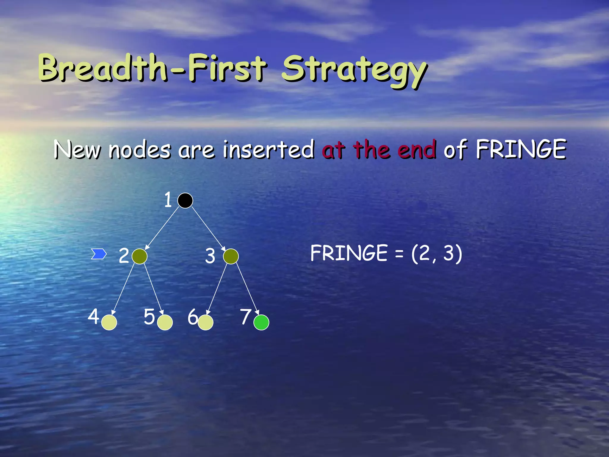
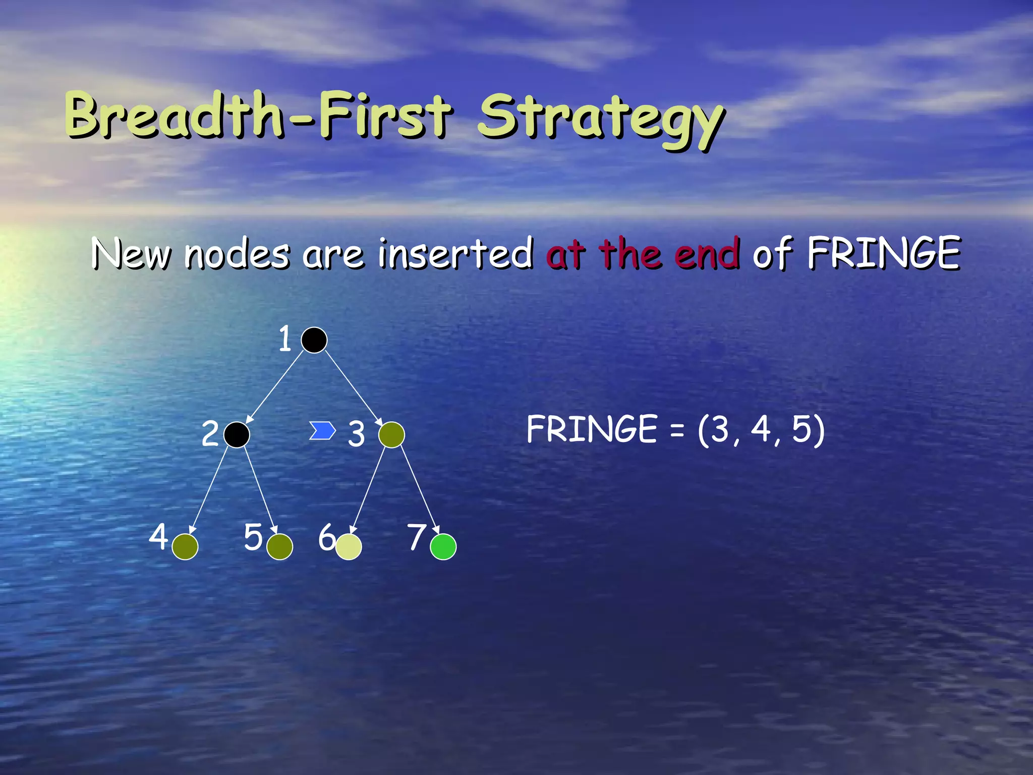
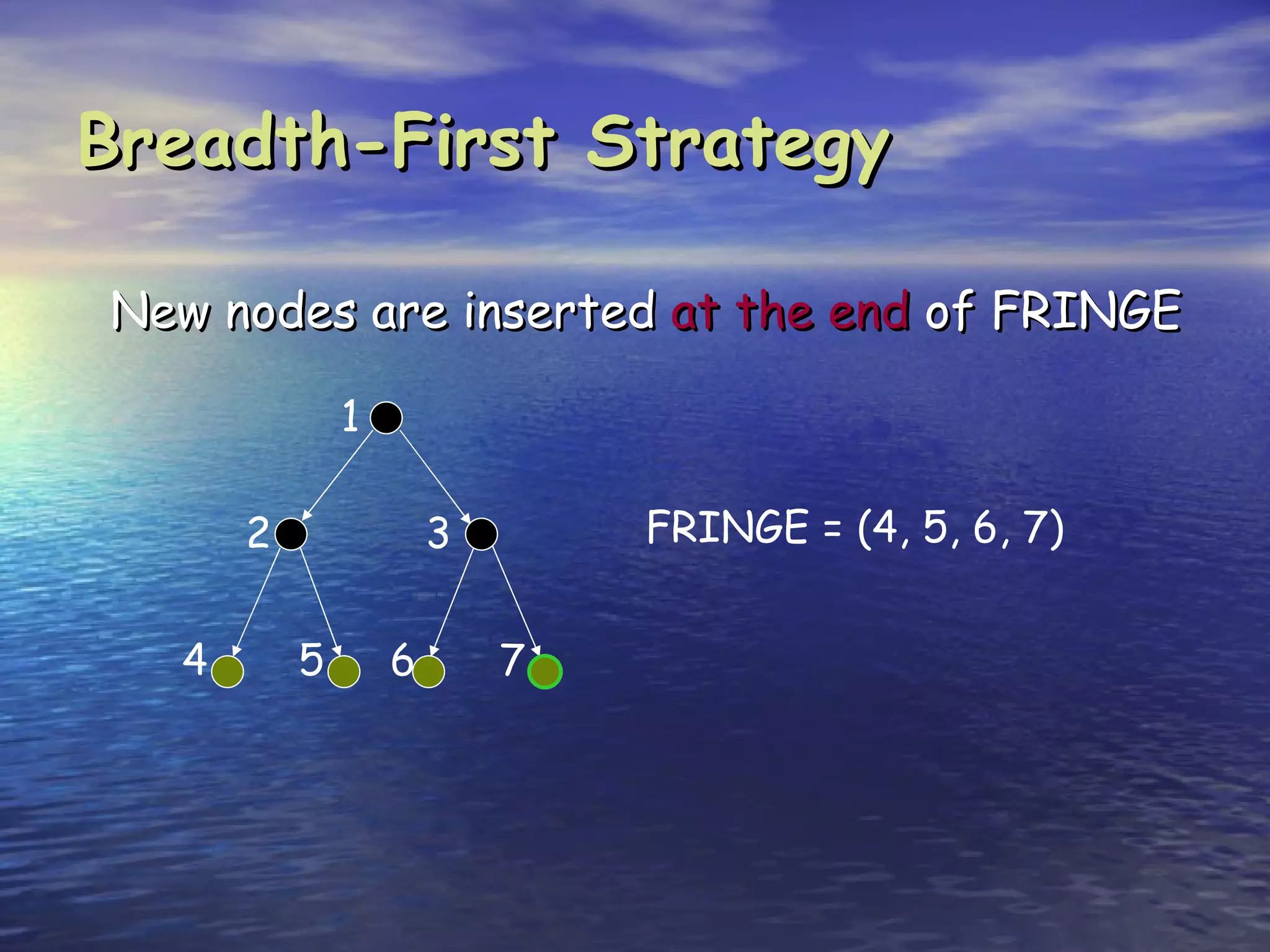
Search is the process of methodically examining potential solutions to find the best one. Computers are not naturally good at search, but can be made efficient through careful programming. There are three main types of search: blind search which examines possibilities in a predefined order, heuristic search which examines possibilities in order of perceived value, and stochastic search which examines possibilities randomly in a clever way. Key aspects of search include completeness (finding a solution if it exists), optimality (finding the best solution), and complexity (resources like time and memory required). Common search strategies include breadth-first, depth-first, and iterative deepening.


