2
Divide-and-conquer algorithms
Divide-and-conquer algorithms
Wehave seen four divide-and-conquer algorithms:
– Binary search
– Depth-first tree traversals
– Merge sort
– Quick sort
The steps are:
– A larger problem is broken up into smaller problems
– The smaller problems are recursively
– The results are combined together again into a solution
4
Divide-and-conquer algorithms
Divide-and-conquer algorithms
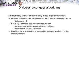
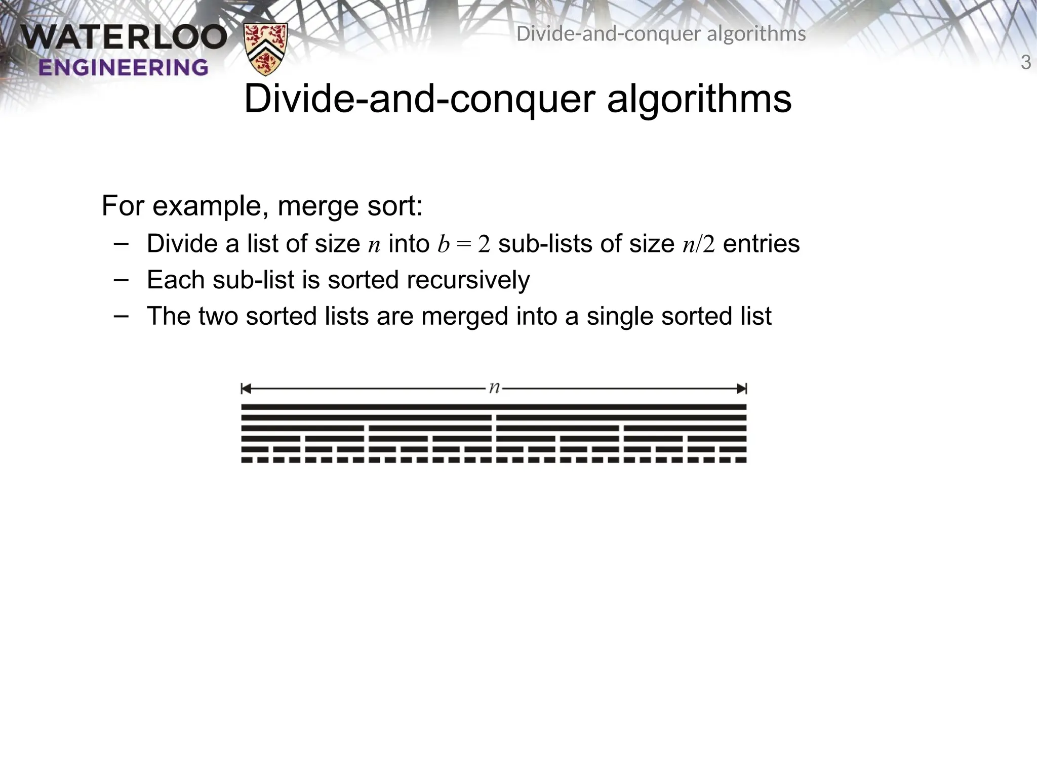
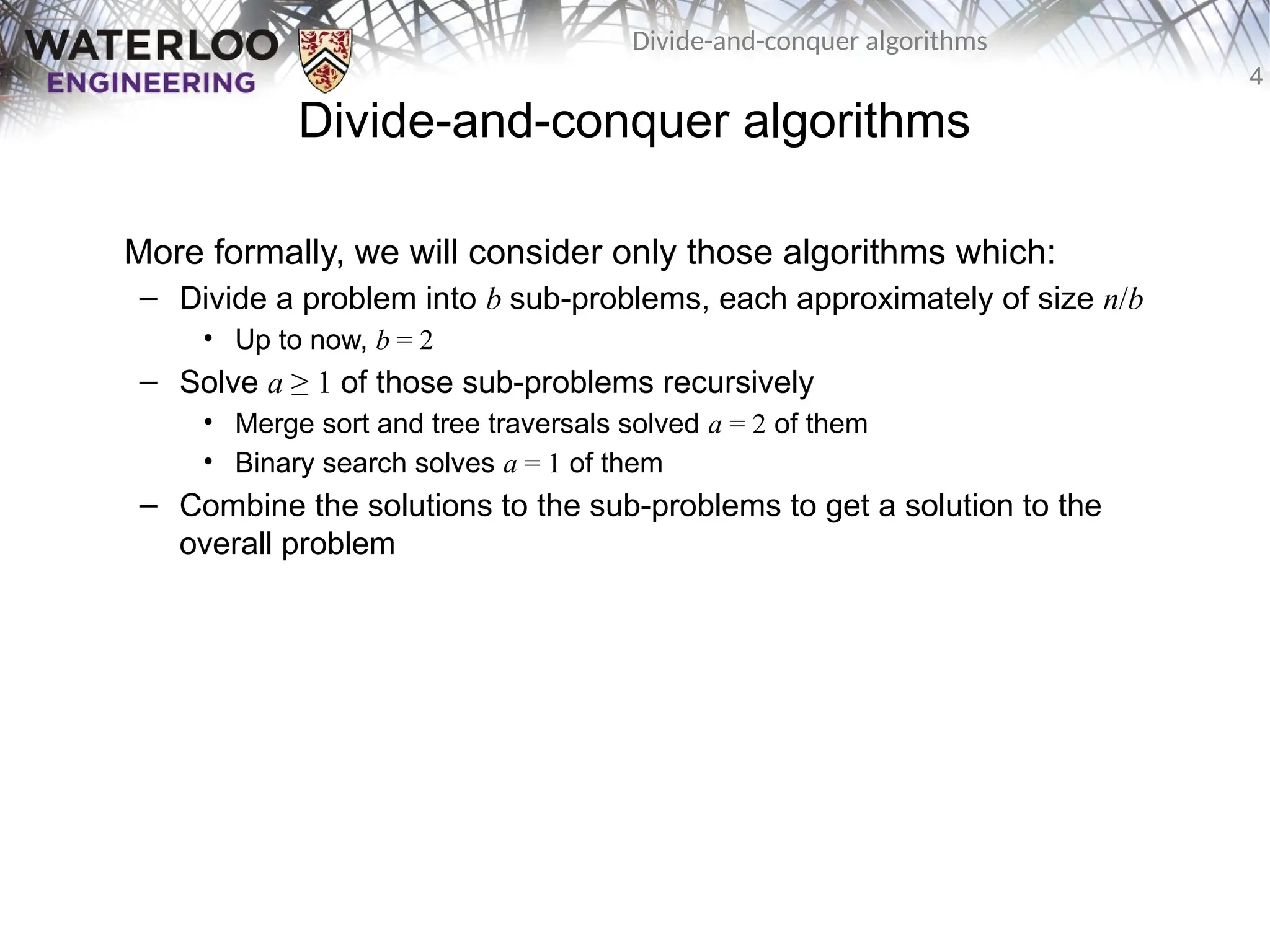
Moreformally, we will consider only those algorithms which:
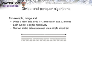
– Divide a problem into b sub-problems, each approximately of size n/b
• Up to now, b = 2
– Solve a ≥ 1 of those sub-problems recursively
• Merge sort and tree traversals solved a = 2 of them
• Binary search solves a = 1 of them
– Combine the solutions to the sub-problems to get a solution to the
overall problem
5.
5
Divide-and-conquer algorithms
Divide-and-conquer algorithms
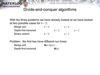
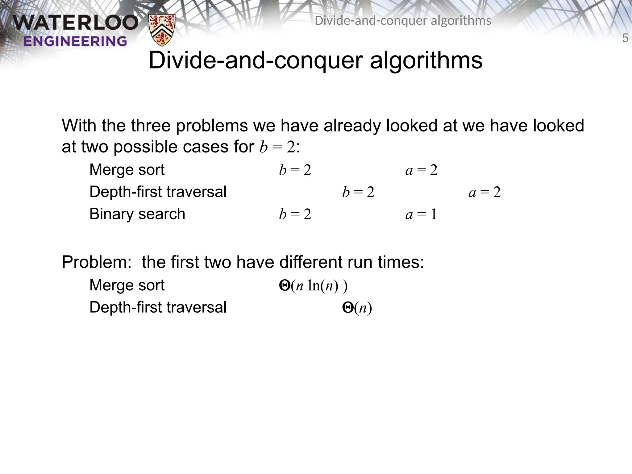
Withthe three problems we have already looked at we have looked
at two possible cases for b = 2:
Merge sort b = 2 a = 2
Depth-first traversal b = 2 a = 2
Binary search b = 2 a = 1
Problem: the first two have different run times:
Merge sort Q(n ln(n) )
Depth-first traversal Q(n)
6.
6
Divide-and-conquer algorithms
Divide-and-conquer algorithms
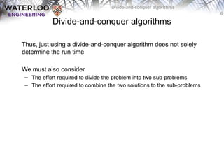
Thus,just using a divide-and-conquer algorithm does not solely
determine the run time
We must also consider
– The effort required to divide the problem into two sub-problems
– The effort required to combine the two solutions to the sub-problems
7.
7
Divide-and-conquer algorithms
Divide-and-conquer algorithms
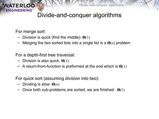
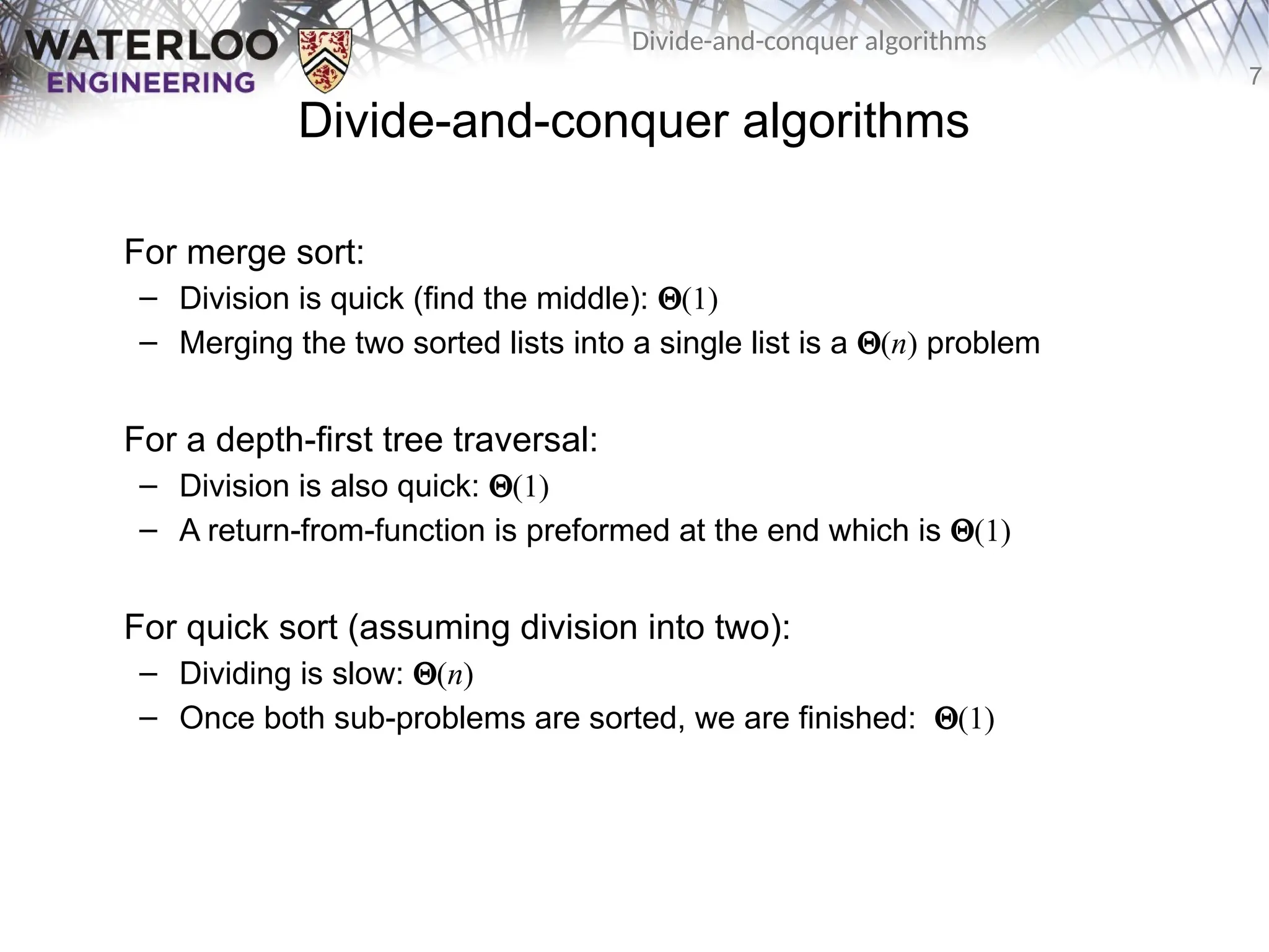
Formerge sort:
– Division is quick (find the middle): Q(1)
– Merging the two sorted lists into a single list is a Q(n) problem
For a depth-first tree traversal:
– Division is also quick: Q(1)
– A return-from-function is preformed at the end which is Q(1)
For quick sort (assuming division into two):
– Dividing is slow: Q(n)
– Once both sub-problems are sorted, we are finished: Q(1)
8.
8
Divide-and-conquer algorithms
Divide-and-conquer algorithms
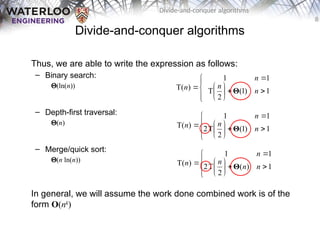
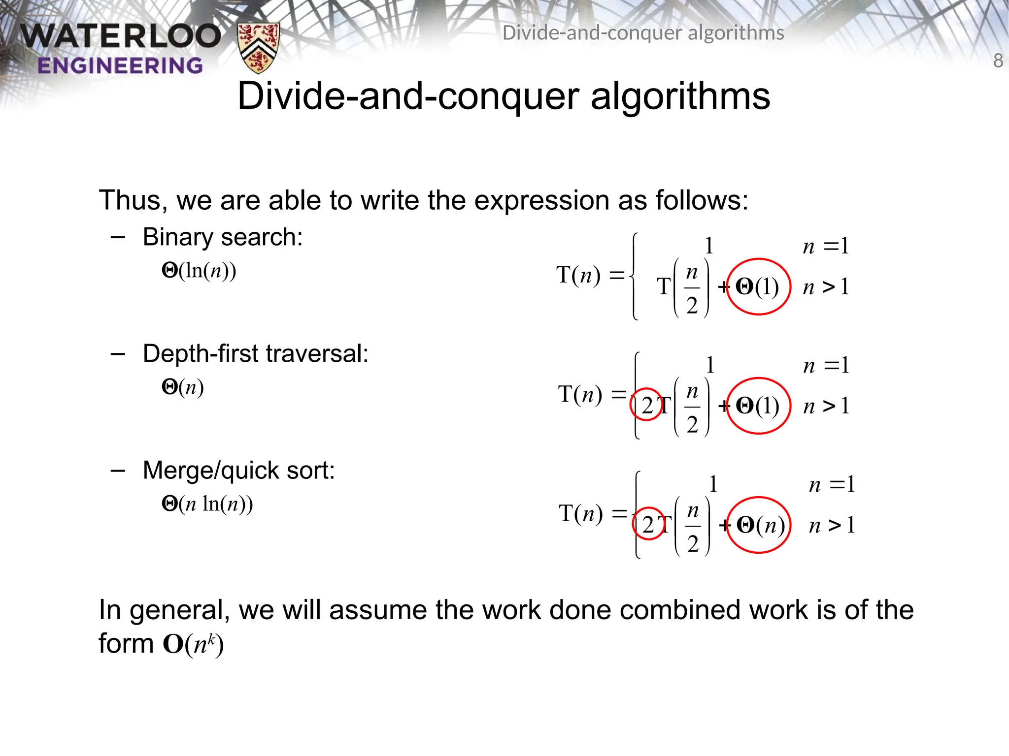
Thus,we are able to write the expression as follows:
– Binary search:
Q(ln(n))
– Depth-first traversal:
Q(n)
– Merge/quick sort:
Q(n ln(n))
In general, we will assume the work done combined work is of the
form O(nk
)
1
)
1
(
2
T
1
1
)
T( n
n
n
n Θ
1
)
1
(
2
T
2
1
1
)
T( n
n
n
n Θ
1
)
(
2
T
2
1
1
)
T( n
n
n
n
n Θ
9.
9
Divide-and-conquer algorithms
Divide-and-conquer algorithms
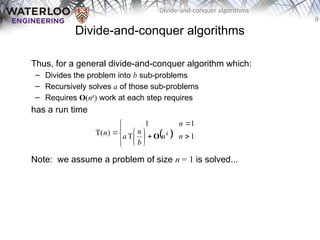
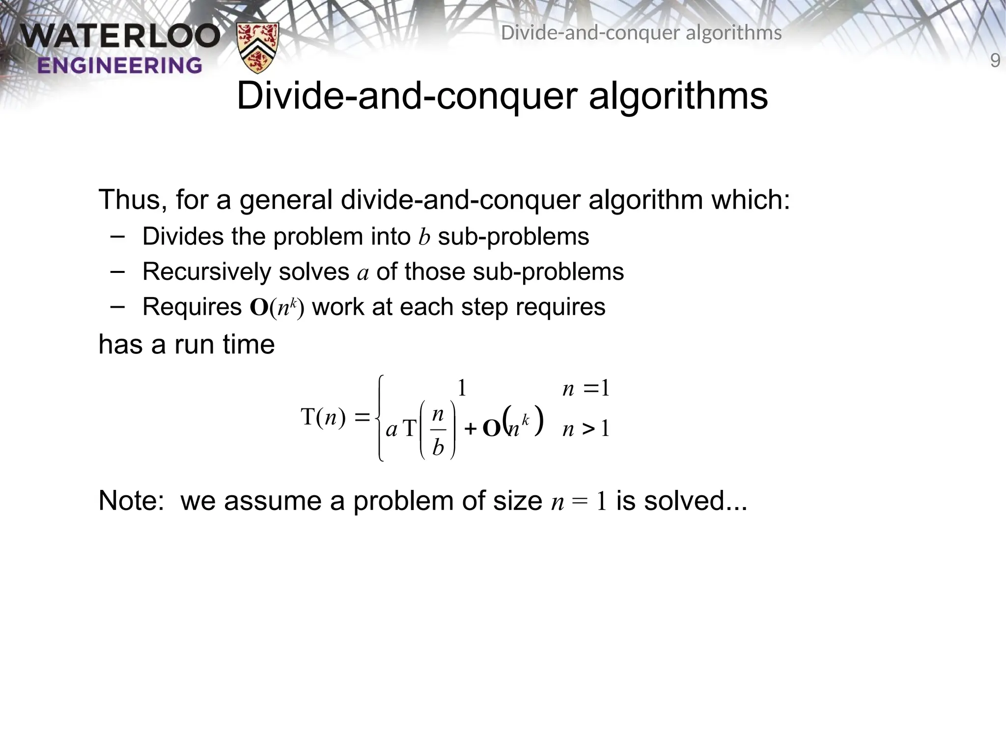
Thus,for a general divide-and-conquer algorithm which:
– Divides the problem into b sub-problems
– Recursively solves a of those sub-problems
– Requires O(nk
) work at each step requires
has a run time
Note: we assume a problem of size n = 1 is solved...
1
T
1
1
)
T( n
n
b
n
a
n
n k
O
11
Divide-and-conquer algorithms
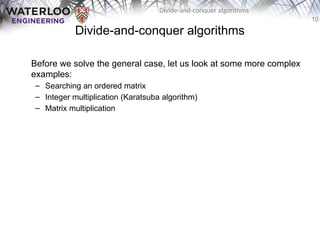
Searching anordered matrix
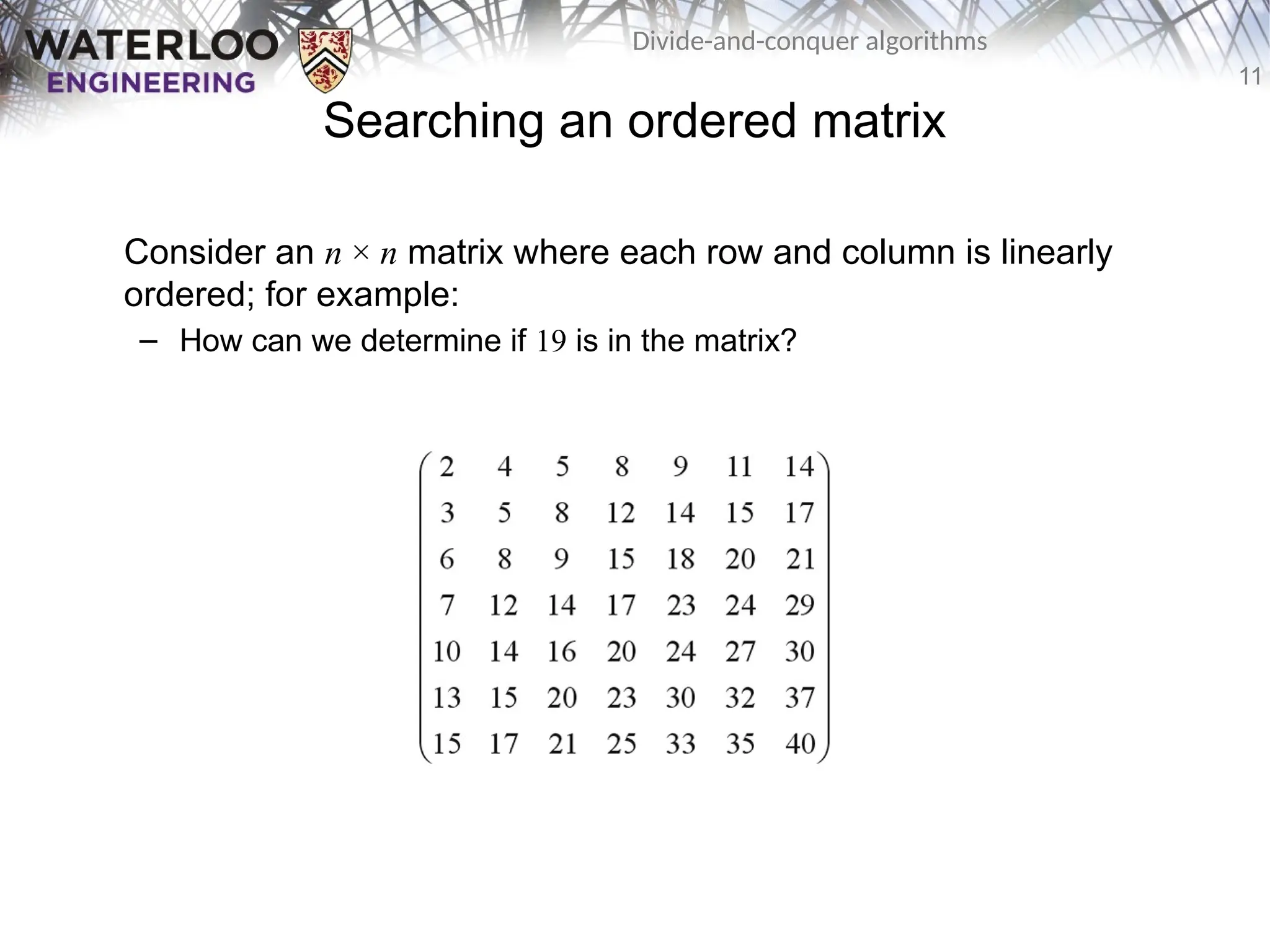
Consider an n × n matrix where each row and column is linearly
ordered; for example:
– How can we determine if 19 is in the matrix?
12.
12
Divide-and-conquer algorithms
Searching anordered matrix
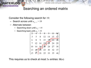
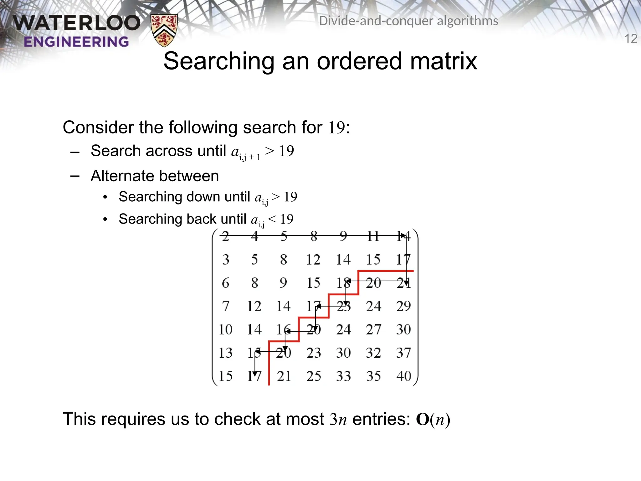
Consider the following search for 19:
– Search across until ai,j + 1 > 19
– Alternate between
• Searching down until ai,j > 19
• Searching back until ai,j < 19
This requires us to check at most 3n entries: O(n)
13.
13
Divide-and-conquer algorithms
Searching anordered matrix
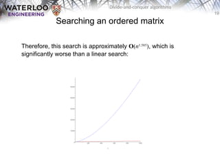
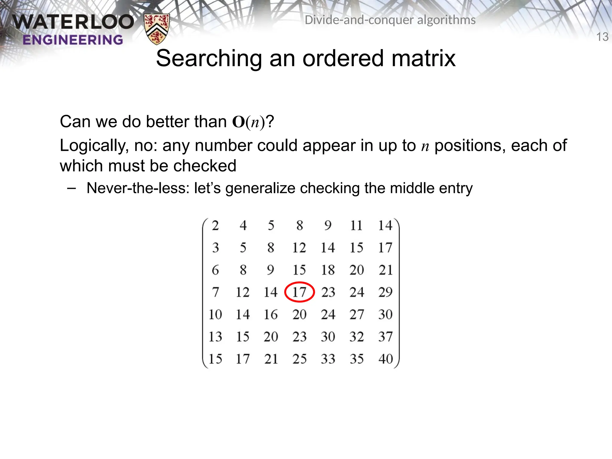
Can we do better than O(n)?
Logically, no: any number could appear in up to n positions, each of
which must be checked
– Never-the-less: let’s generalize checking the middle entry
16
Divide-and-conquer algorithms
Searching anordered matrix
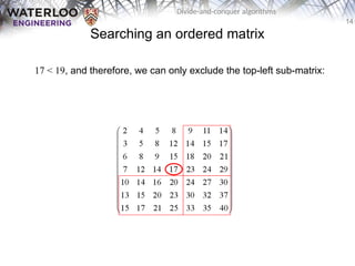
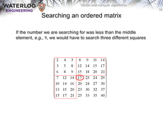
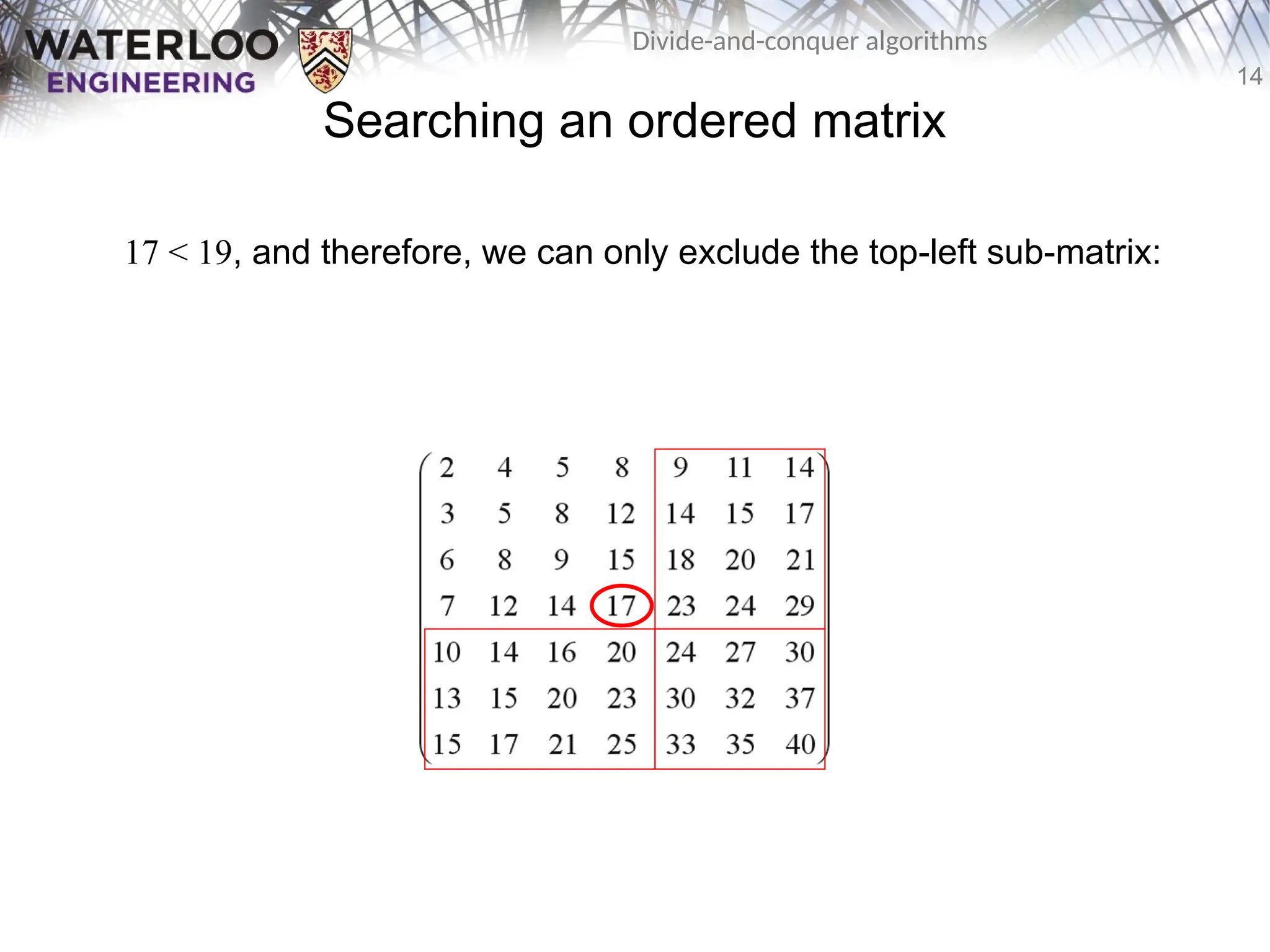
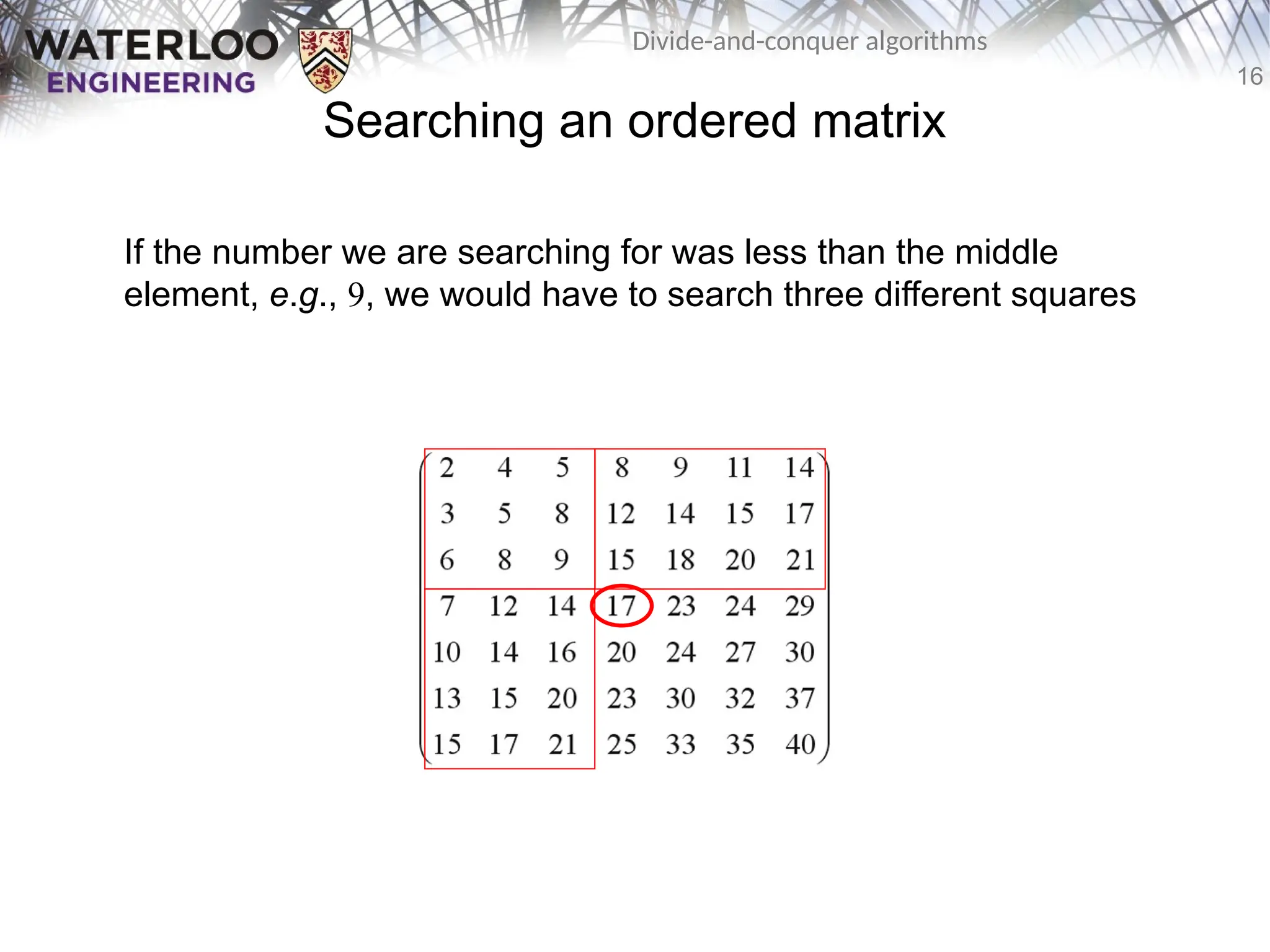
If the number we are searching for was less than the middle
element, e.g., 9, we would have to search three different squares
17.
17
Divide-and-conquer algorithms
Searching anordered matrix
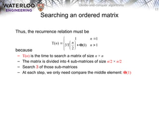
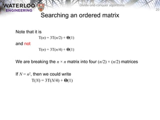
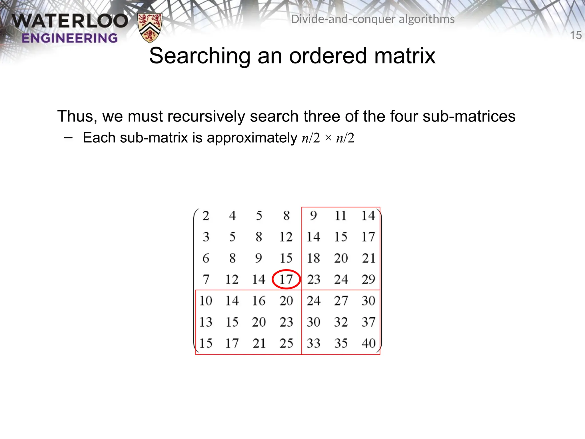
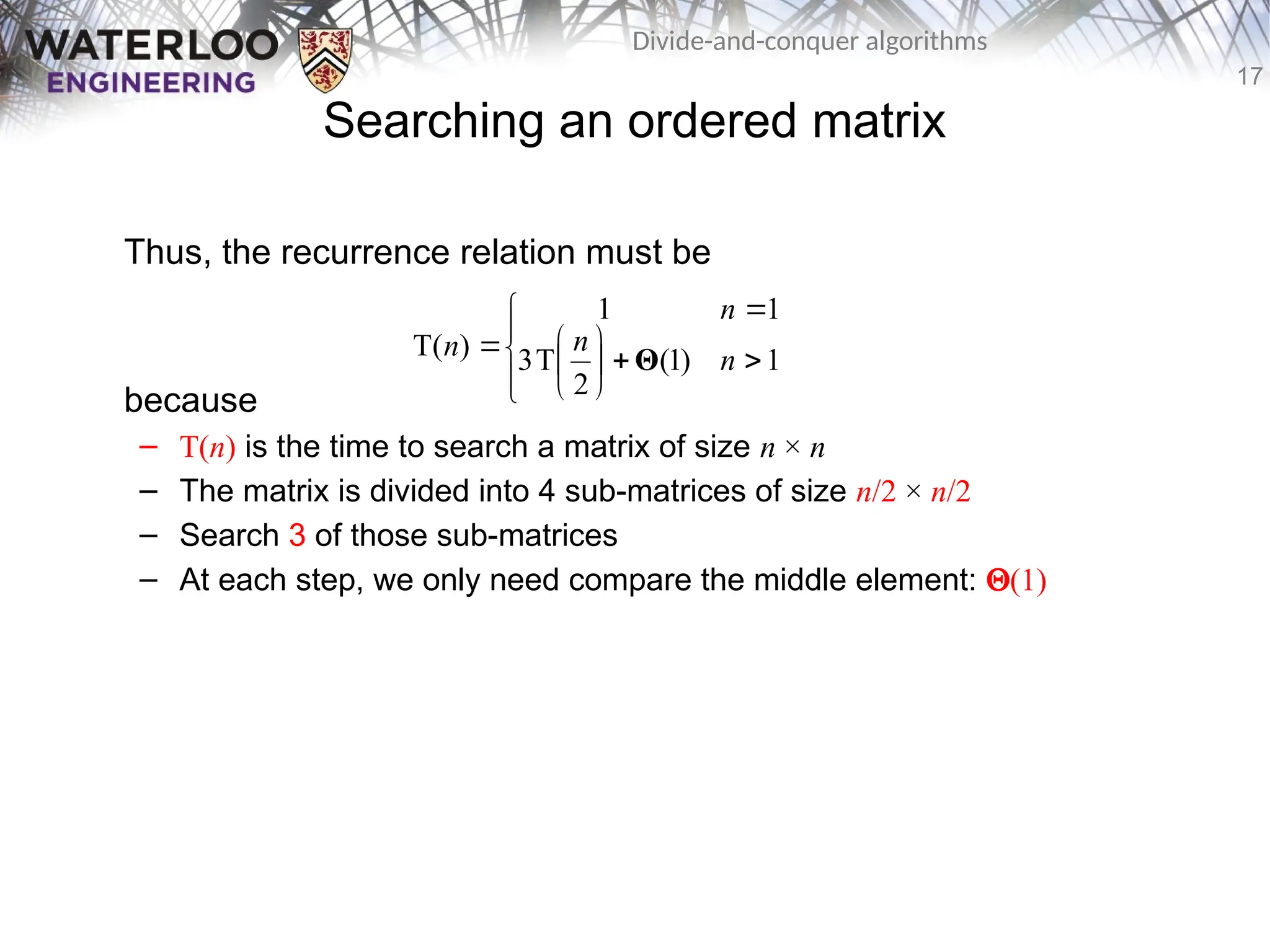
Thus, the recurrence relation must be
because
– T(n) is the time to search a matrix of size n × n
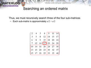
– The matrix is divided into 4 sub-matrices of size n/2 × n/2
– Search 3 of those sub-matrices
– At each step, we only need compare the middle element: Q(1)
1
)
1
(
2
T
3
1
1
)
T( n
n
n
n Θ
18.
18
Divide-and-conquer algorithms
Searching anordered matrix
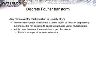
We can solve the recurrence relationship
using Maple:
> rsolve( {T(n) = 3*T(n/2) + 1, T(1) = 1}, T(n) );
> evalf( log[2]( 3 ) );
1
)
1
(
2
T
3
1
1
)
T( n
n
n
n Θ
3
2
n
( )
log2 3 1
2
1.584962501
20
Divide-and-conquer algorithms
Searching anordered matrix
Note that it is
T(n) = 3T(n/2) + Q(1)
and not
T(n) = 3T(n/4) + Q(1)
We are breaking the n × n matrix into four (n/2) × (n/2) matrices
If N = n2
, then we could write
T(N) = 3T(N/4) + Q(1)
21.
21
Divide-and-conquer algorithms
Searching anordered matrix
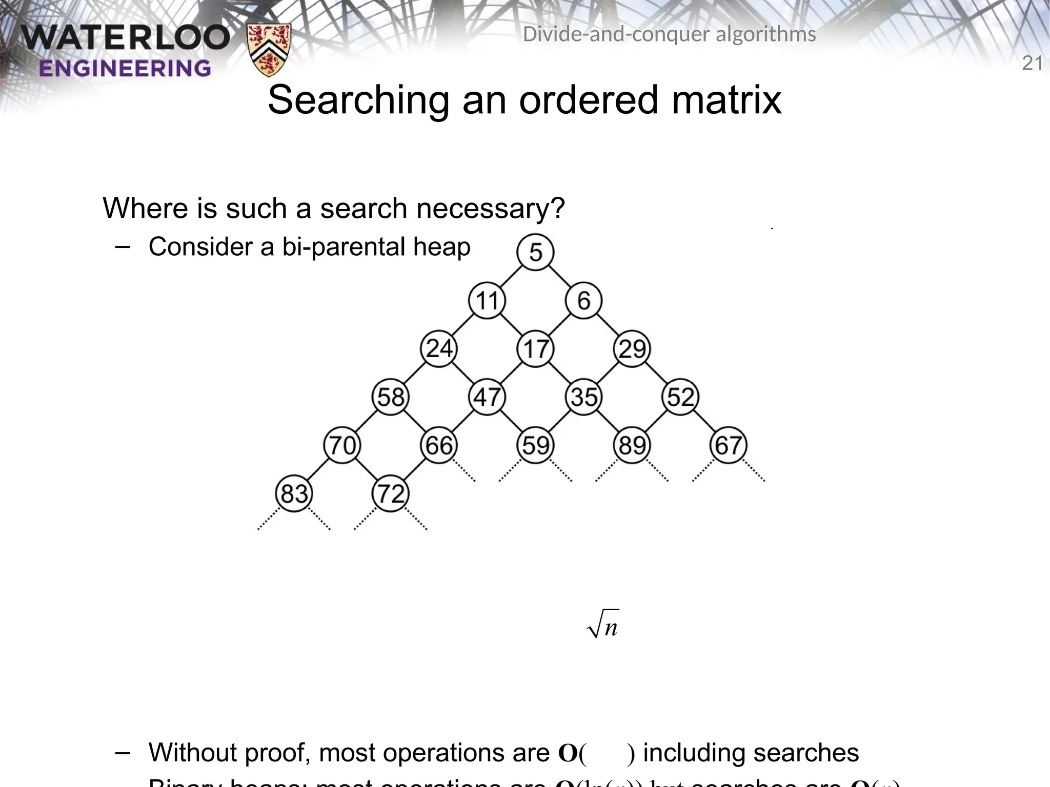
Where is such a search necessary?
– Consider a bi-parental heap
– Without proof, most operations are O( ) including searches
n
22.
22
Divide-and-conquer algorithms
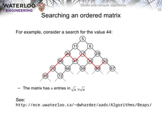
Searching anordered matrix
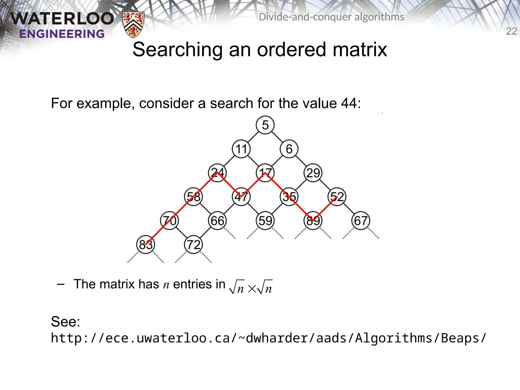
For example, consider a search for the value 44:
– The matrix has n entries in
See:
http://ece.uwaterloo.ca/~dwharder/aads/Algorithms/Beaps/
n n
23.
23
Divide-and-conquer algorithms
Searching anordered matrix
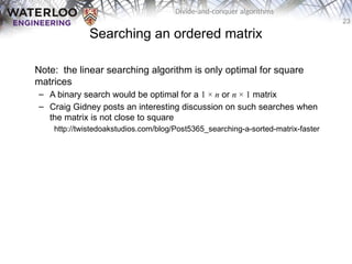
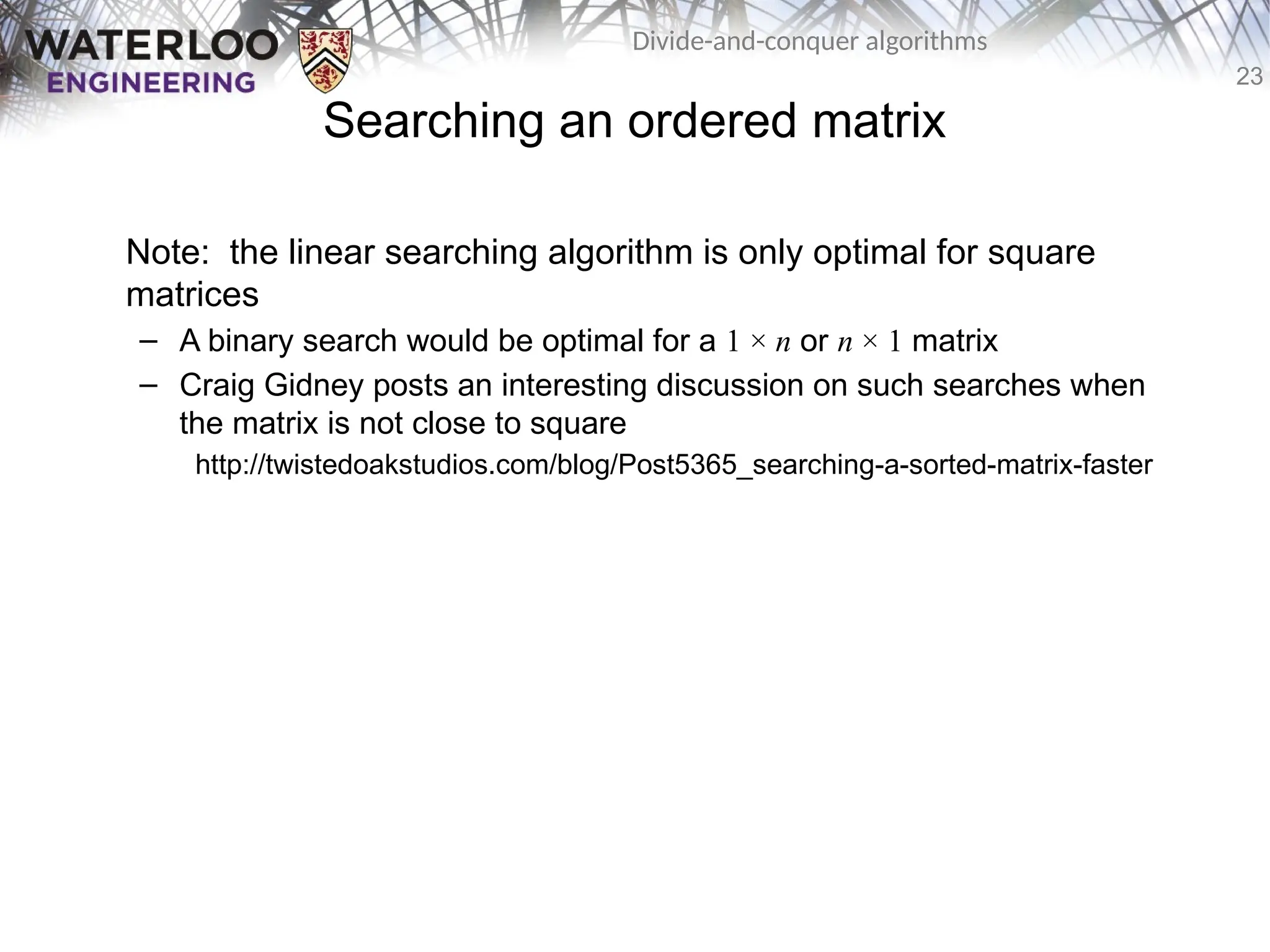
Note: the linear searching algorithm is only optimal for square
matrices
– A binary search would be optimal for a 1 × n or n × 1 matrix
– Craig Gidney posts an interesting discussion on such searches when
the matrix is not close to square
http://twistedoakstudios.com/blog/Post5365_searching-a-sorted-matrix-faster
24.
24
Divide-and-conquer algorithms
Integer multiplication
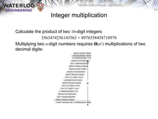
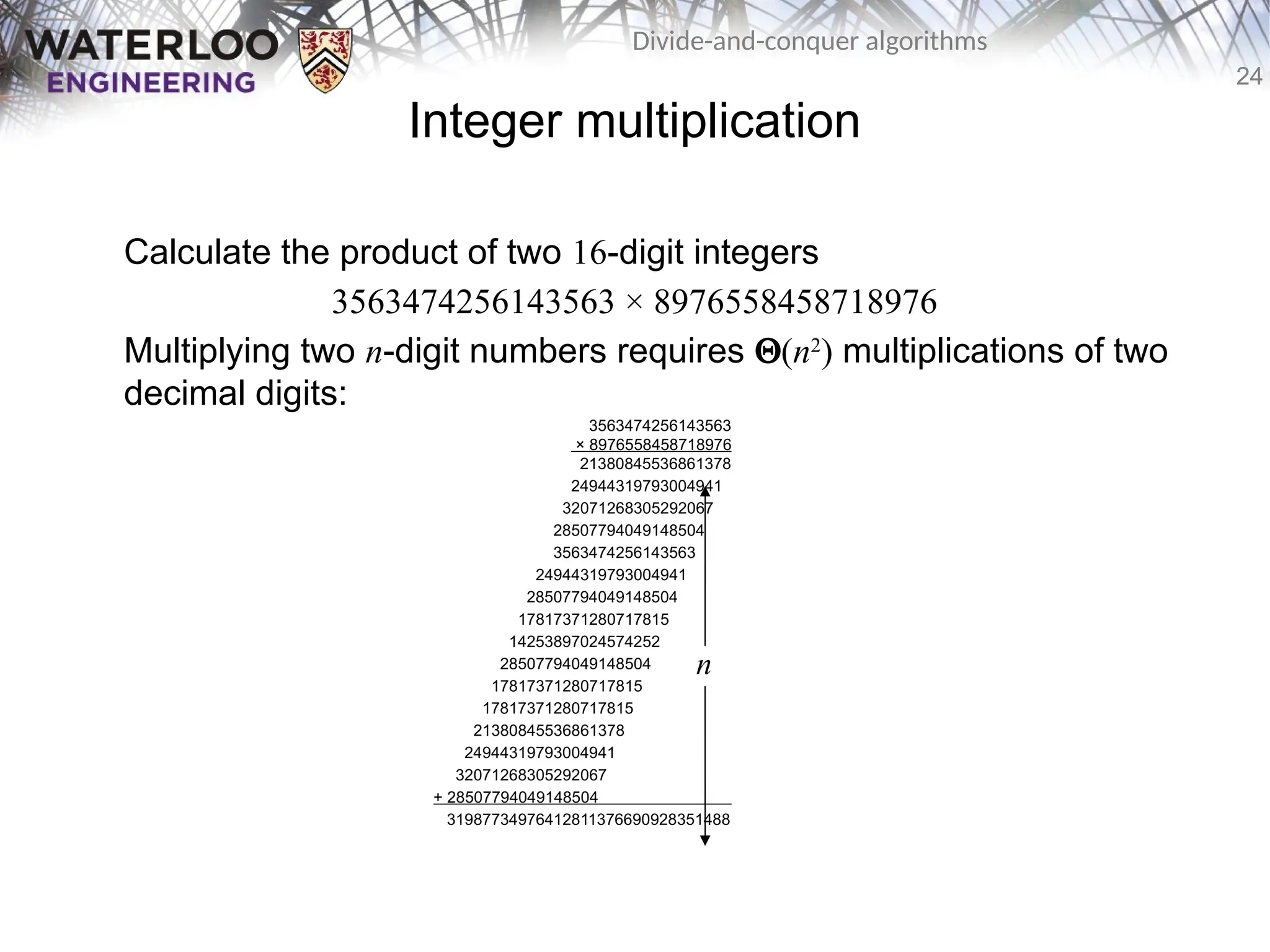
Calculatethe product of two 16-digit integers
3563474256143563 × 8976558458718976
Multiplying two n-digit numbers requires Q(n2
) multiplications of two
decimal digits:
3563474256143563
× 8976558458718976
21380845536861378
24944319793004941
32071268305292067
28507794049148504
3563474256143563
24944319793004941
28507794049148504
17817371280717815
14253897024574252
28507794049148504
17817371280717815
17817371280717815
21380845536861378
24944319793004941
32071268305292067
+ 28507794049148504 .
31987734976412811376690928351488
n
25.
25
Divide-and-conquer algorithms
Integer multiplication
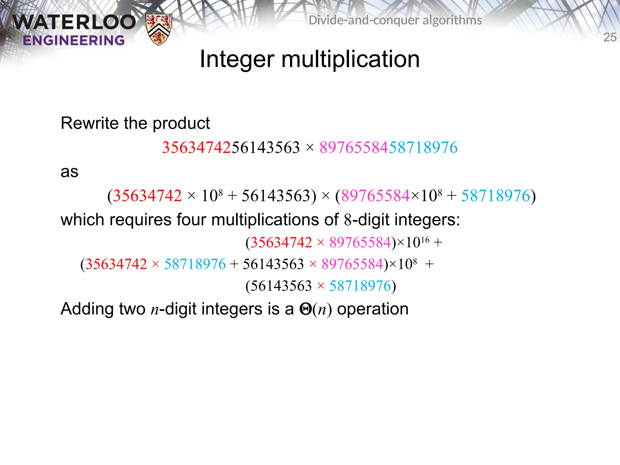
Rewritethe product
3563474256143563 × 8976558458718976
as
(35634742 × 108
+ 56143563) × (89765584×108
+ 58718976)
which requires four multiplications of 8-digit integers:
(35634742 × 89765584)×1016
+
(35634742 × 58718976 + 56143563 × 89765584)×108
+
(56143563 × 58718976)
Adding two n-digit integers is a Q(n) operation
26.
26
Divide-and-conquer algorithms
Integer multiplication
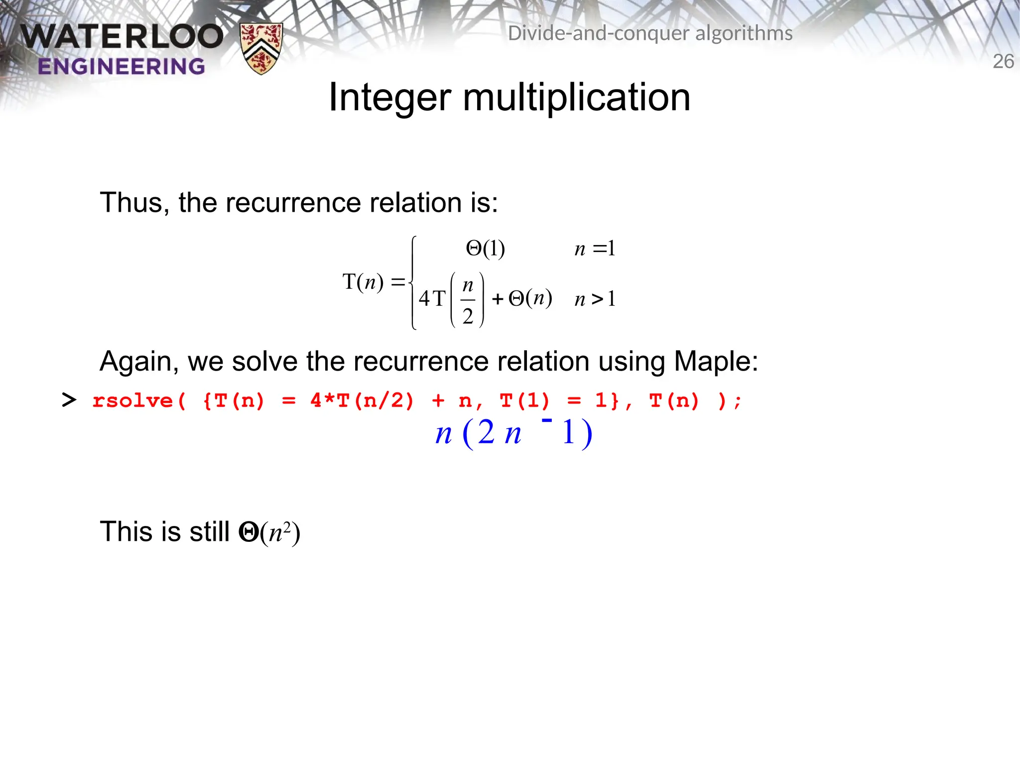
Thus,the recurrence relation is:
Again, we solve the recurrence relation using Maple:
> rsolve( {T(n) = 4*T(n/2) + n, T(1) = 1}, T(n) );
This is still Q(n2
)
(1) 1
T( )
( )
4T 1
2
n
n n
n n
n ( )
2 n 1
27.
27
Divide-and-conquer algorithms
Integer multiplication
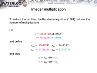
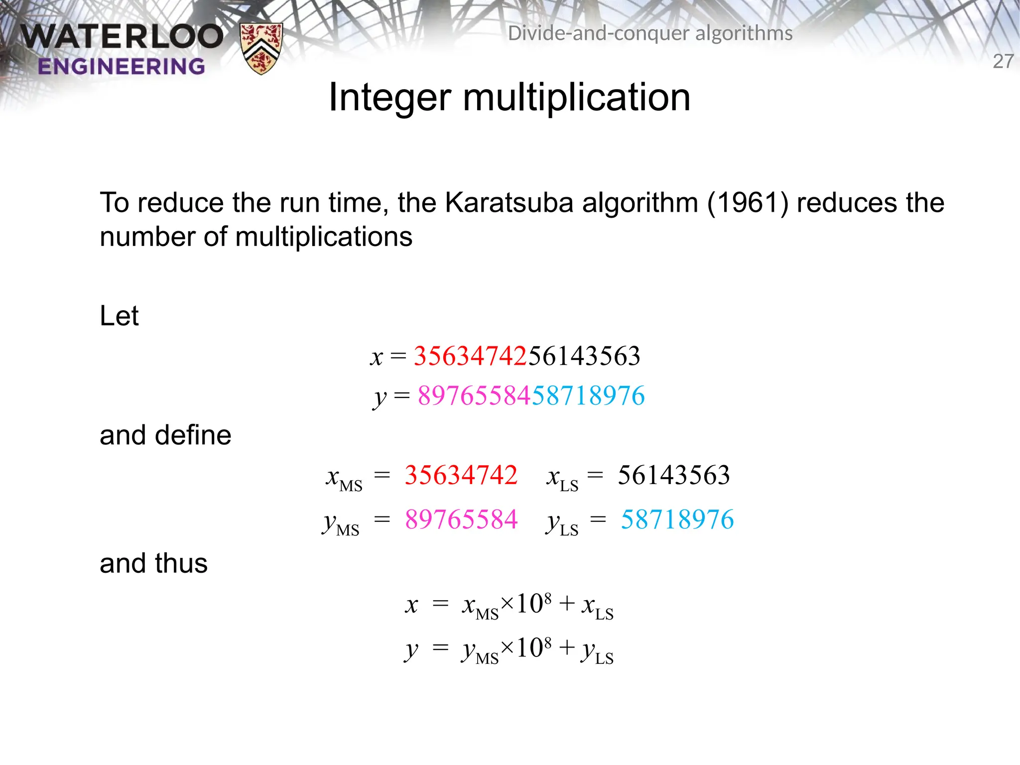
Toreduce the run time, the Karatsuba algorithm (1961) reduces the
number of multiplications
Let
x = 3563474256143563
y = 8976558458718976
and define
xMS = 35634742 xLS = 56143563
yMS = 89765584 yLS = 58718976
and thus
x = xMS×108
+ xLS
y = yMS×108
+ yLS
28.
28
Divide-and-conquer algorithms
Integer multiplication
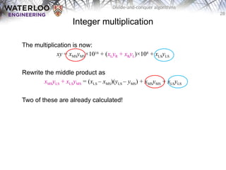
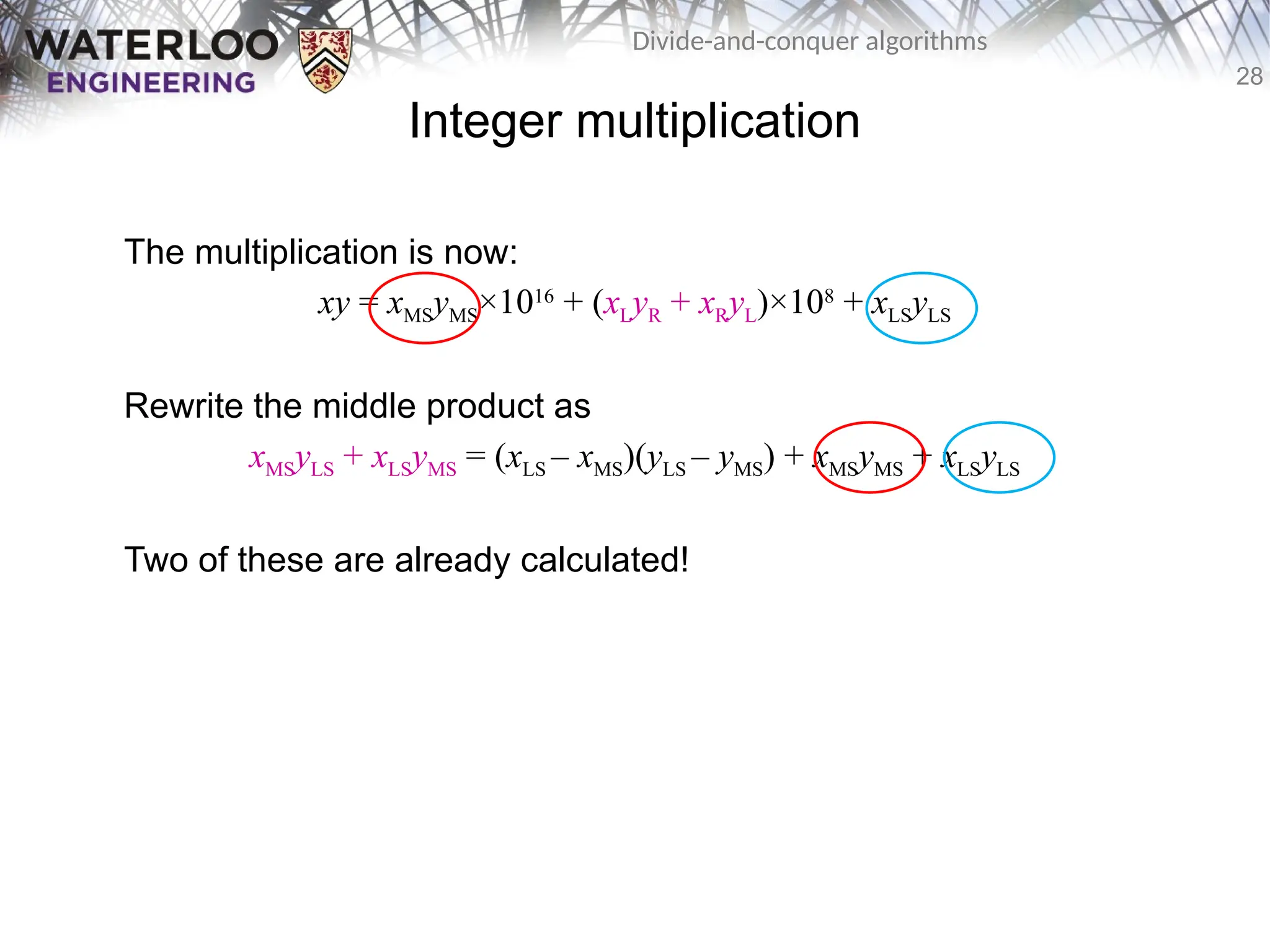
Themultiplication is now:
xy = xMSyMS×1016
+ (xLyR + xRyL)×108
+ xLSyLS
Rewrite the middle product as
xMSyLS + xLSyMS = (xLS – xMS)(yLS – yMS) + xMSyMS + xLSyLS
Two of these are already calculated!
29.
29
Divide-and-conquer algorithms
Integer multiplication
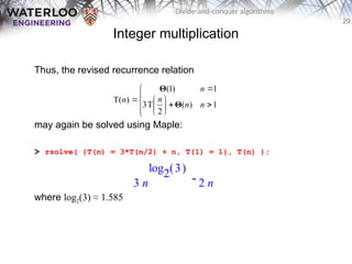
Thus,the revised recurrence relation
may again be solved using Maple:
> rsolve( {T(n) = 3*T(n/2) + n, T(1) = 1}, T(n) );
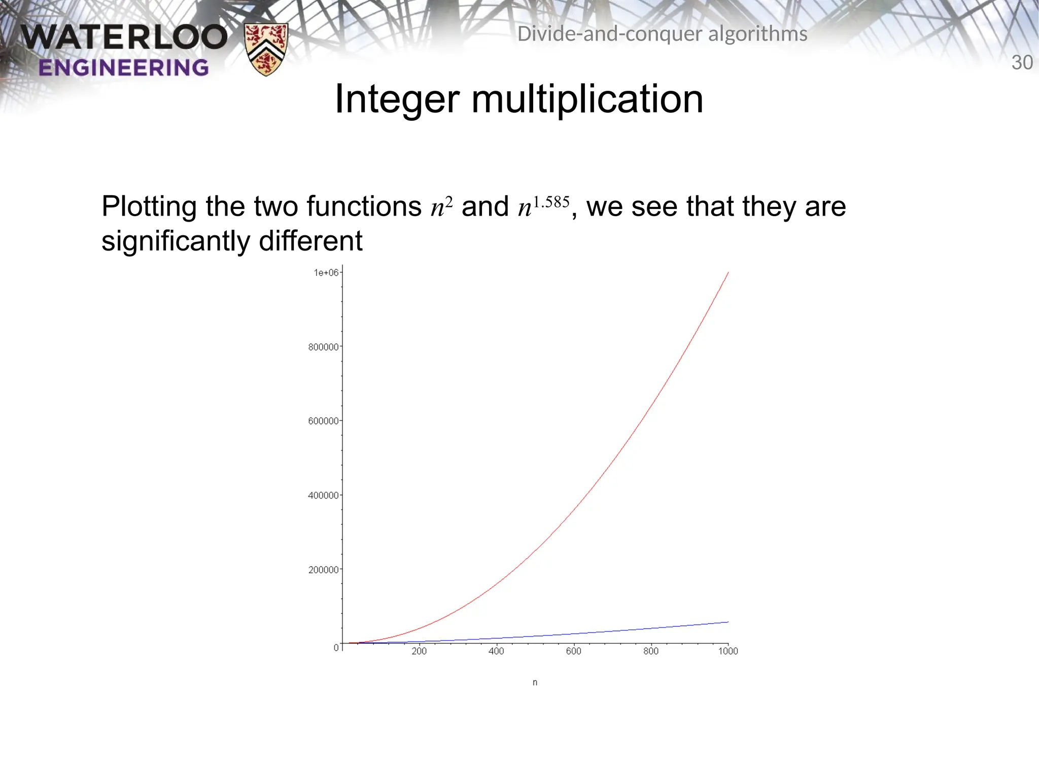
where log2(3) ≈ 1.585
1
)
(
2
T
3
1
)
1
(
)
T(
n
n
n
n
n
Θ
Θ
3 n
( )
log2 3
2 n
31
Divide-and-conquer algorithms
Integer multiplication
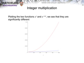
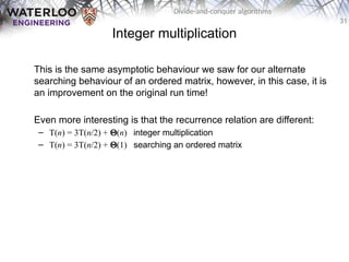
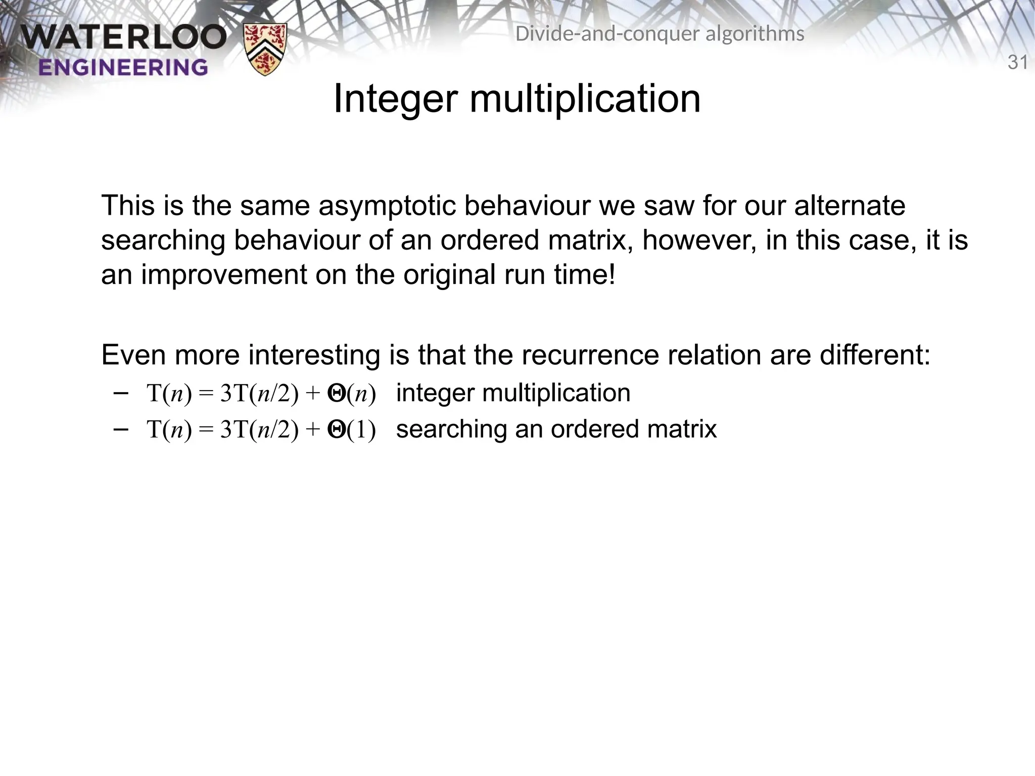
Thisis the same asymptotic behaviour we saw for our alternate
searching behaviour of an ordered matrix, however, in this case, it is
an improvement on the original run time!
Even more interesting is that the recurrence relation are different:
– T(n) = 3T(n/2) + Q(n) integer multiplication
– T(n) = 3T(n/2) + Q(1) searching an ordered matrix
32.
32
Divide-and-conquer algorithms
Integer multiplication
Inreality, you would probably not use this technique: there are
others
There are also libraries available for fast integer multiplication
For example, the GNU Image Manipulation Program (GIMP) comes
with a complete set of tools for fast integer arithmetic
http://www.gimp.org/
33.
33
Divide-and-conquer algorithms
Integer multiplication
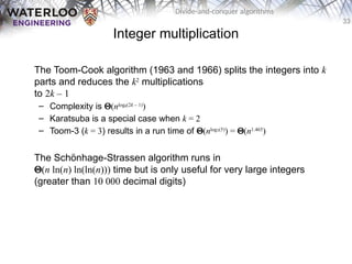
TheToom-Cook algorithm (1963 and 1966) splits the integers into k
parts and reduces the k2
multiplications
to 2k – 1
– Complexity is Q(nlogk(2k – 1)
)
– Karatsuba is a special case when k = 2
– Toom-3 (k = 3) results in a run time of Q(nlog3(5)
) = Q(n1.465
)
The Schönhage-Strassen algorithm runs in
Q(n ln(n) ln(ln(n))) time but is only useful for very large integers
(greater than 10 000 decimal digits)
34.
34
Divide-and-conquer algorithms
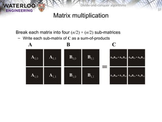
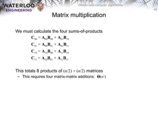
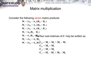
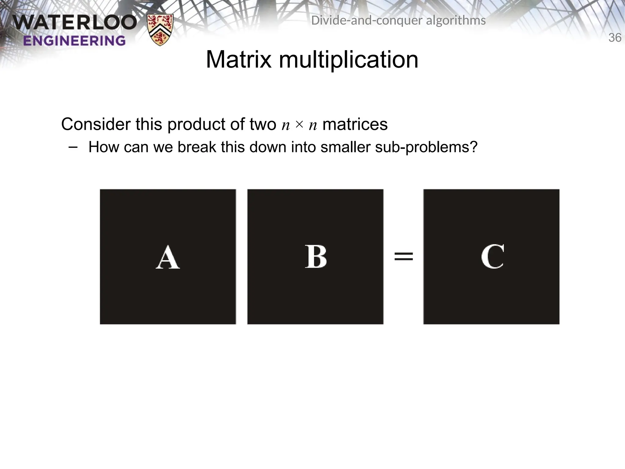
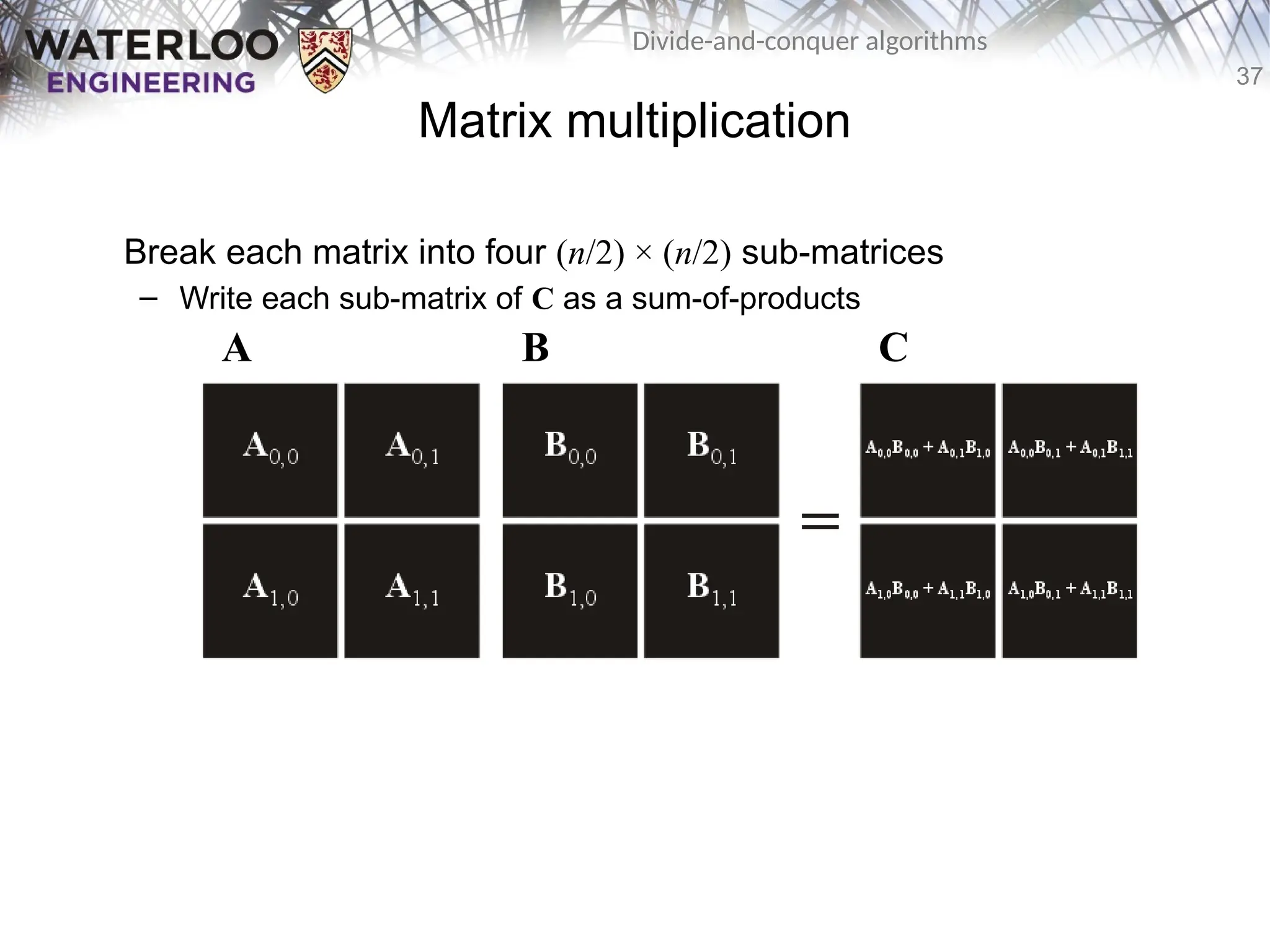
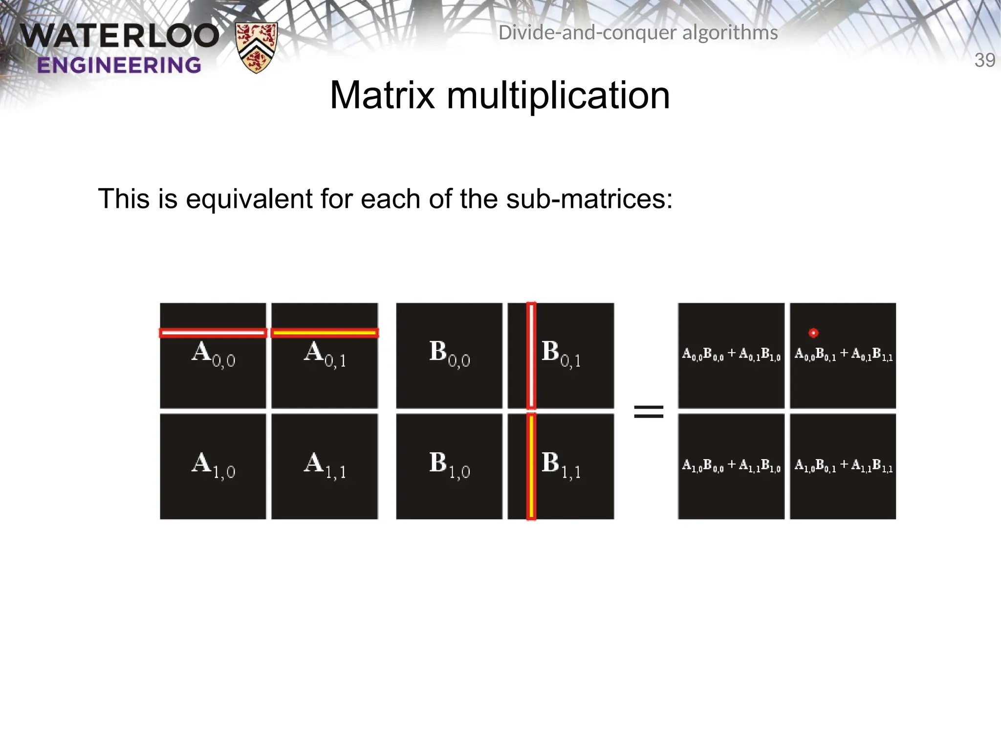
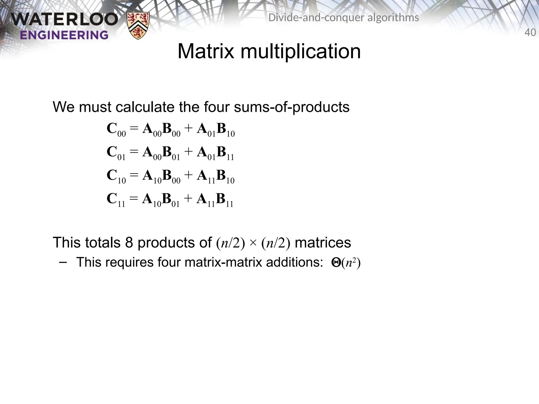
Matrix multiplication
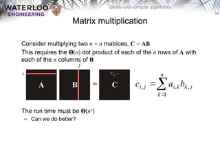
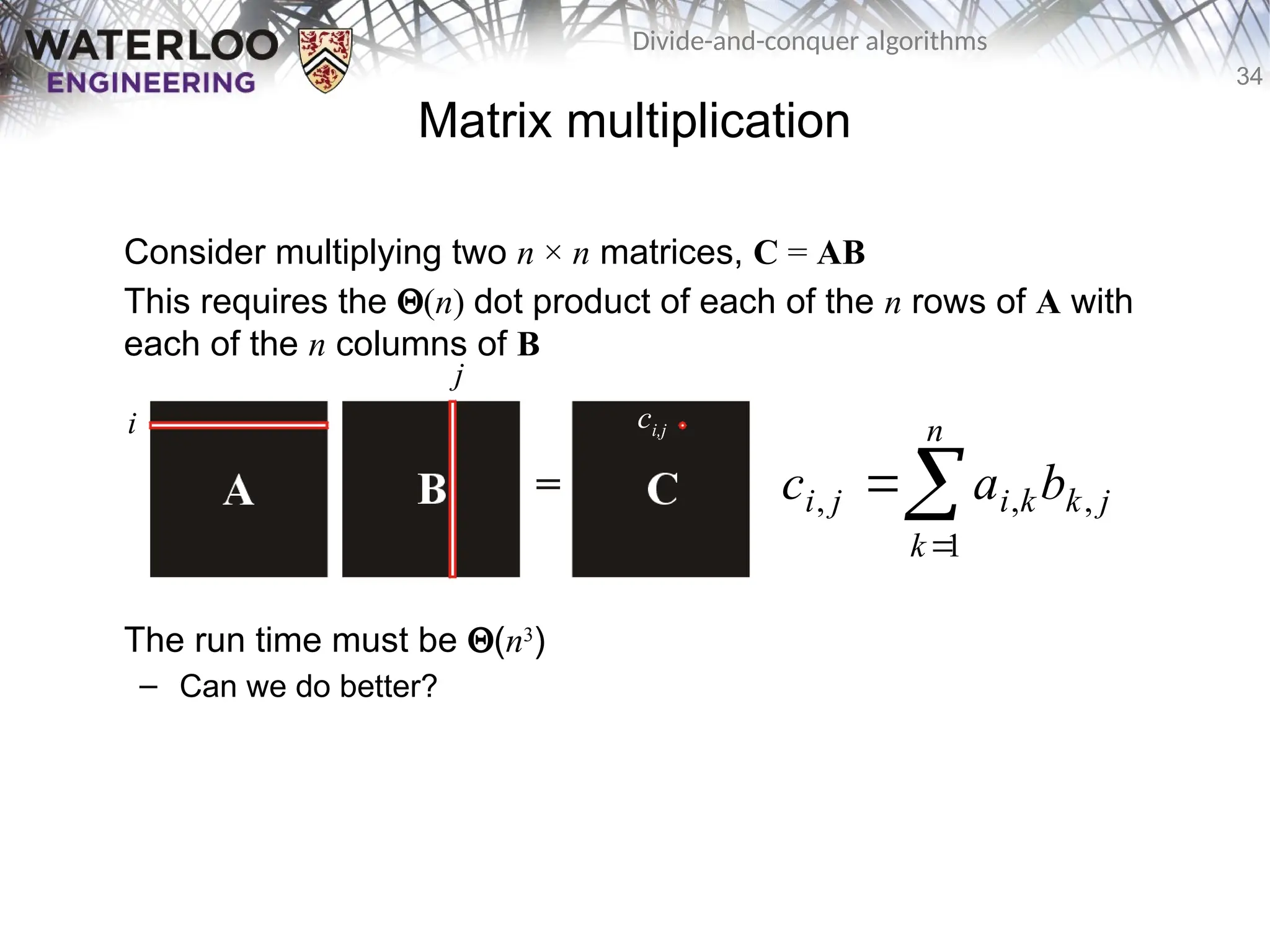
Considermultiplying two n × n matrices, C = AB
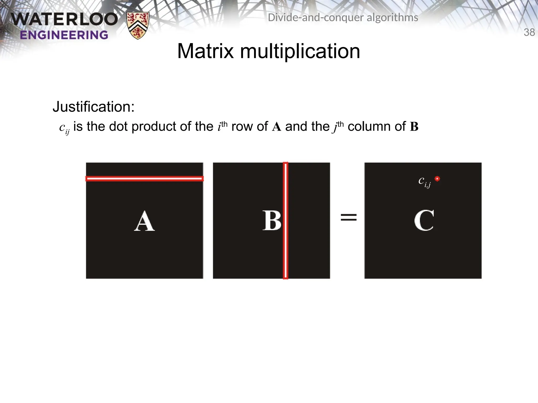
This requires the Q(n) dot product of each of the n rows of A with
each of the n columns of B
The run time must be Q(n3
)
– Can we do better?
n
k
j
k
k
i
j
i b
a
c
1
,
,
,
i
j
ci,j
35.
35
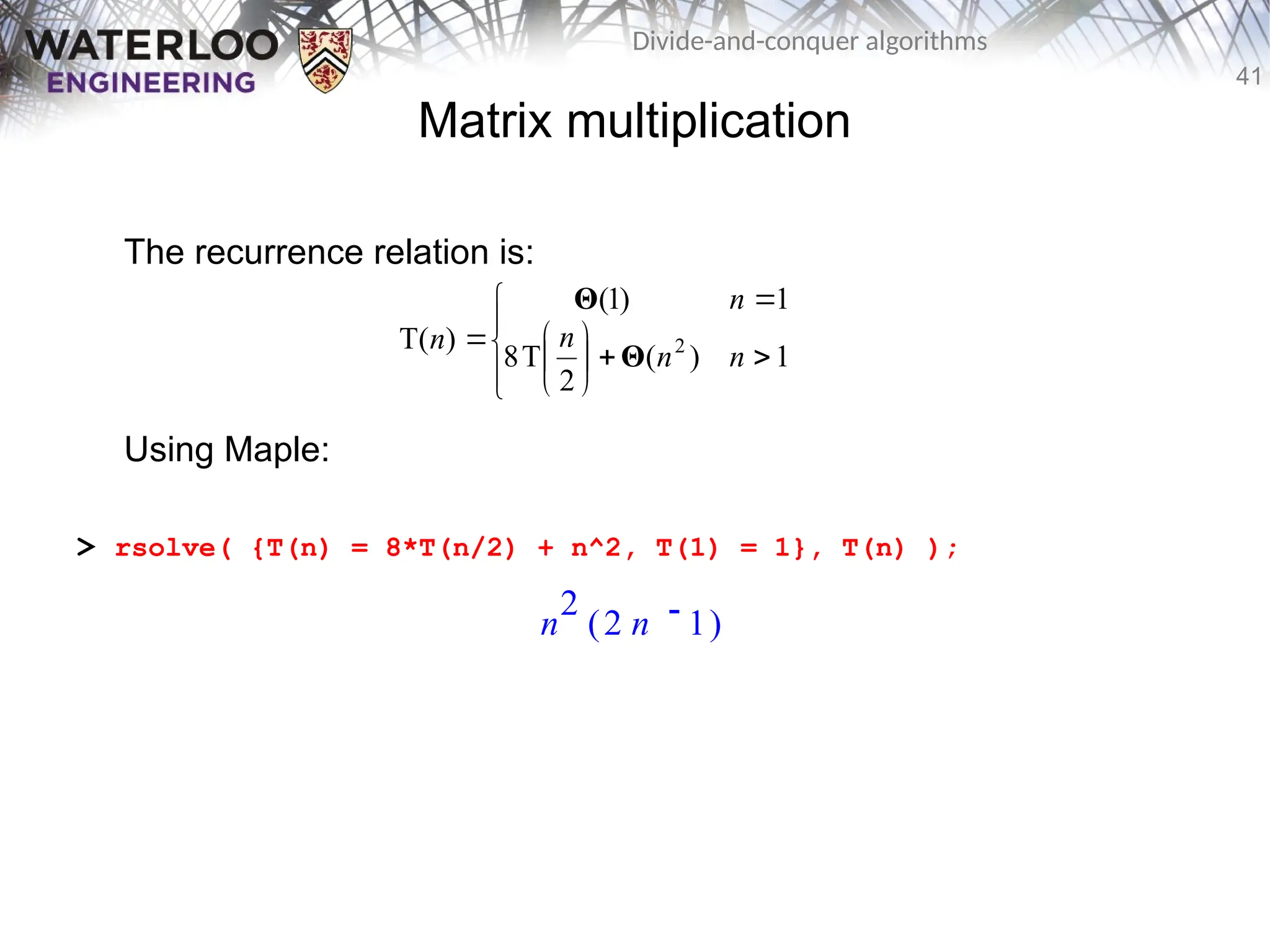
Divide-and-conquer algorithms
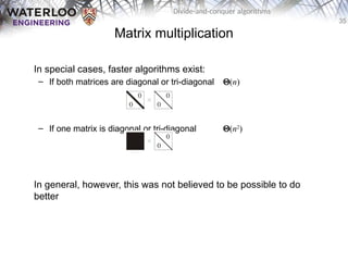
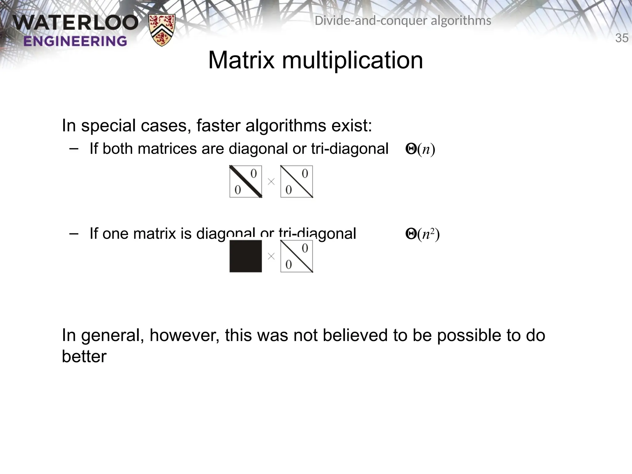
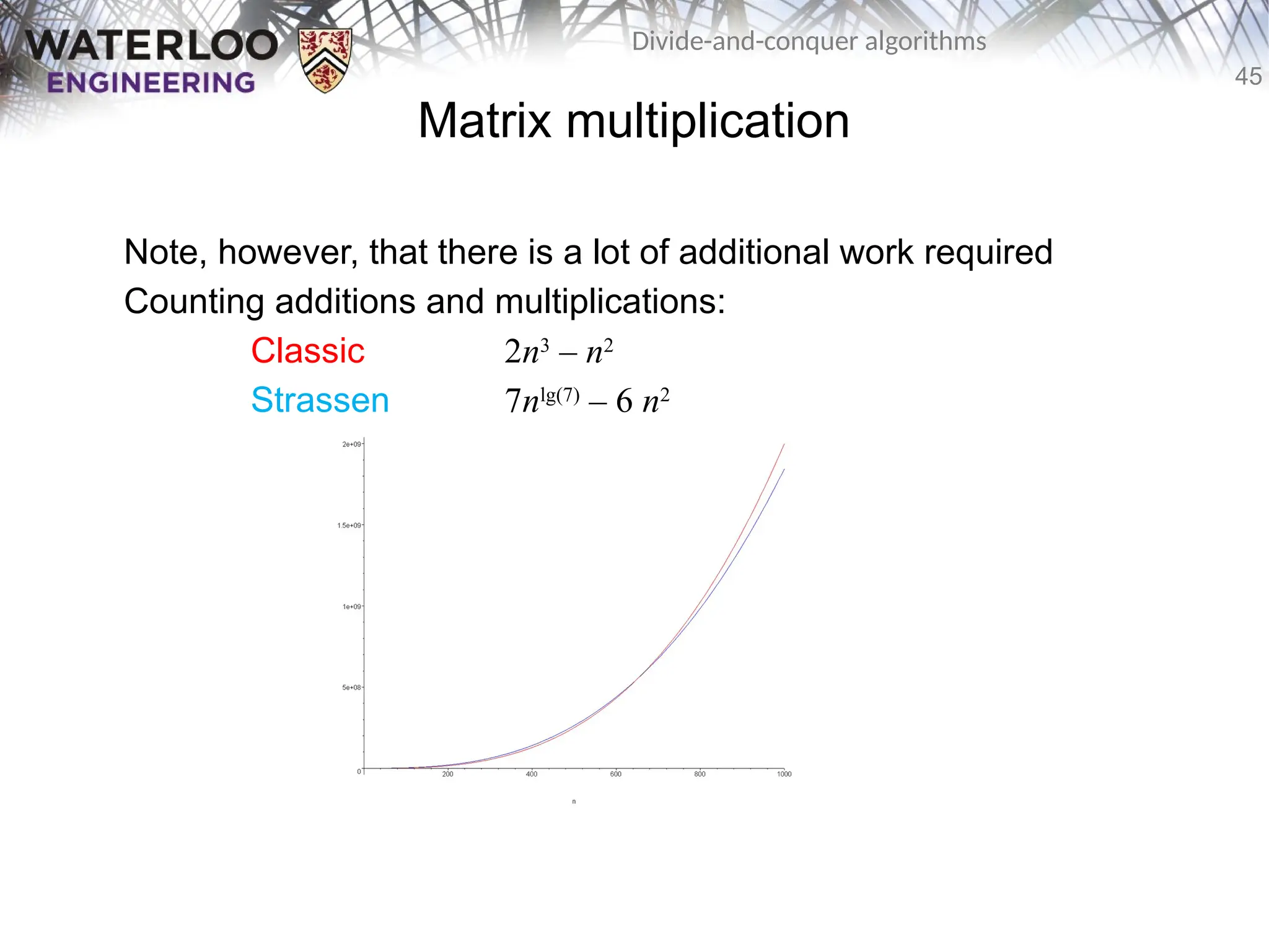
In specialcases, faster algorithms exist:
– If both matrices are diagonal or tri-diagonal Q(n)
– If one matrix is diagonal or tri-diagonal Q(n2
)
In general, however, this was not believed to be possible to do
better
Matrix multiplication
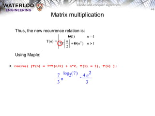
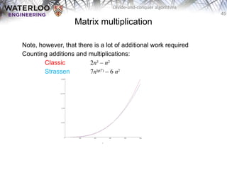
46
Divide-and-conquer algorithms
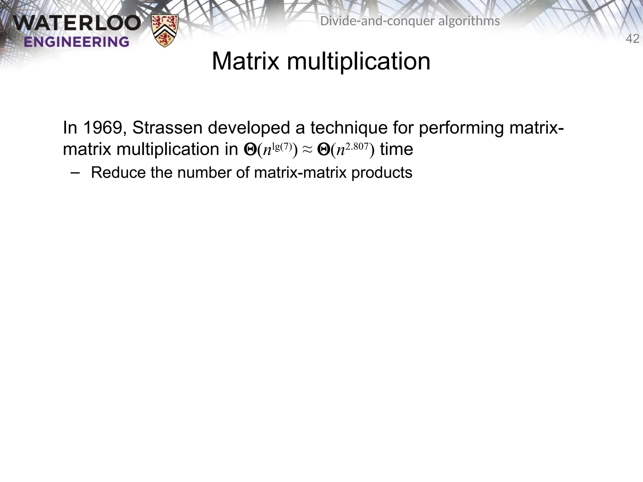
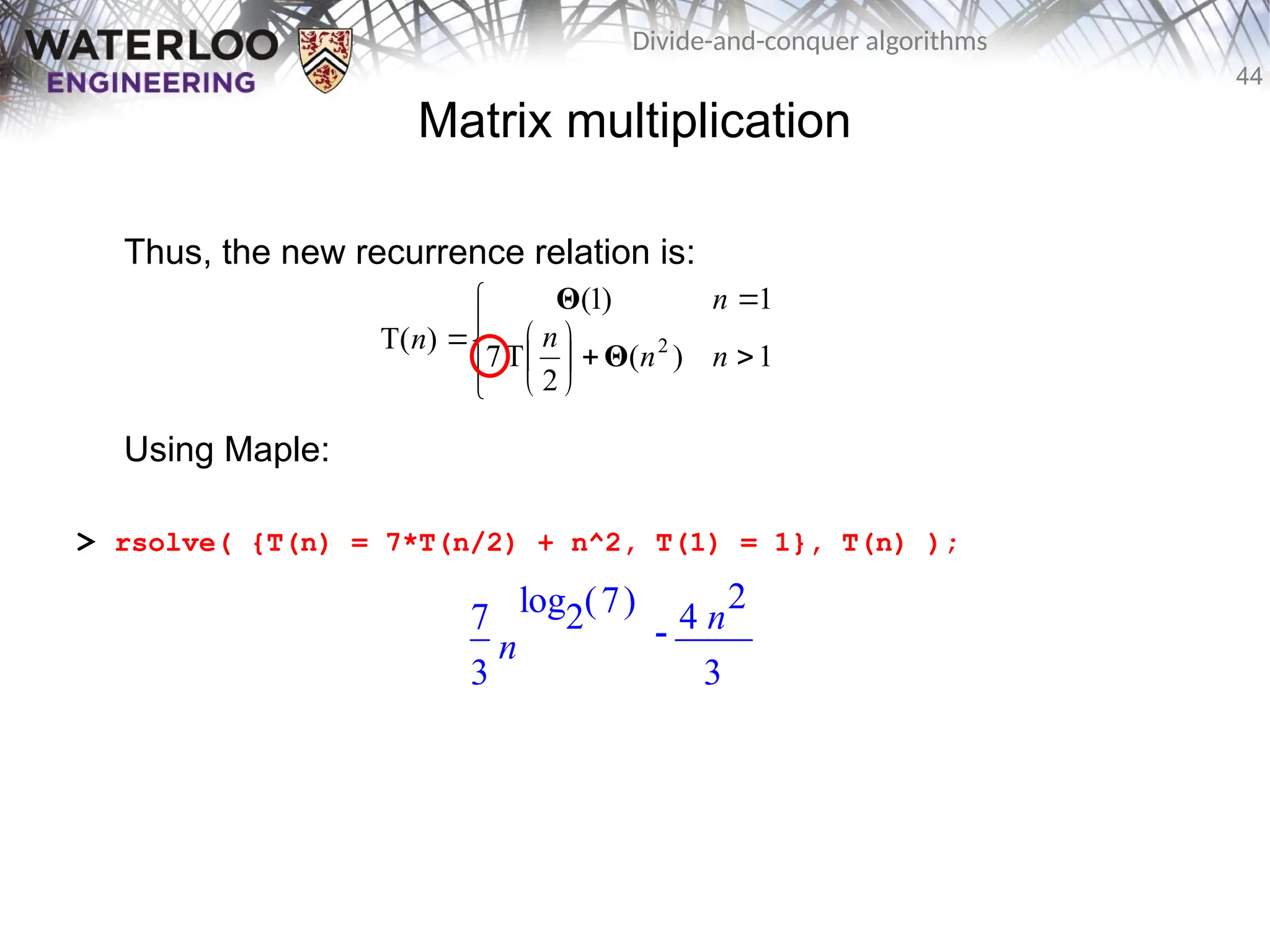
Matrix multiplication
Examiningthis plot, and then solving explicitly, we find that
Strassen’s method only reduces the number of operations for n >
654
– Better asymptotic behaviour does not immediately translate into better
run-times
The Strassen algorithm is not the fastest
– the Coppersmith–Winograd algorithm runs in Q(n2.376
) time but the
coefficients are too large for any problem
Therefore, better asymptotic behaviour does not immediately
translate into better run-times
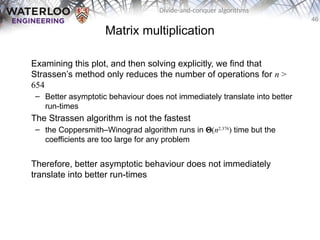
48
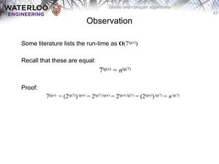
Divide-and-conquer algorithms
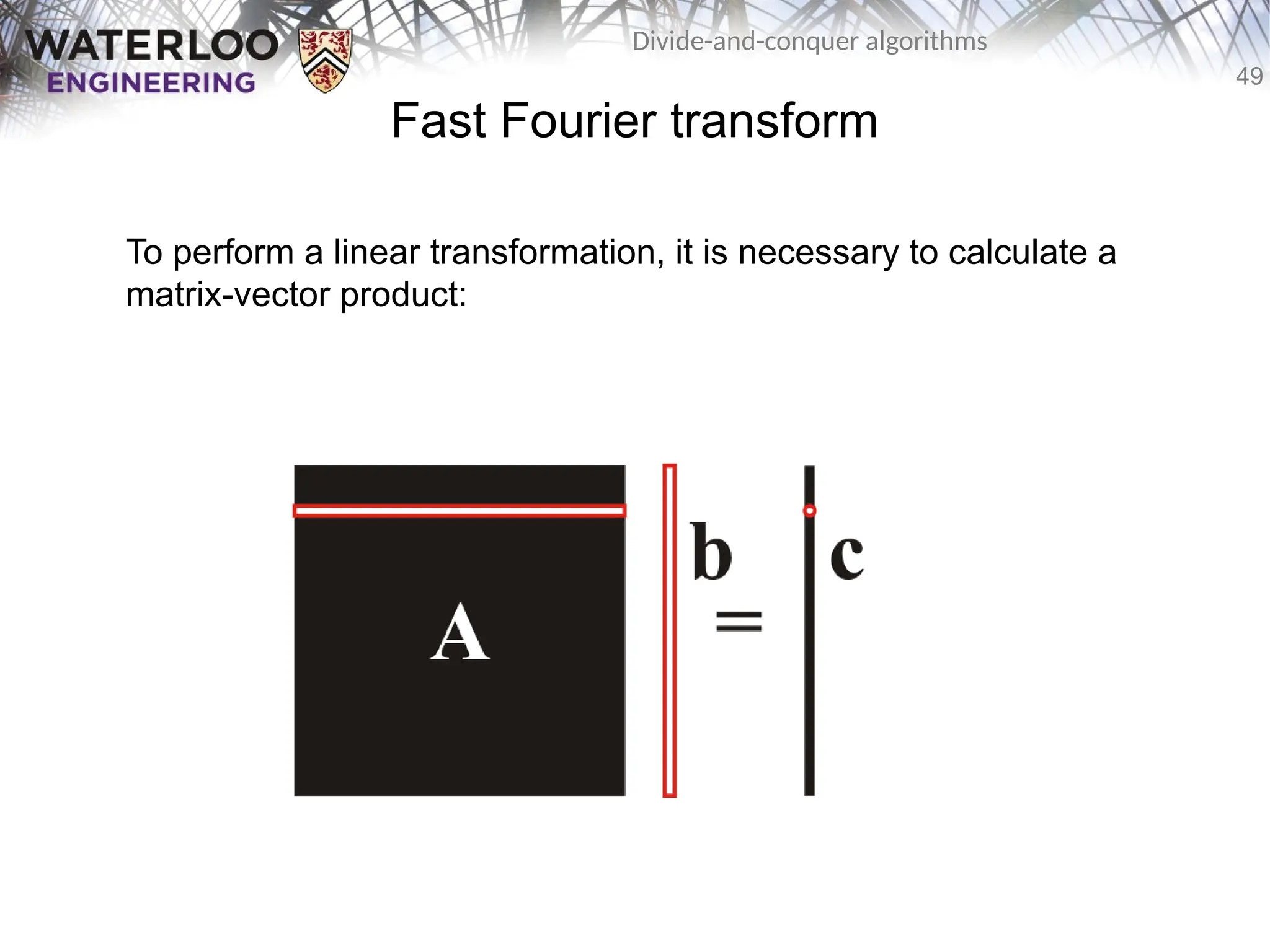
Fast Fouriertransform
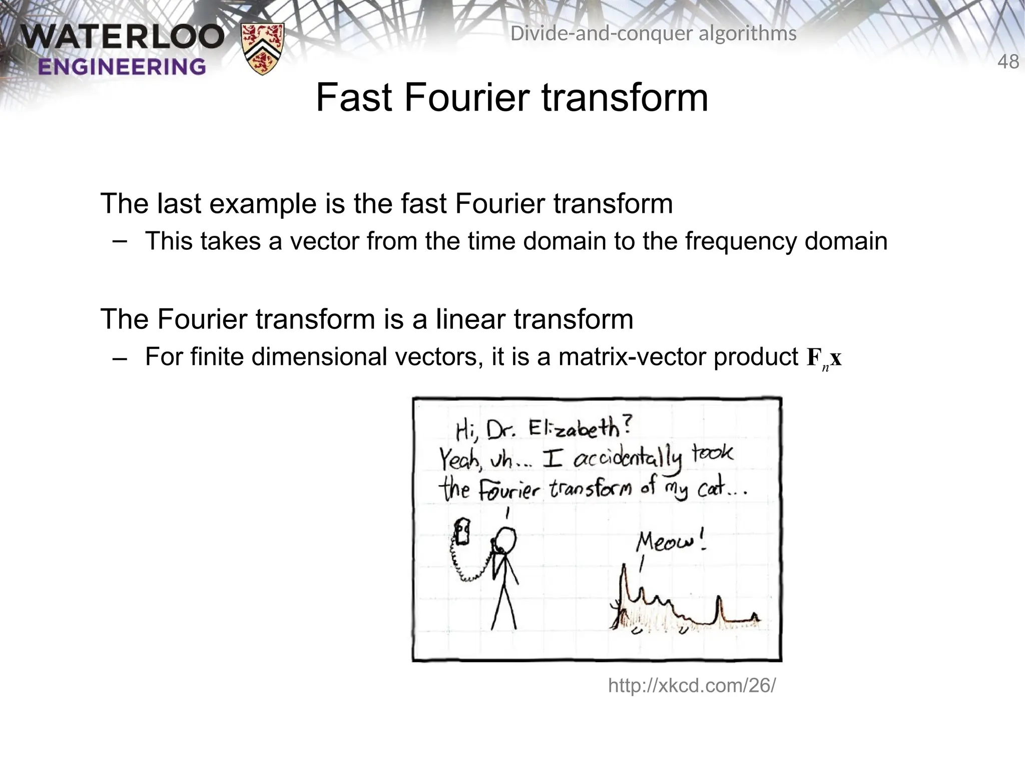
The last example is the fast Fourier transform
– This takes a vector from the time domain to the frequency domain
The Fourier transform is a linear transform
– For finite dimensional vectors, it is a matrix-vector product Fnx
http://xkcd.com/26/
50
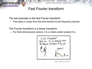
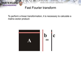
Divide-and-conquer algorithms
Fast Fouriertransform
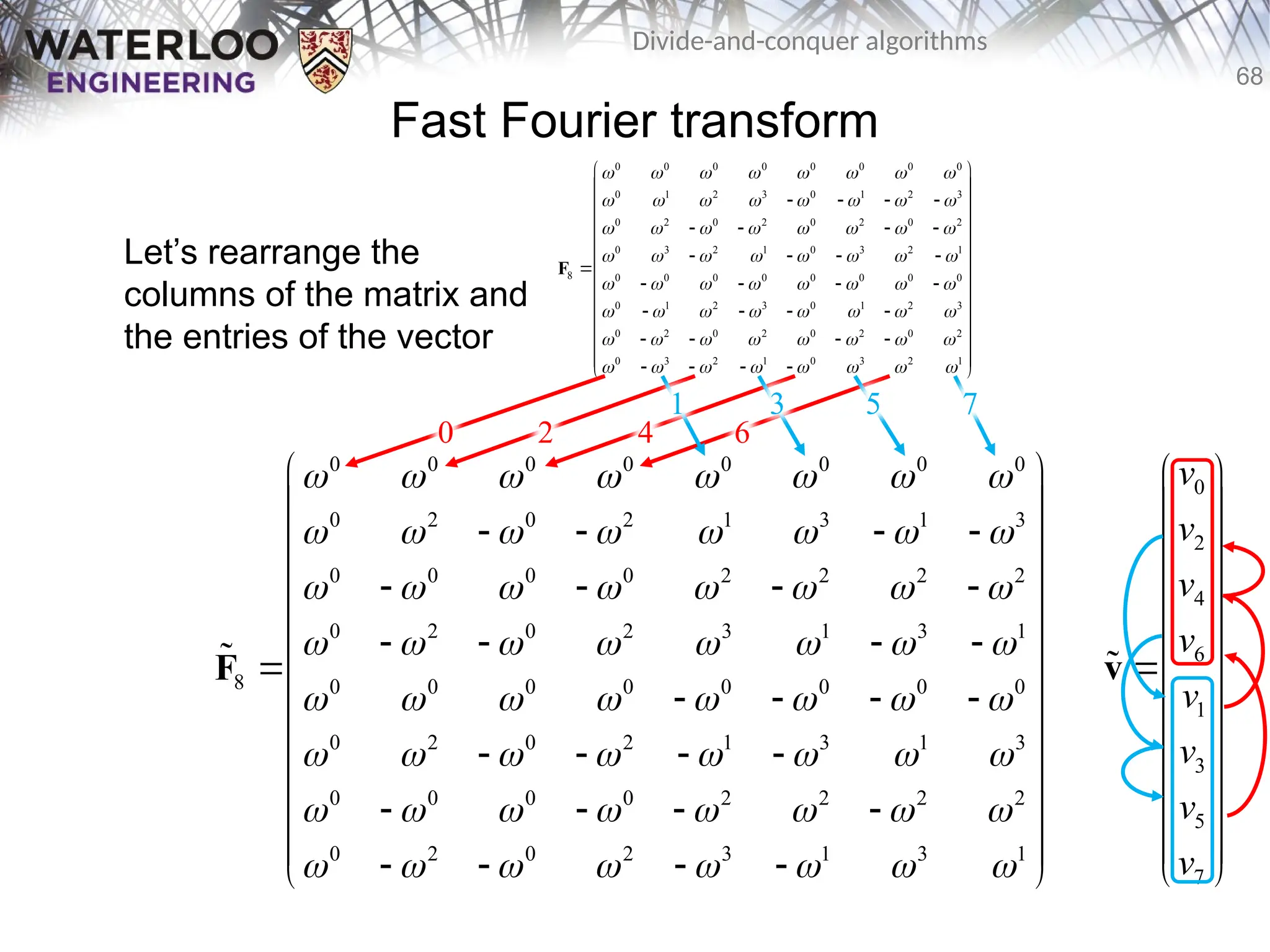
We can apply a divide and conquer algorithm to this problem
– Break the matrix-vector product into four matrix-vector products,
each of half the size
51.
51
Divide-and-conquer algorithms
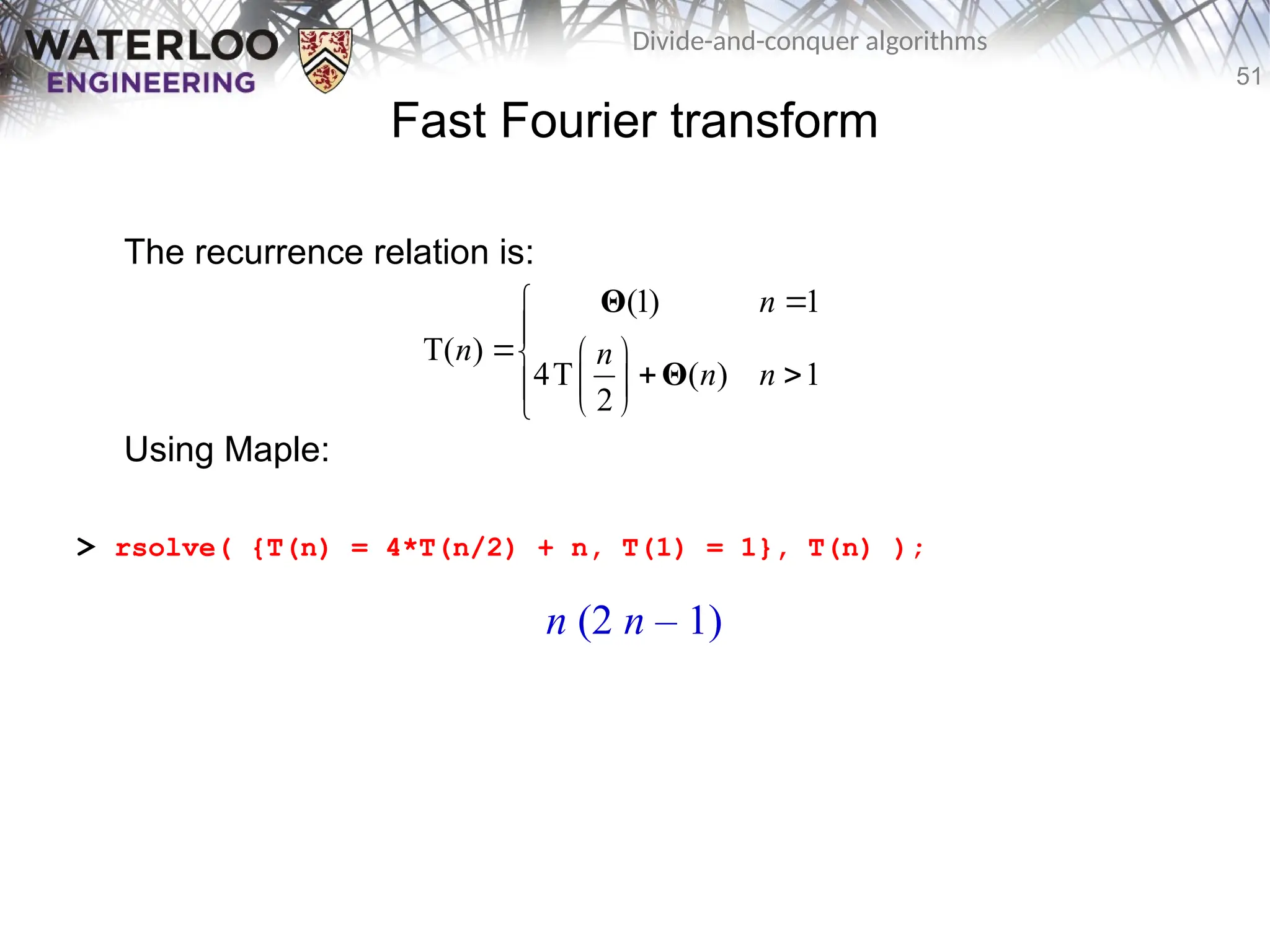
Fast Fouriertransform
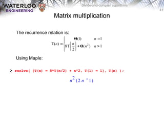
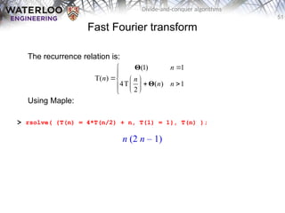
The recurrence relation is:
Using Maple:
> rsolve( {T(n) = 4*T(n/2) + n, T(1) = 1}, T(n) );
(1) 1
T( )
4T ( ) 1
2
n
n n
n n
Θ
Θ
n (2 n – 1)
52.
52
Divide-and-conquer algorithms
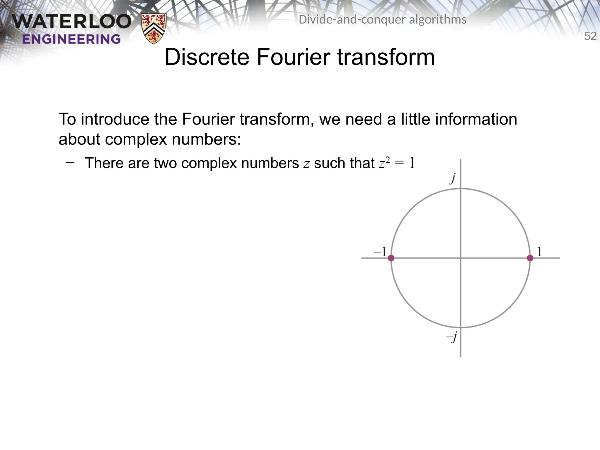
Discrete Fouriertransform
To introduce the Fourier transform, we need a little information
about complex numbers:
– There are two complex numbers z such that z2
= 1
53.
53
Divide-and-conquer algorithms
Discrete Fouriertransform
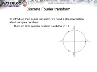
To introduce the Fourier transform, we need a little information
about complex numbers:
– There are three complex numbers z such that z3
= 1
54.
54
Divide-and-conquer algorithms
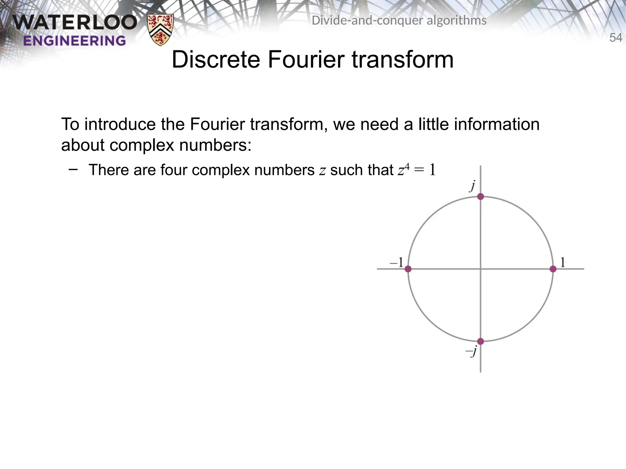
Discrete Fouriertransform
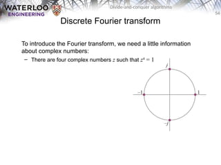
To introduce the Fourier transform, we need a little information
about complex numbers:
– There are four complex numbers z such that z4
= 1
55.
55
Divide-and-conquer algorithms
Discrete Fouriertransform
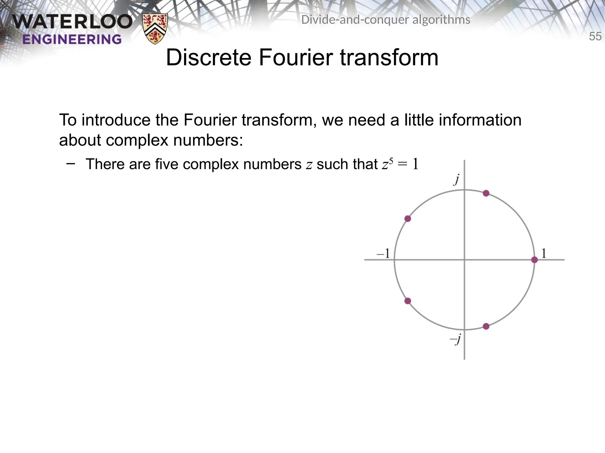
To introduce the Fourier transform, we need a little information
about complex numbers:
– There are five complex numbers z such that z5
= 1
56.
56
Divide-and-conquer algorithms
Discrete Fouriertransform
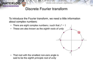
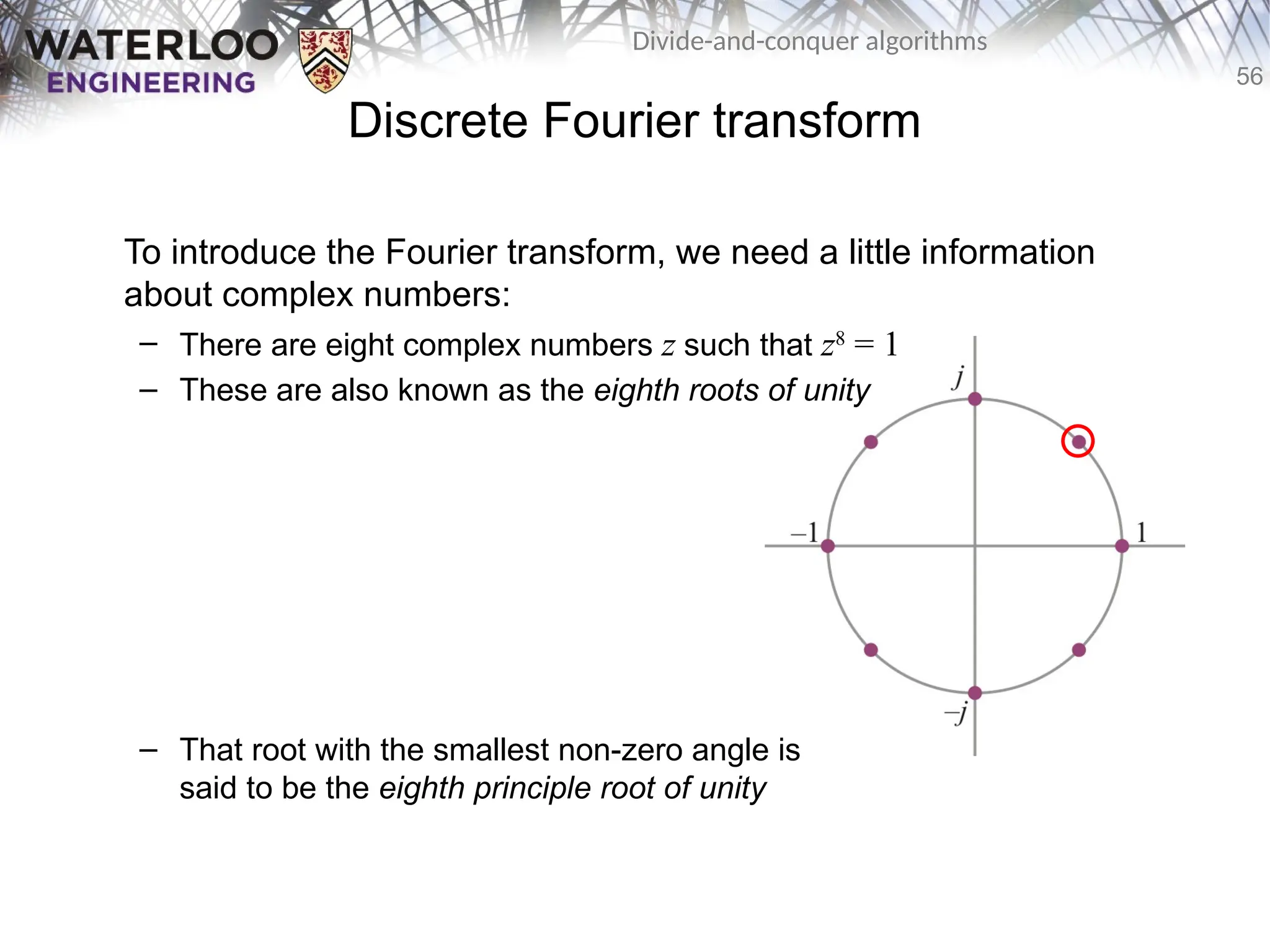
To introduce the Fourier transform, we need a little information
about complex numbers:
– There are eight complex numbers z such that z8
= 1
– These are also known as the eighth roots of unity
– That root with the smallest non-zero angle is
said to be the eighth principle root of unity
57.
57
Divide-and-conquer algorithms
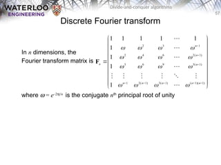
Discrete Fouriertransform
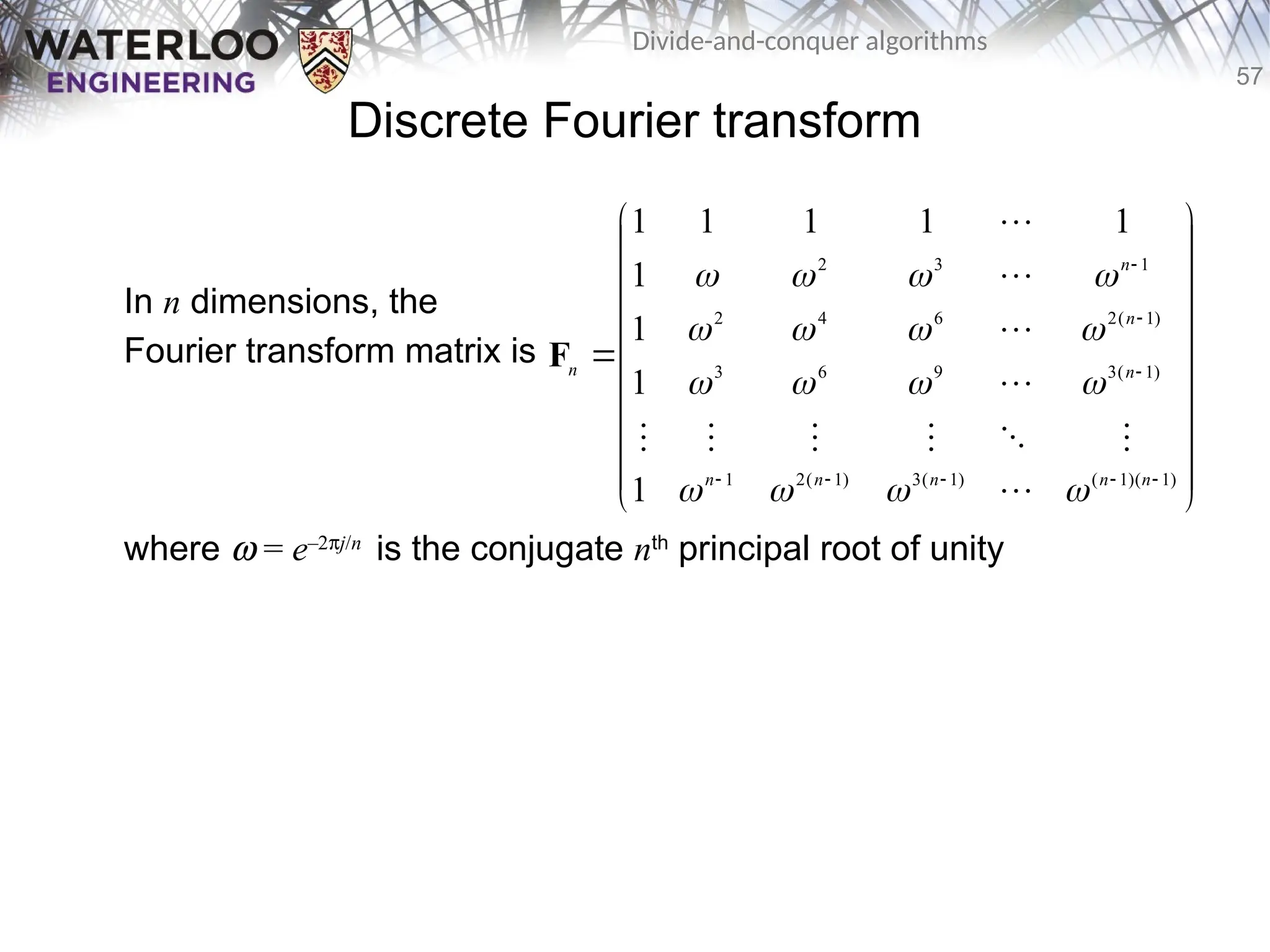
In n dimensions, the
Fourier transform matrix is
where w = e–2pj/n
is the conjugate nth
principal root of unity
)
1
)(
1
(
)
1
(
3
)
1
(
2
1
)
1
(
3
9
6
3
)
1
(
2
6
4
2
1
3
2
1
1
1
1
1
1
1
1
1
n
n
n
n
n
n
n
n
n
F
58.
58
Divide-and-conquer algorithms
Discrete Fouriertransform
For example, the matrix for the Fourier transform for 4-dimensions is
Here, w = –j is the conjugate 4th
principal root of unity
Note that:
– The matrix is symmetric
– All the column/row vectors are orthogonal
– These create a orthogonal basis for C4
4
1 1 1 1
1 1
1 1 1 1
1 1
j j
j j
F
59.
59
Divide-and-conquer algorithms
Discrete Fouriertransform
Any matrix-vector multiplication is usually Q(n2
)
– The discrete Fourier transform is a useful tool in all fields of engineering
– In general, it is not possible to speed up a matrix-vector multiplication
– In this case, however, the matrix has a peculiar shape
• That of a very special Vandermonde matrix
60.
60
Divide-and-conquer algorithms
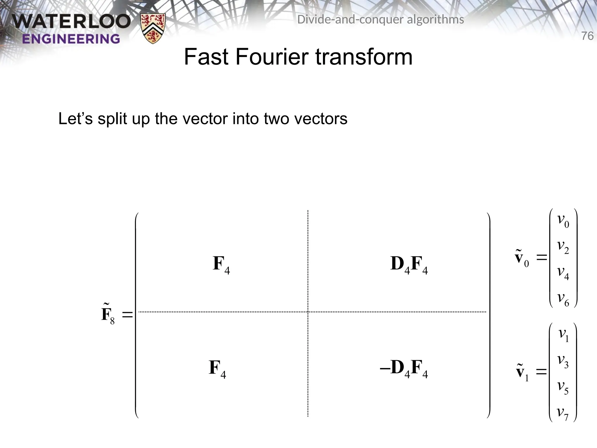
Fast Fouriertransform
We will now look at the Cooley–Tukey algorithm for calculating the
discrete Fourier transform
– This fast transform can only be applied the dimension is a power of two
– We will look at the 8-dimensional transform matrix
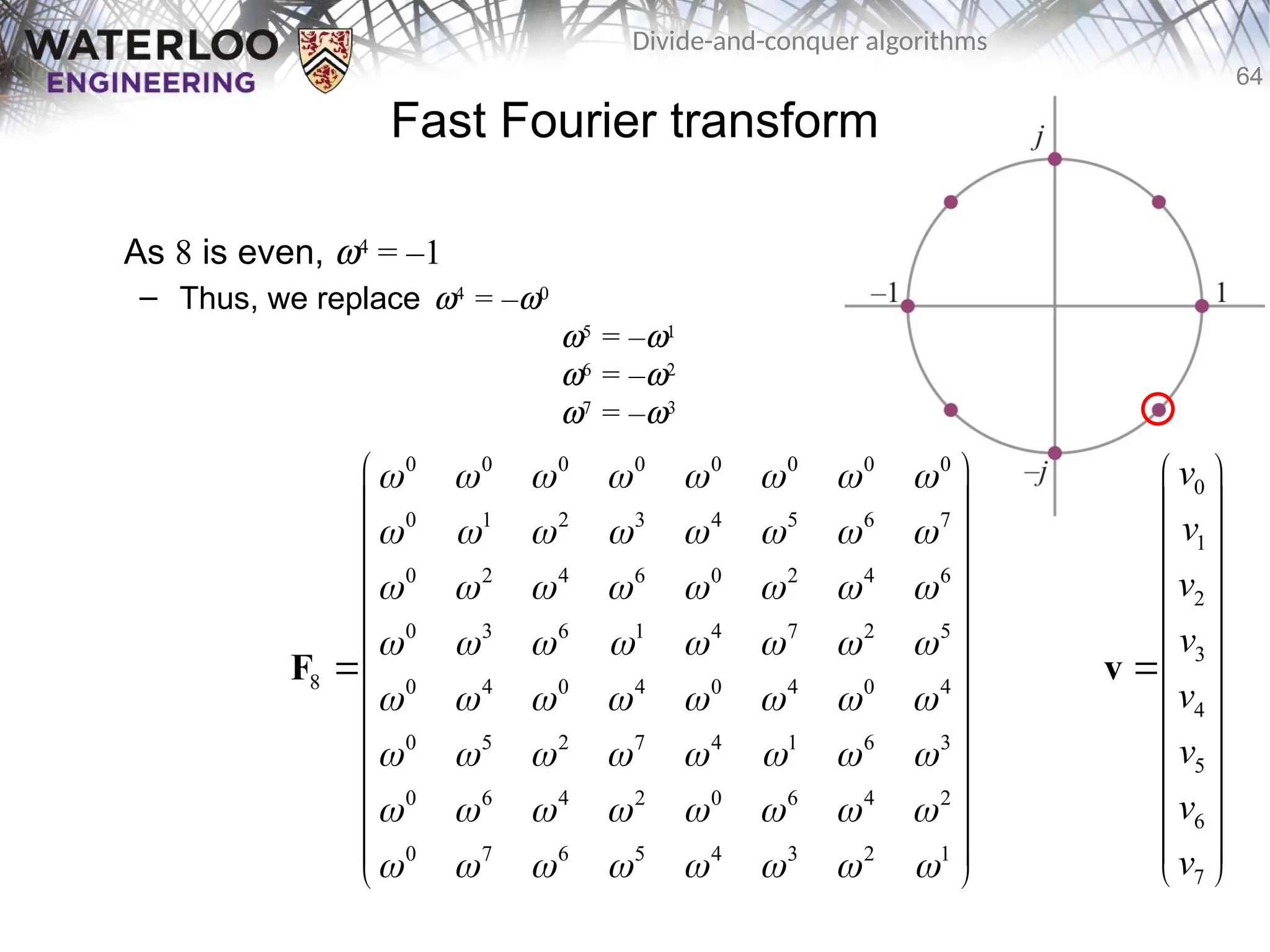
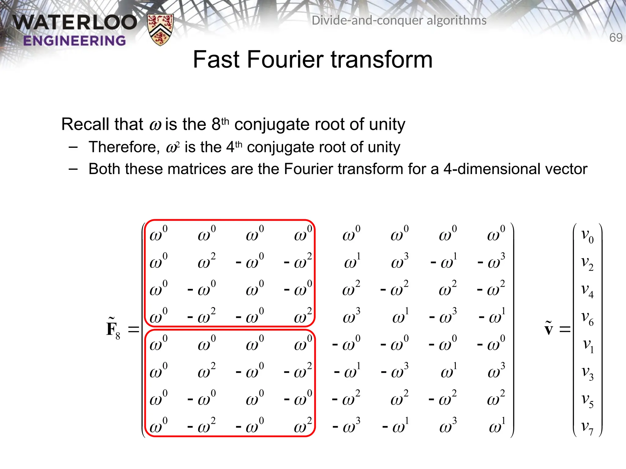
– The eighth conjugate root of unity is
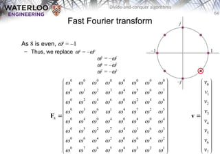
– Note that w2
= –j, w4
= –1 and w8
= 1
1 1
2 2
j
61.
61
Divide-and-conquer algorithms
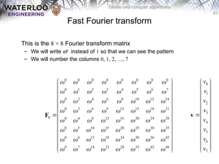
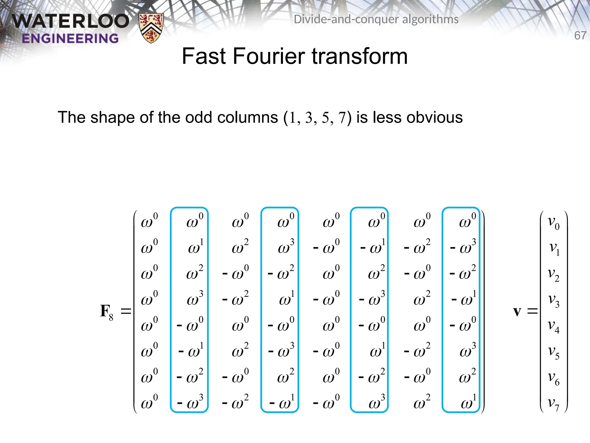
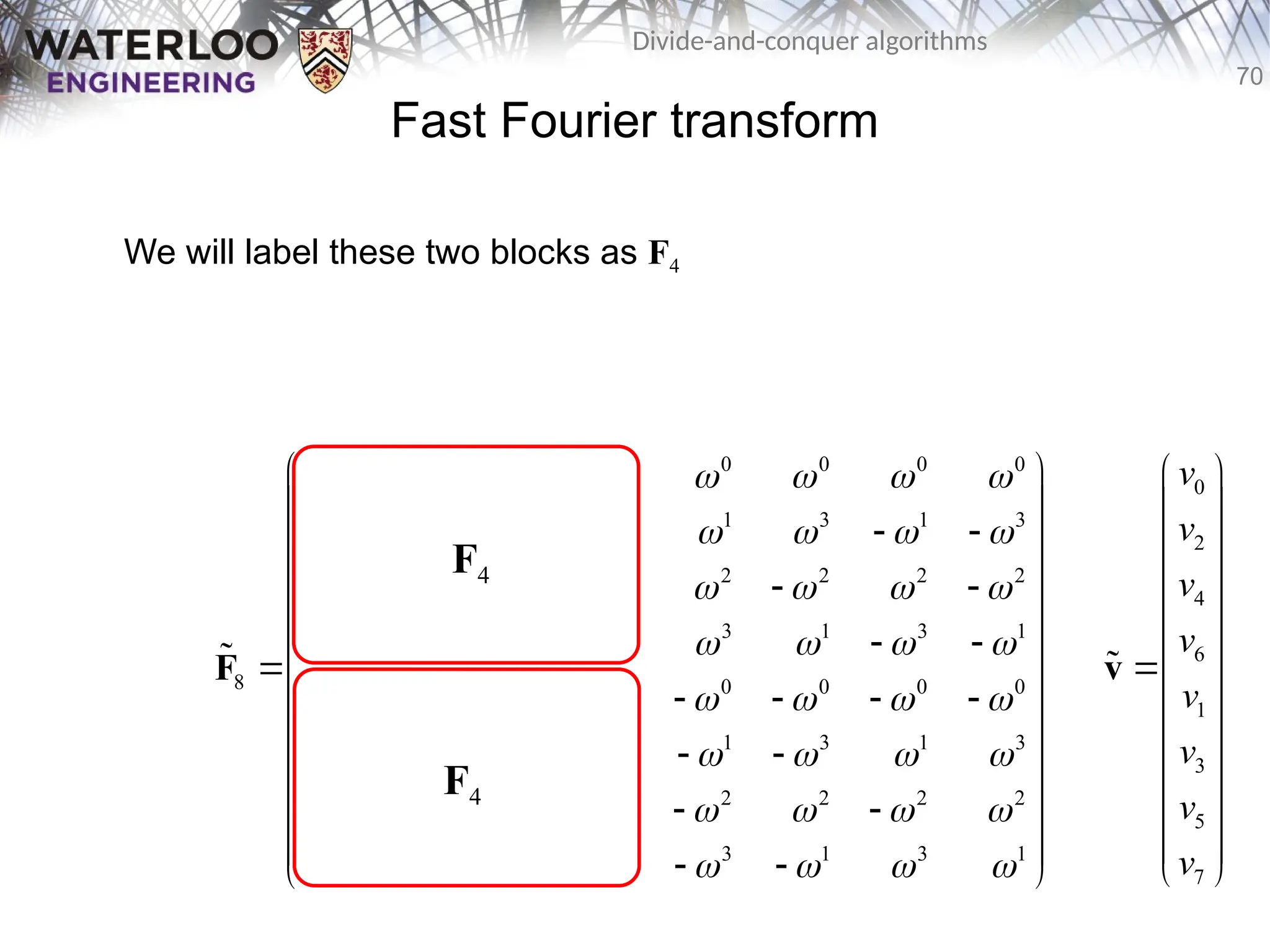
Fast Fouriertransform
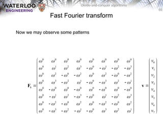
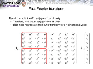
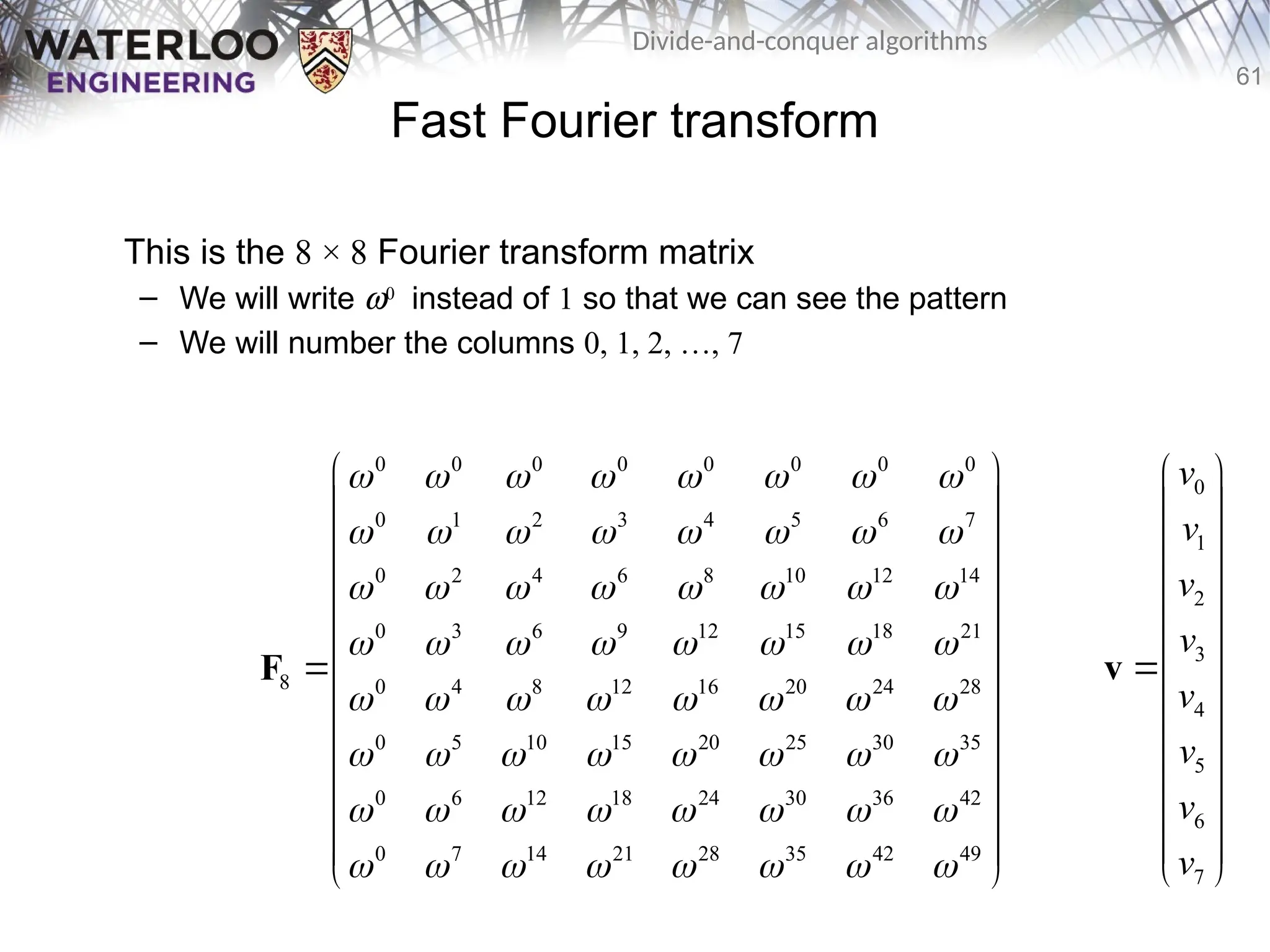
This is the 8 × 8 Fourier transform matrix
– We will write w0
instead of 1 so that we can see the pattern
– We will number the columns 0, 1, 2, …, 7
0 0 0 0 0 0 0 0
0 1 2 3 4 5 6 7
0 2 4 6 8 10 12 14
0 3 6 9 12 15 18 21
8 0 4 8 12 16 20 24 28
0 5 10 15 20 25 30 35
0 6 12 18 24 30 36 42
0 7 14 21 28 35 42 49
F
0
1
2
3
4
5
6
7
v
v
v
v
v
v
v
v
v
62.
62
Divide-and-conquer algorithms
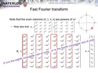
Fast Fouriertransform
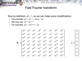
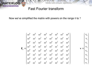
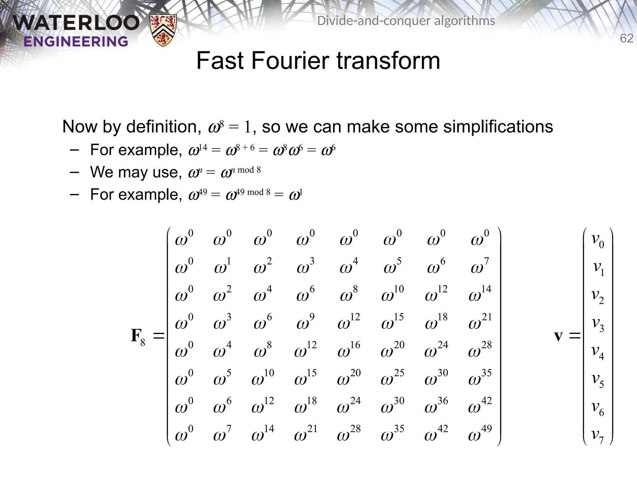
Now by definition, w8
= 1, so we can make some simplifications
– For example, w14
= w8 + 6
= w8
w6
= w6
– We may use, wn
= wn mod 8
– For example, w49
= w49 mod 8
= w1
0 0 0 0 0 0 0 0
0 1 2 3 4 5 6 7
0 2 4 6 8 10 12 14
0 3 6 9 12 15 18 21
8 0 4 8 12 16 20 24 28
0 5 10 15 20 25 30 35
0 6 12 18 24 30 36 42
0 7 14 21 28 35 42 49
F
0
1
2
3
4
5
6
7
v
v
v
v
v
v
v
v
v
77
Divide-and-conquer algorithms
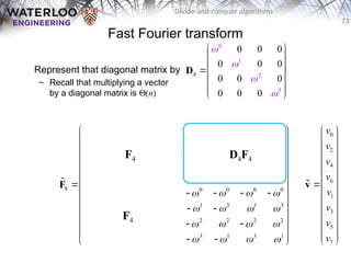
Fast Fouriertransform
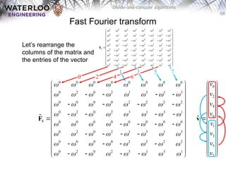
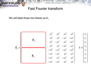
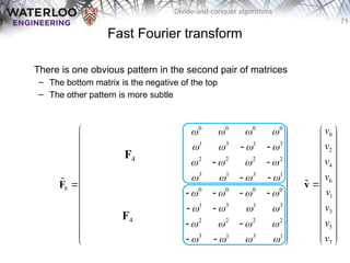
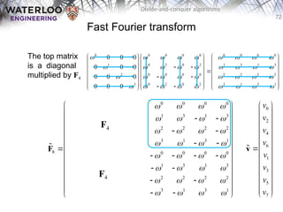
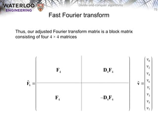
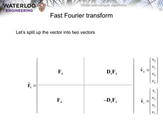
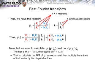
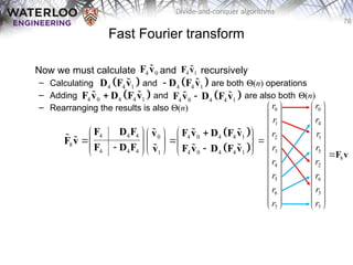
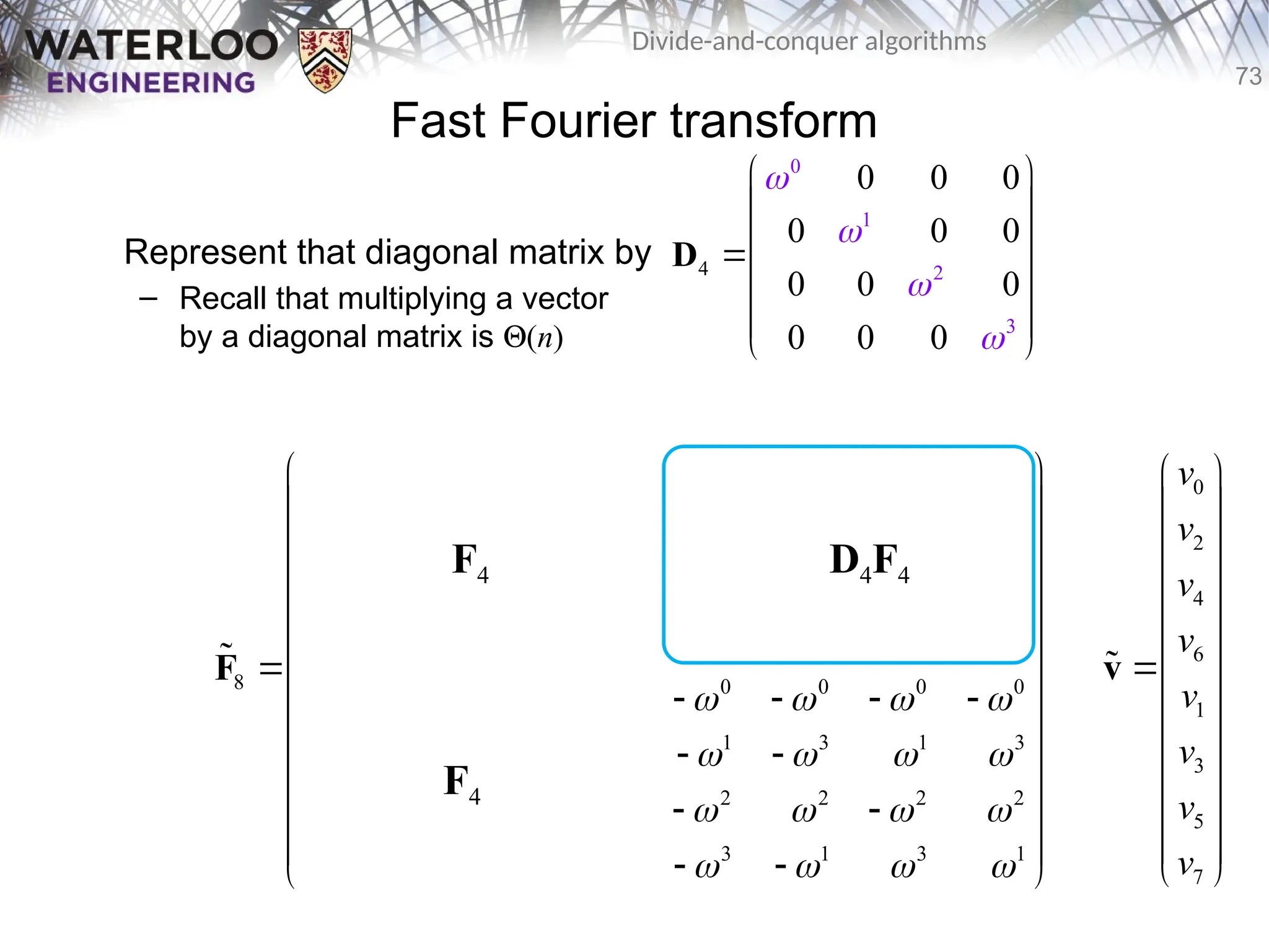
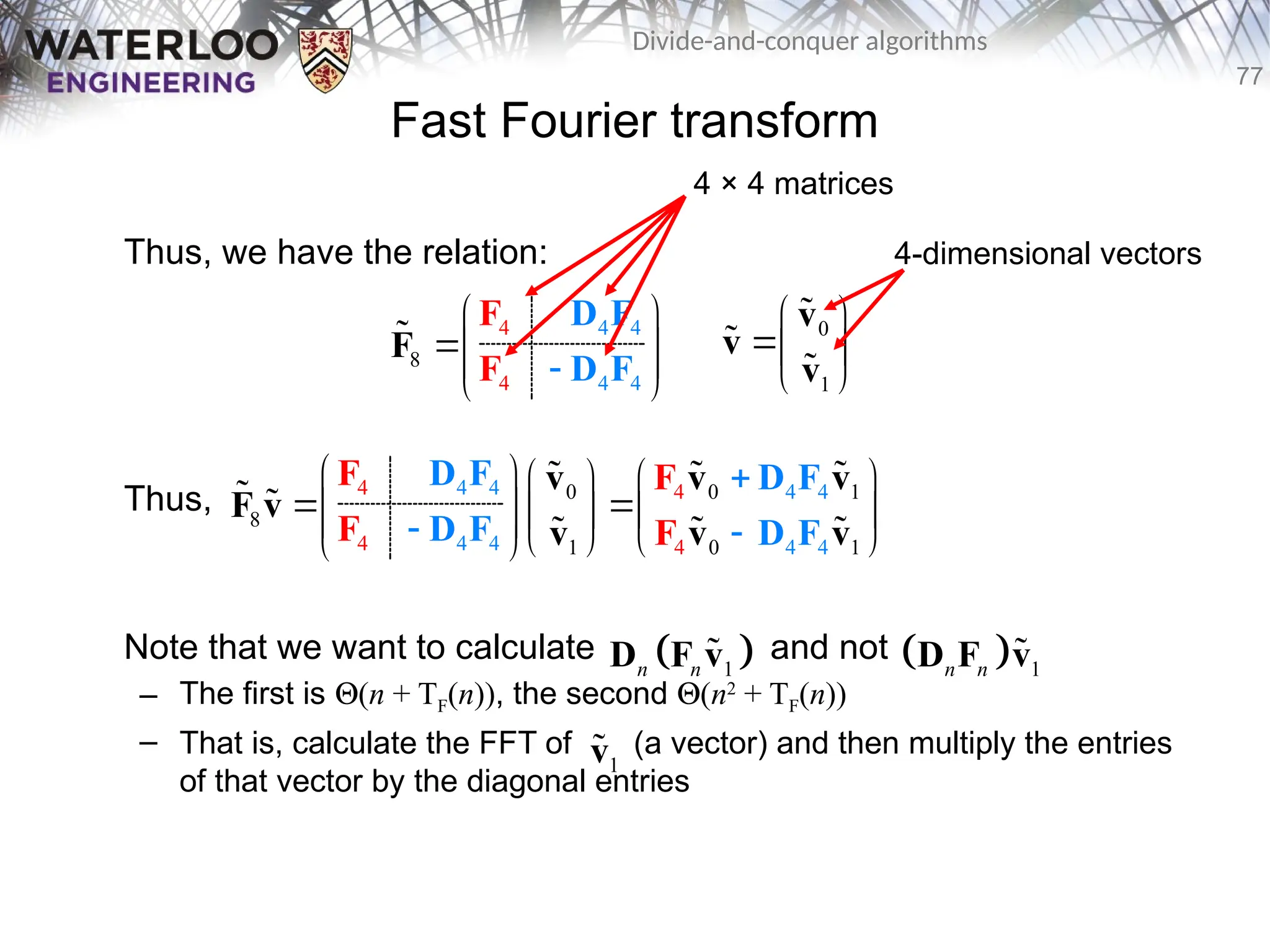
Thus, we have the relation:
Thus,
Note that we want to calculate and not
– The first is Q(n + TF(n)), the second Q(n2
+ TF(n))
– That is, calculate the FFT of (a vector) and then multiply the entries
of that vector by the diagonal entries
4
4
8
4
4
4
4
F
D F
D F
F
F
0
1
v
v
v
0 1
4 4
4
4 4 4 4
4
0
8
0
4 4 4 1
1
4
D F D F
F
D F D F
v v
v
F v
v v
v
F
F F
1
n n
D F v
1
n n
D F v
4 × 4 matrices
4-dimensional vectors
1
v
78.
78
Divide-and-conquer algorithms
Fast Fouriertransform
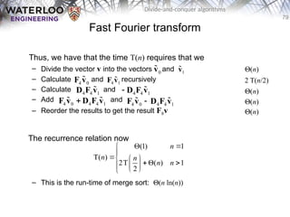
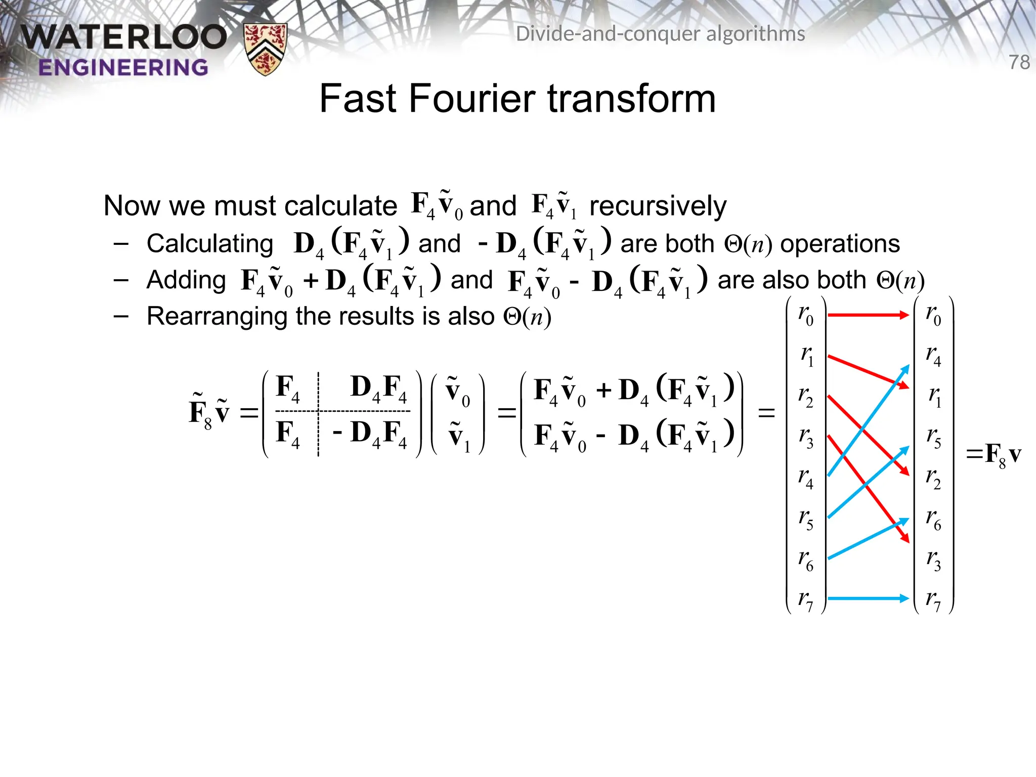
Now we must calculate and recursively
– Calculating and are both Q(n) operations
– Adding and are also both Q(n)
– Rearranging the results is also Q(n)
4 0
F v
4 1
F v
4 4 1
D F v
4 4 1
D F v
4 0 4 4 1
F v D F v
4 0 4 4 1
F v D F v
4 4 4 4 0 4 4 1
0
8
4 4 4 4 0 4 4 1
1
F D F F v D F v
v
F v
F D F F v D F v
v
0 0
1 4
2 1
3 5
8
4 2
5 6
6 3
7 7
r r
r r
r r
r r
r r
r r
r r
r r
F v
79.
79
Divide-and-conquer algorithms
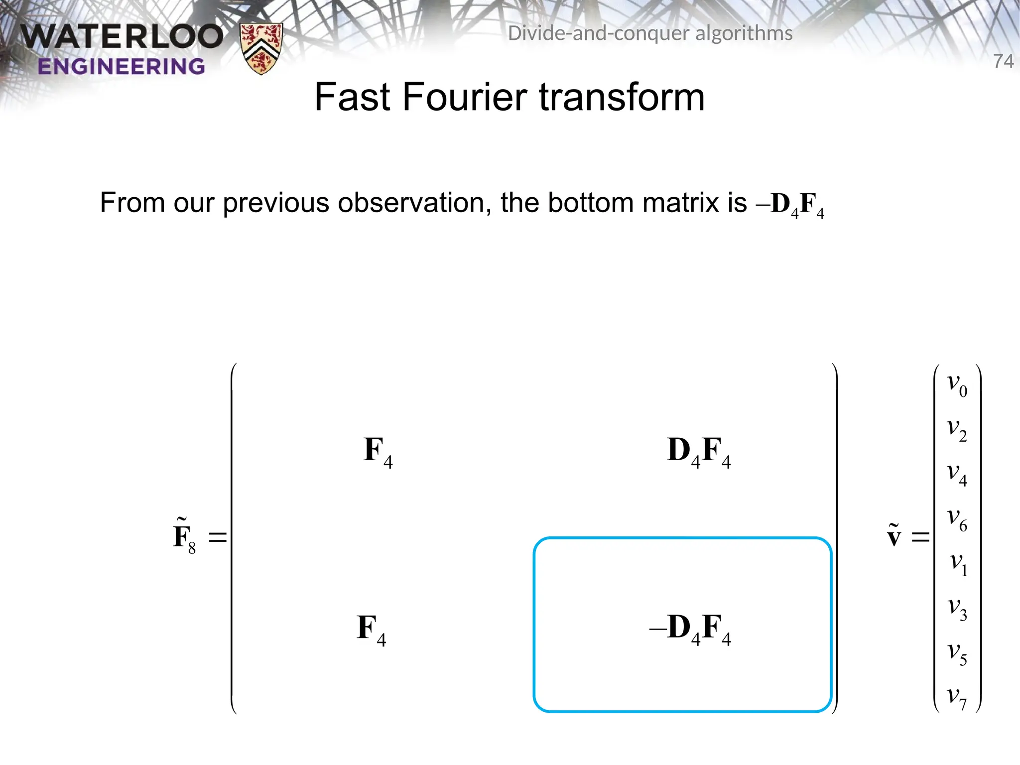
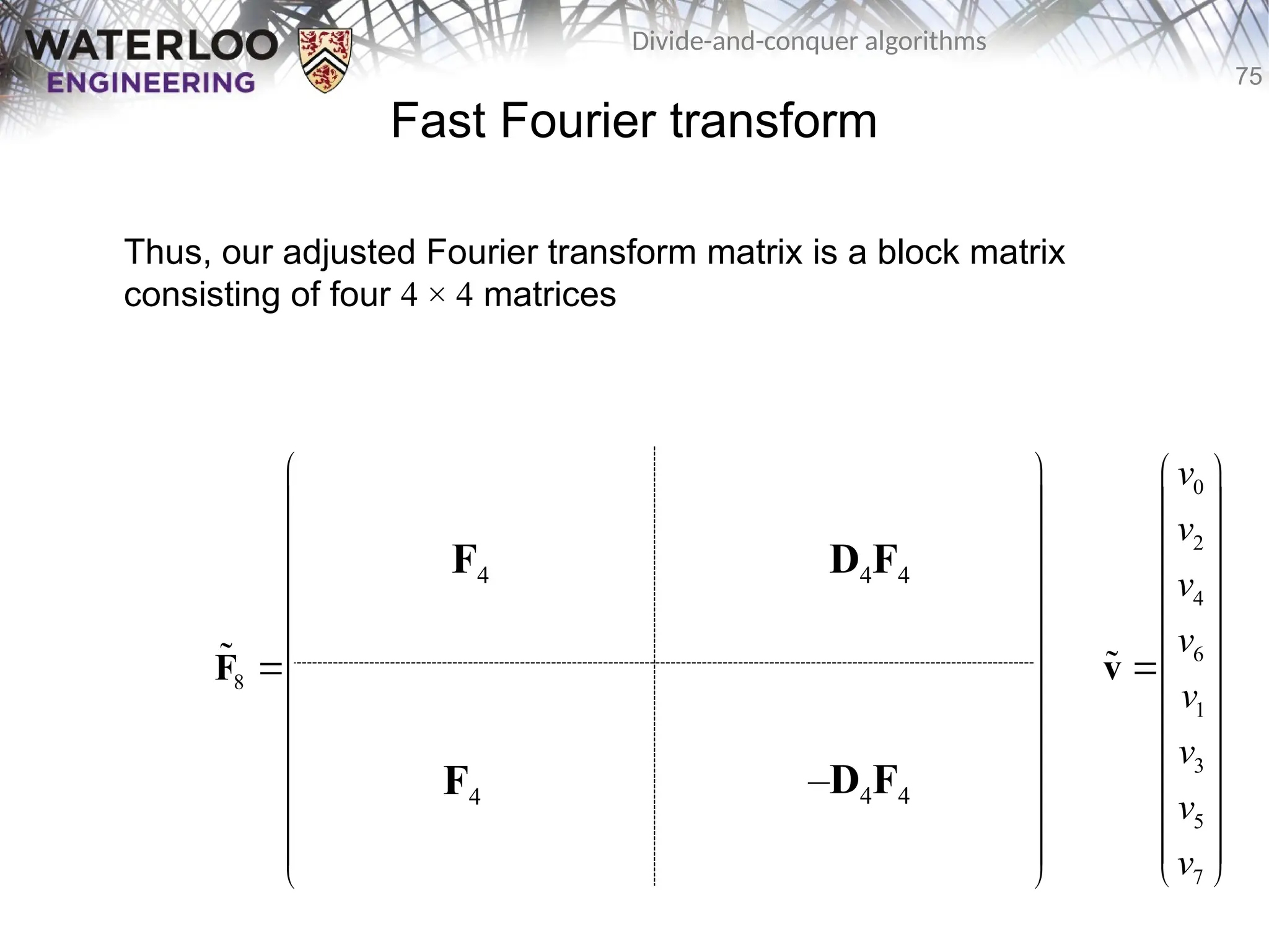
Fast Fouriertransform
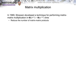
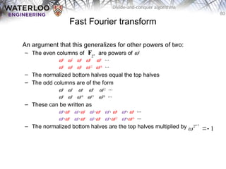
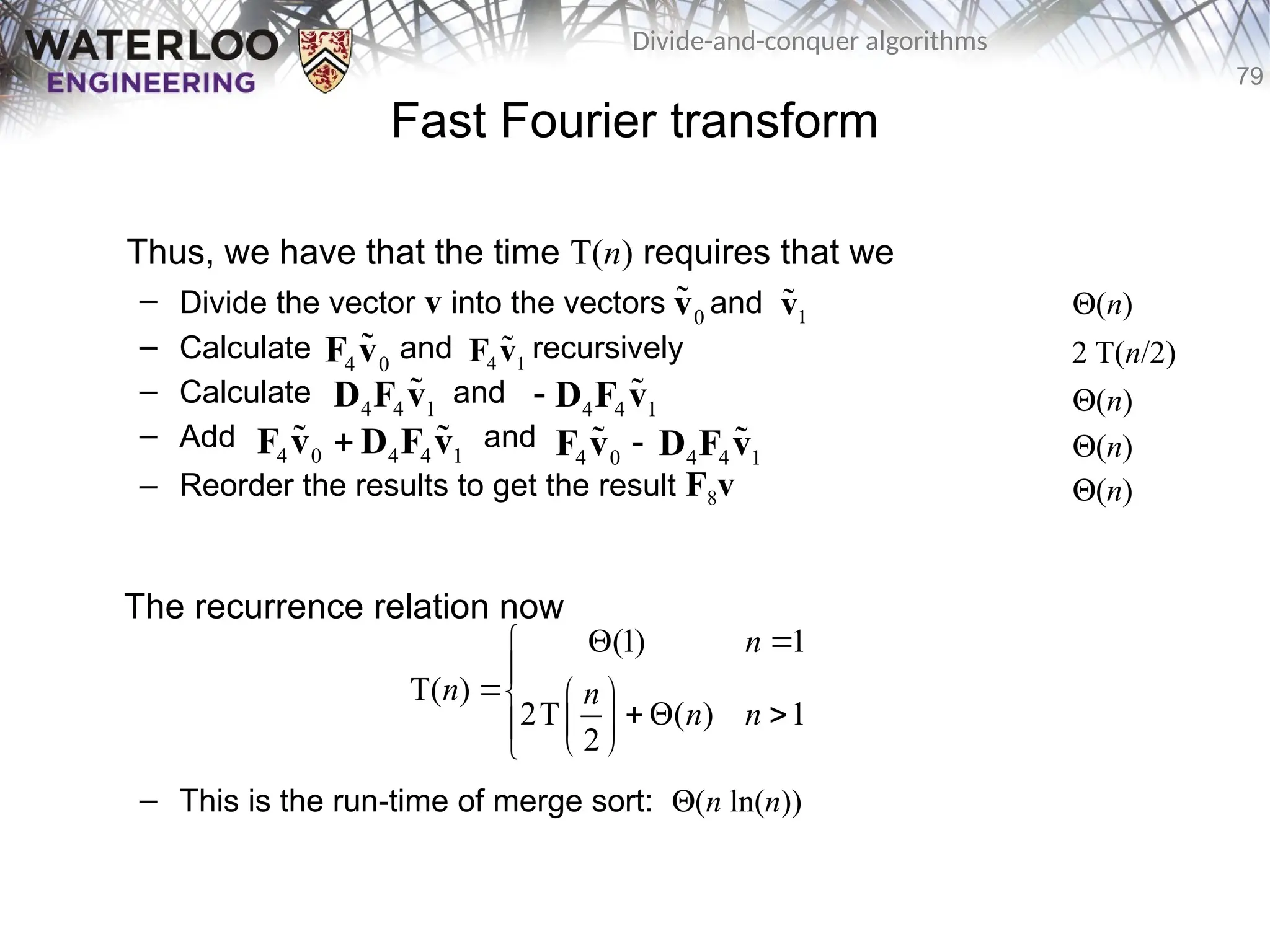
Thus, we have that the time T(n) requires that we
– Divide the vector v into the vectors and
– Calculate and recursively
– Calculate and
– Add and
– Reorder the results to get the result F8v
The recurrence relation now
– This is the run-time of merge sort: Q(n ln(n))
4 0
F v
4 1
F v
4 4 1
D F v
4 4 1
D F v
4 0 4 4 1
F v D F v
4 0 4 4 1
F v D F v
0
v
1
v
Q(n)
2 T(n/2)
Q(n)
Q(n)
Q(n)
(1) 1
T( )
2T ( ) 1
2
n
n n
n n
80.
80
Divide-and-conquer algorithms
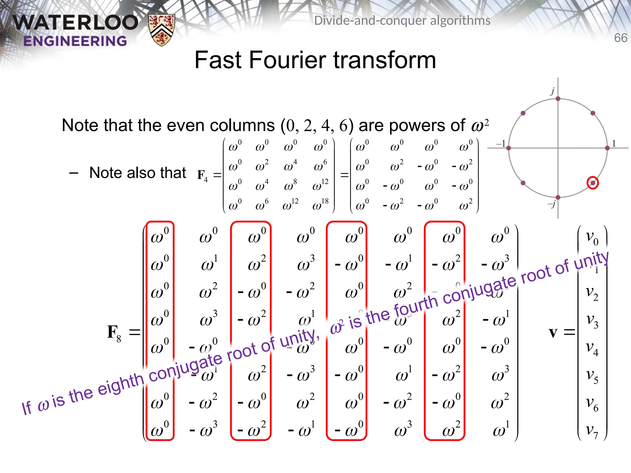
Fast Fouriertransform
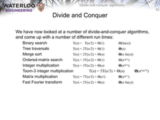
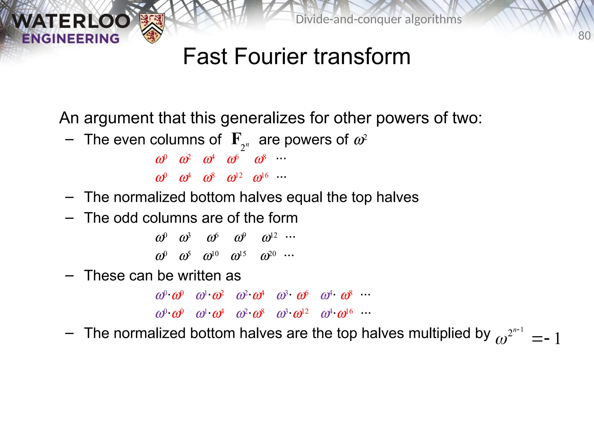
An argument that this generalizes for other powers of two:
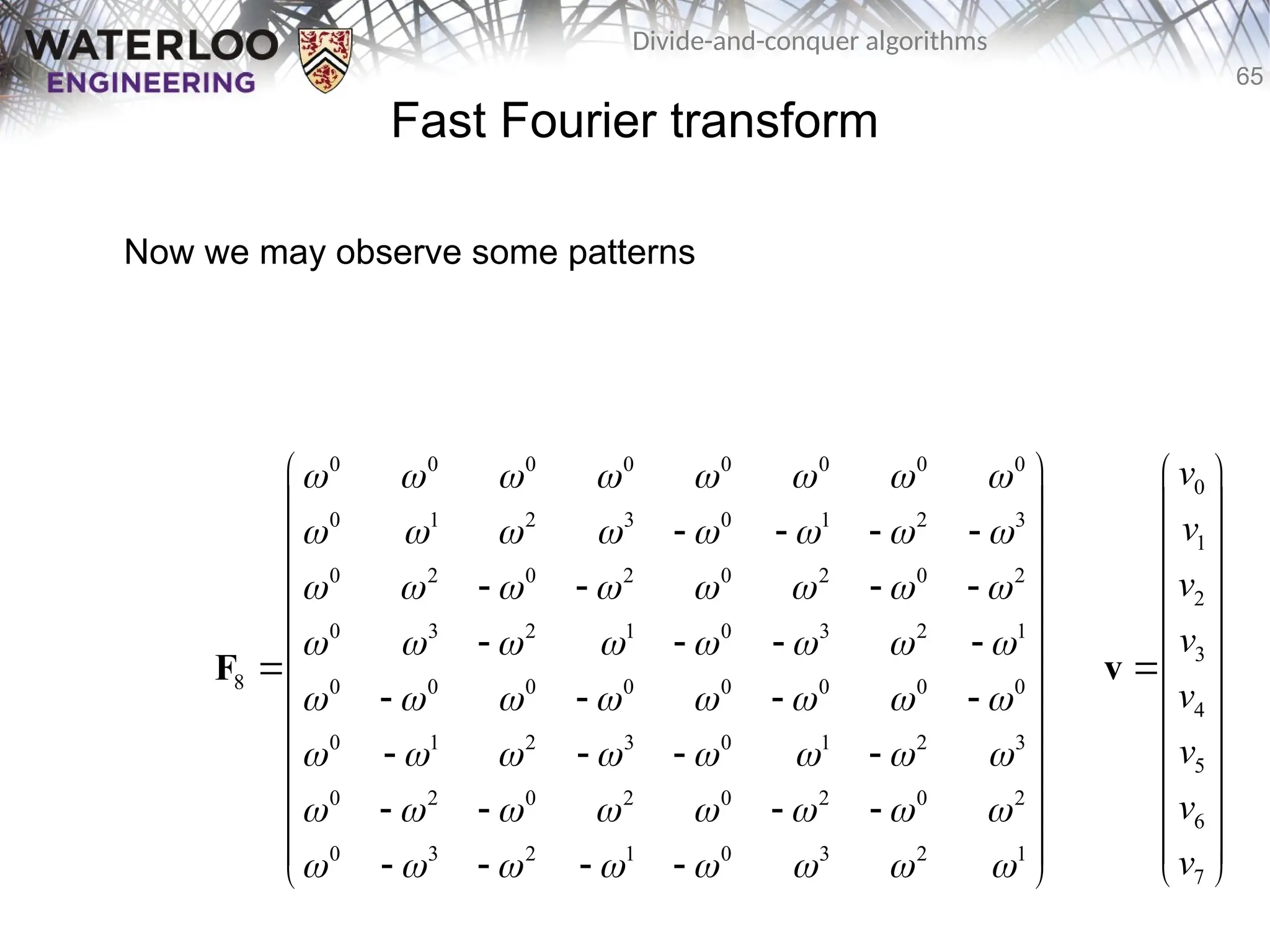
– The even columns of are powers of w2
w0
w2
w4
w6
w8
···
w0
w4
w8
w12
w16
···
– The normalized bottom halves equal the top halves
– The odd columns are of the form
w0
w3
w6
w9
w12
···
w0
w5
w10
w15
w20
···
– These can be written as
w0
·w0
w1
·w2
w2
·w4
w3
· w6
w4
· w8
···
w0
·w0
w1
·w4
w2
·w8
w3
·w12
w4
·w16
···
– The normalized bottom halves are the top halves multiplied by
2n
F
1
2
1
n
81.
81
Divide-and-conquer algorithms
Fast Fouriertransform
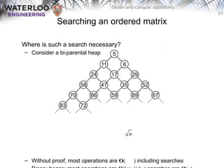
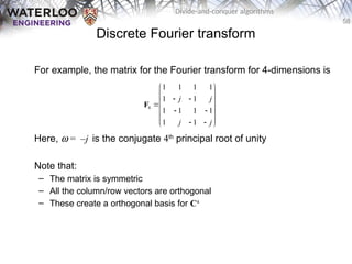
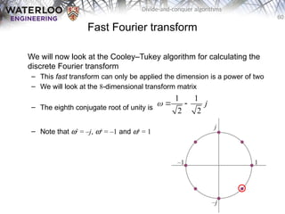
void FFT( std::complex<double> *array, int n ) {
if ( n == 1 ) return;
std::complex<double> even[n/2];
std::complex<double> odd[n/2];
for ( int k = 0; k < n/2; ++k ) {
even[k] = array[2*k];
odd[k] = array[2*k + 1];
}
FFT( even, n/2 );
FFT( odd, n/2 );
double const PI = 4.0*std::atan( 1.0 );
std::complex<double> w = 1.0;
std::complex<double> wn = std::exp( std::complex<double>( 0.0, -2.0*PI/n ) );
for ( int k = 0; k < n/2; ++k ) {
array[k] = even[k] + w*odd[k];
array[n/2 + k] = even[k] - w*odd[k];
w = w * wn;
}
}
( )
n
( )
n
(1)
2
T
2 n
(1)
(1)
82.
82
Divide-and-conquer algorithms
Divide andConquer
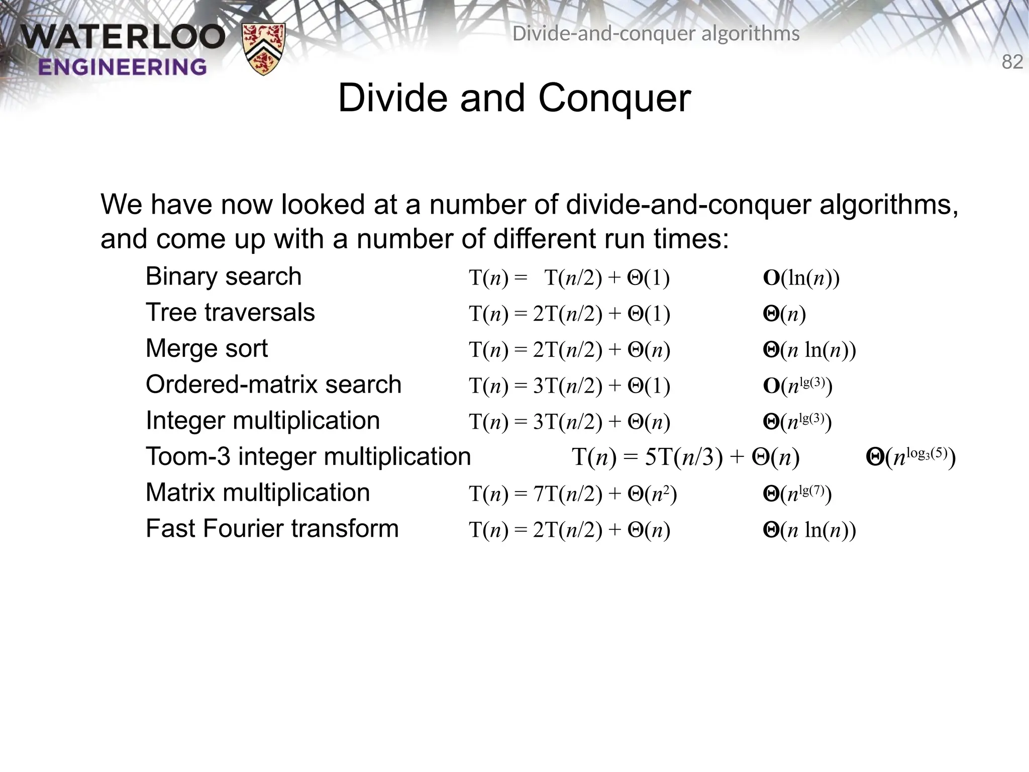
We have now looked at a number of divide-and-conquer algorithms,
and come up with a number of different run times:
Binary search T(n) = T(n/2) + Q(1) O(ln(n))
Tree traversals T(n) = 2T(n/2) + Q(1) Q(n)
Merge sort T(n) = 2T(n/2) + Q(n) Q(n ln(n))
Ordered-matrix search T(n) = 3T(n/2) + Q(1) O(nlg(3)
)
Integer multiplication T(n) = 3T(n/2) + Q(n) Q(nlg(3)
)
Toom-3 integer multiplication T(n) = 5T(n/3) + Q(n) Q(nlog3(5)
)
Matrix multiplication T(n) = 7T(n/2) + Q(n2
) Q(nlg(7)
)
Fast Fourier transform T(n) = 2T(n/2) + Q(n) Q(n ln(n))
83.
83
Divide-and-conquer algorithms
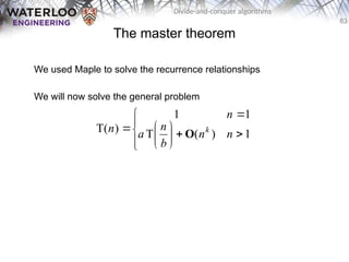
The mastertheorem
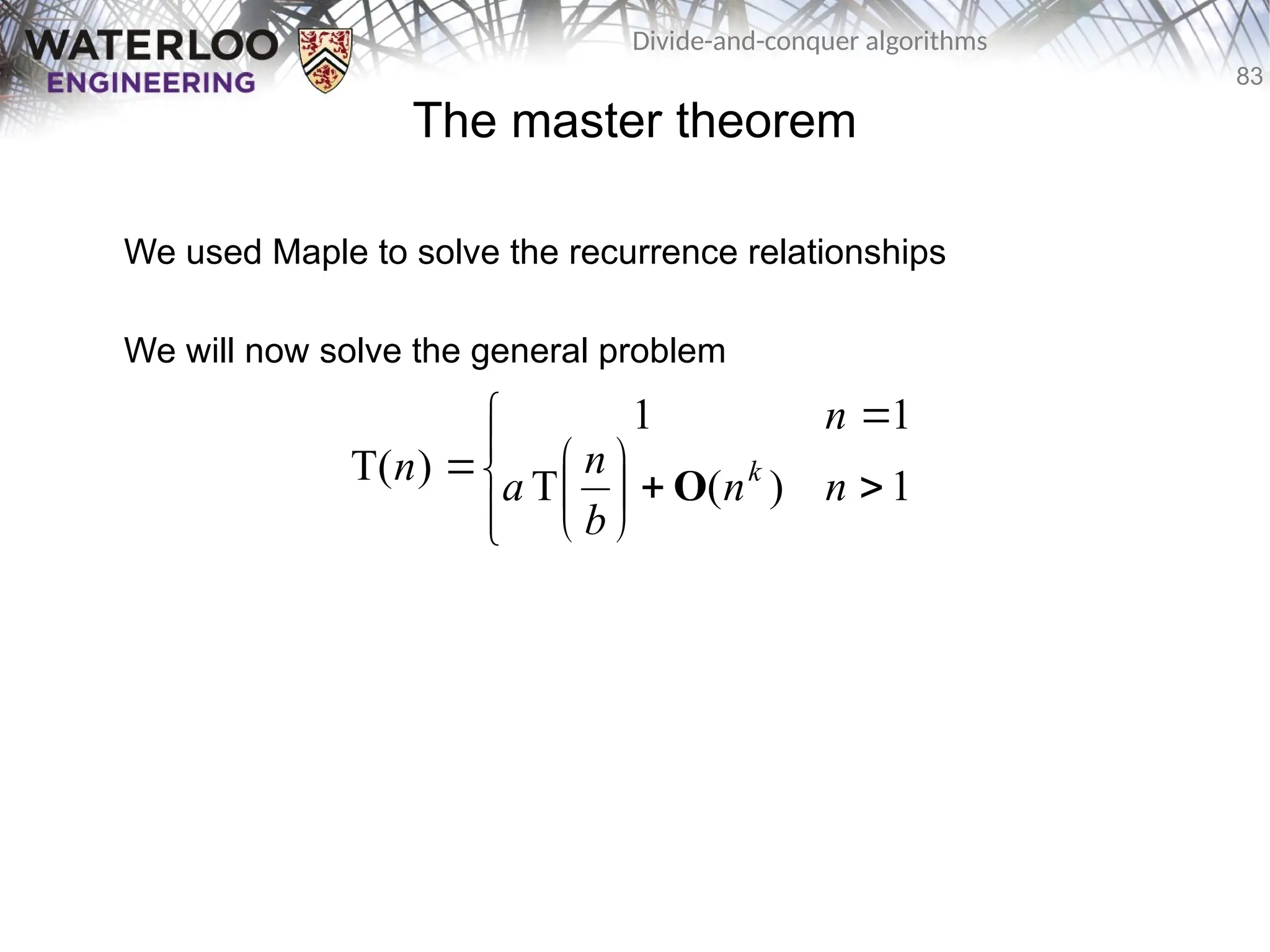
We used Maple to solve the recurrence relationships
We will now solve the general problem
1
)
(
T
1
1
)
T( n
n
b
n
a
n
n k
O
84.
84
Divide-and-conquer algorithms
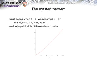
The mastertheorem
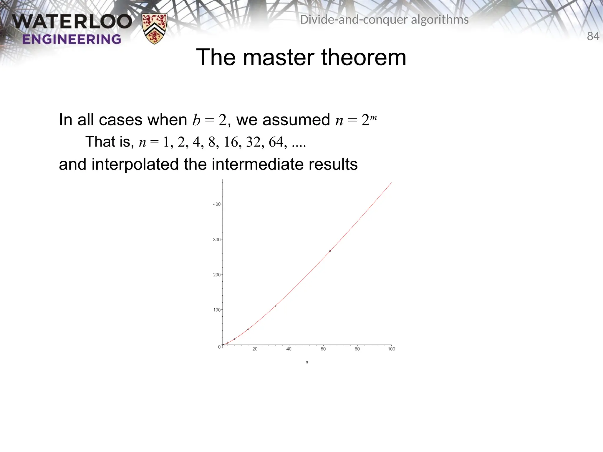
In all cases when b = 2, we assumed n = 2m
That is, n = 1, 2, 4, 8, 16, 32, 64, ....
and interpolated the intermediate results
85.
85
Divide-and-conquer algorithms
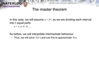
The mastertheorem
In this case, we will assume n = bm
, as we are dividing each interval
into b equal parts
n = 1, b, b2
, b3
, ...
As before, we will interpolate intermediate behaviour
– Thus, we will solve T(bm
) and use this to approximate T(n)
86.
86
Divide-and-conquer algorithms
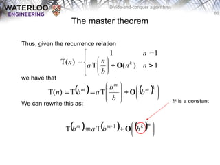
The mastertheorem
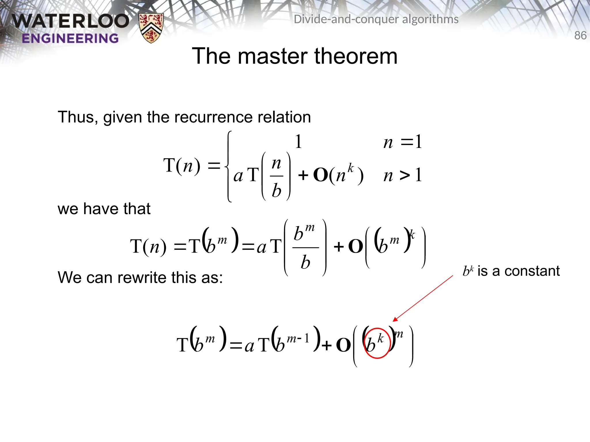
Thus, given the recurrence relation
we have that
We can rewrite this as:
1
)
(
T
1
1
)
T( n
n
b
n
a
n
n k
O
k
m
m
m
b
b
b
a
b
n O
T
T
)
T(
m
k
m
m
b
b
a
b O
1
T
T
bk
is a constant
87.
87
Divide-and-conquer algorithms
The mastertheorem
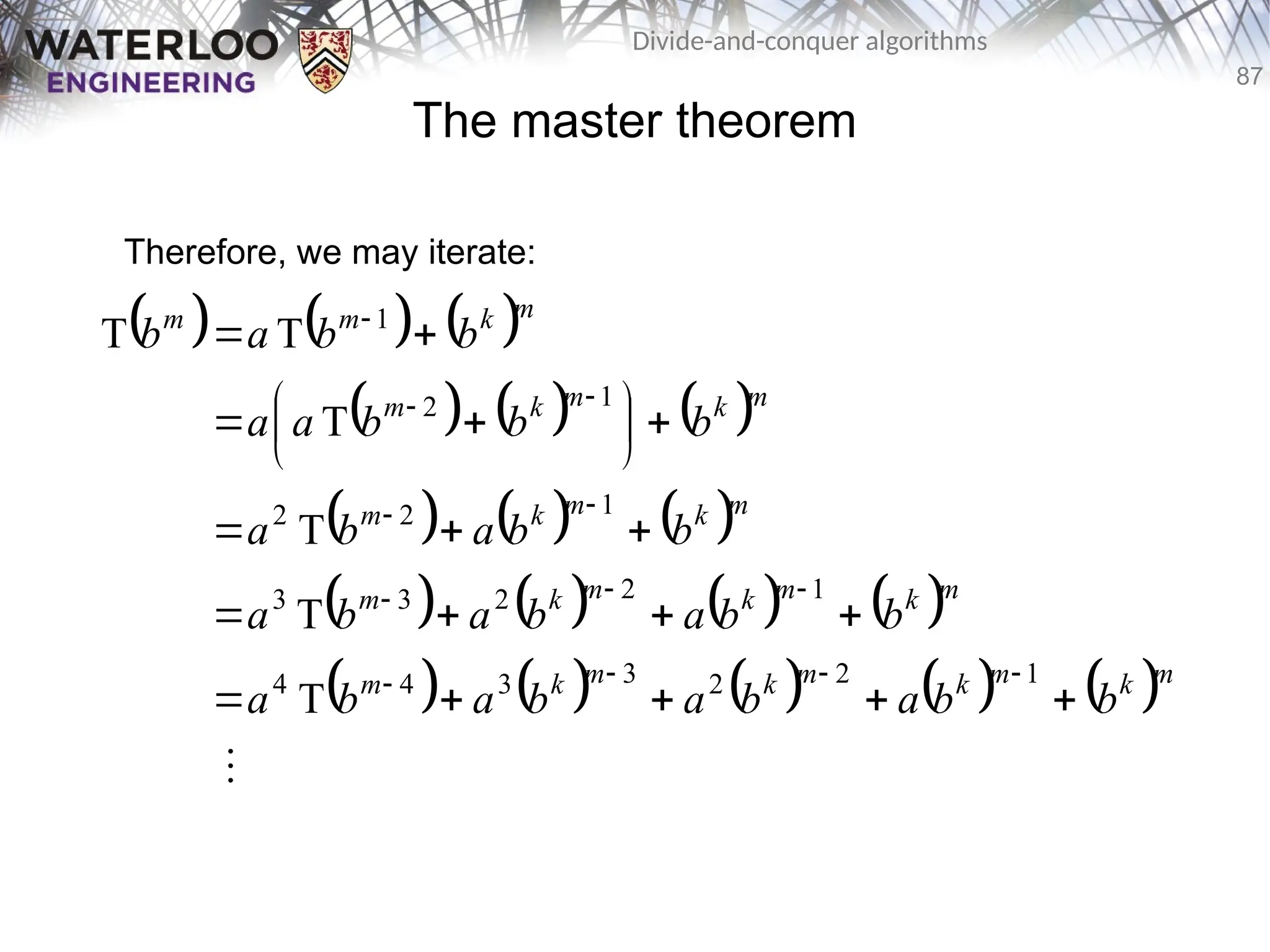
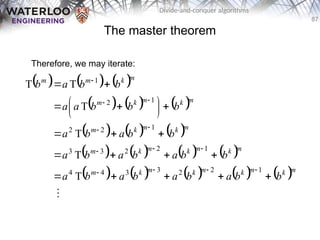
Therefore, we may iterate:
m
k
m
k
m
k
m
k
m
m
k
m
k
m
k
m
m
k
m
k
m
m
k
m
k
m
m
k
m
m
b
b
a
b
a
b
a
b
a
b
b
a
b
a
b
a
b
b
a
b
a
b
b
b
a
a
b
b
a
b
1
2
2
3
3
4
4
1
2
2
3
3
1
2
2
1
2
1
T
T
T
T
T
T
88.
88
Divide-and-conquer algorithms
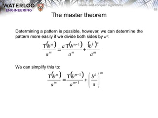
The mastertheorem
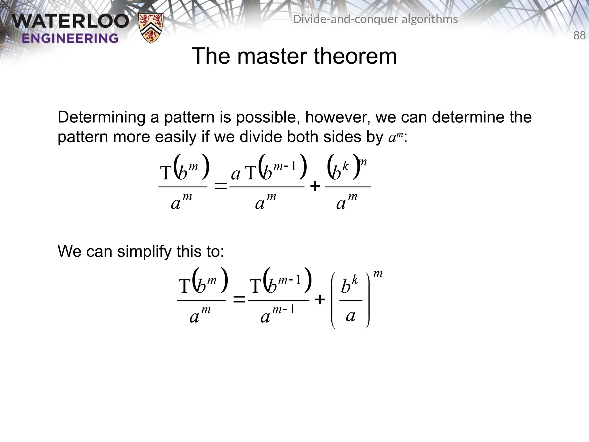
Determining a pattern is possible, however, we can determine the
pattern more easily if we divide both sides by am
:
We can simplify this to:
m
m
k
m
m
m
m
a
b
a
b
a
a
b
1
T
T
m
k
m
m
m
m
a
b
a
b
a
b
1
1
T
T
89.
89
Divide-and-conquer algorithms
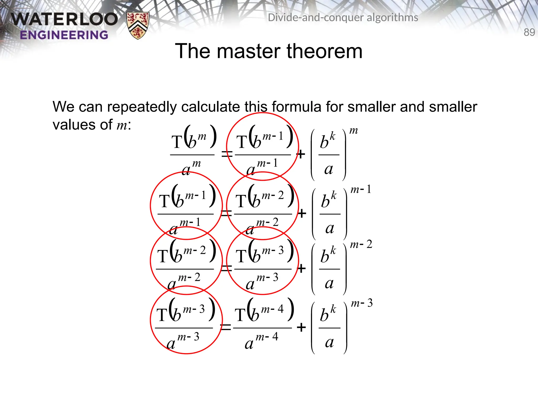
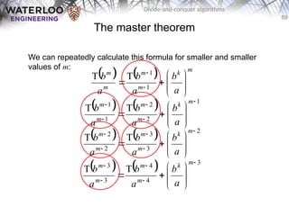
The mastertheorem
We can repeatedly calculate this formula for smaller and smaller
values of m:
m
k
m
m
m
m
a
b
a
b
a
b
1
1
T
T
1
2
2
1
1
T
T
m
k
m
m
m
m
a
b
a
b
a
b
2
3
3
2
2
T
T
m
k
m
m
m
m
a
b
a
b
a
b
3
4
4
3
3
T
T
m
k
m
m
m
m
a
b
a
b
a
b
90.
90
Divide-and-conquer algorithms
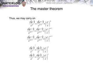
The mastertheorem
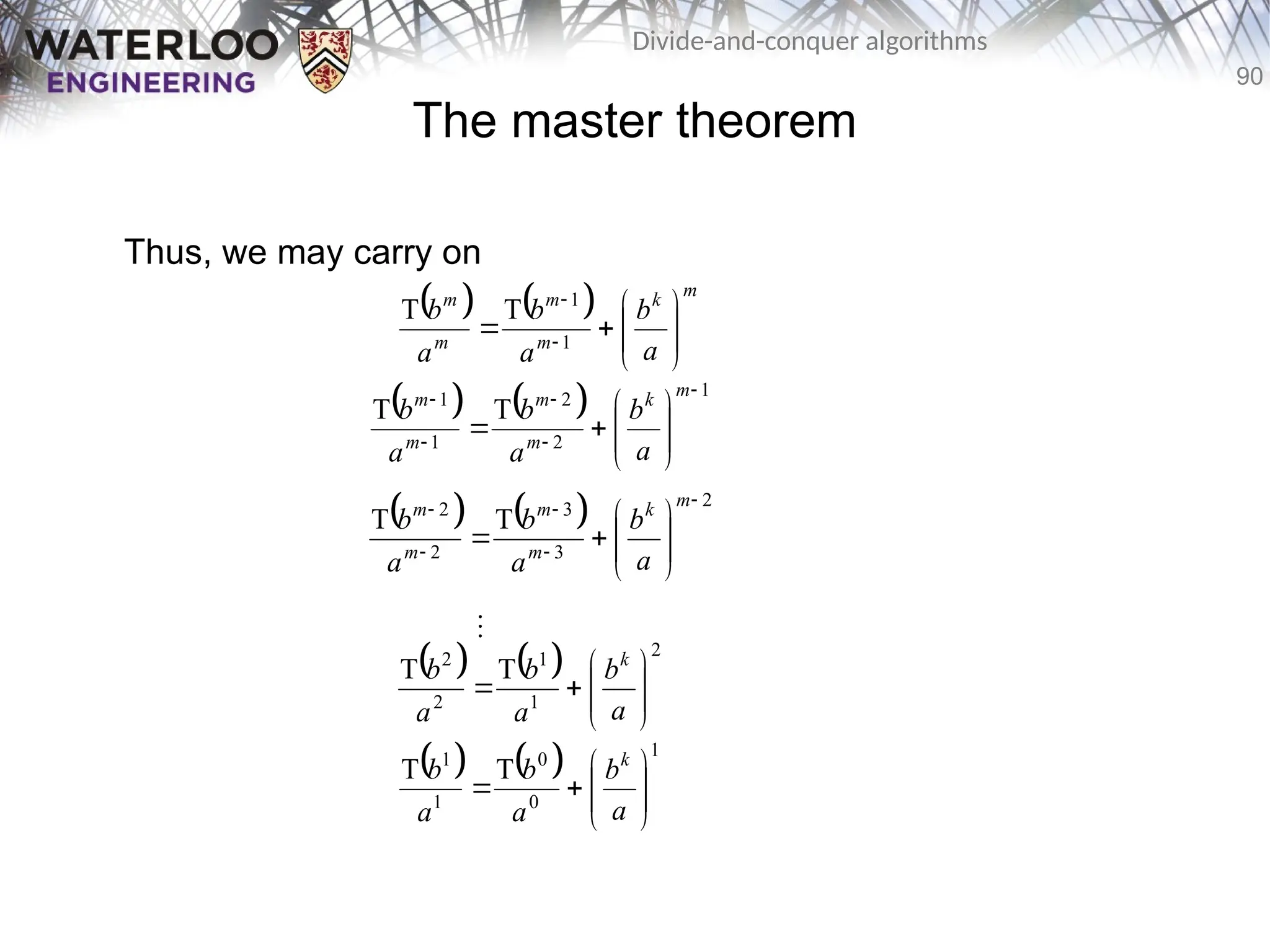
Thus, we may carry on
m
k
m
m
m
m
a
b
a
b
a
b
1
1
T
T
1
2
2
1
1
T
T
m
k
m
m
m
m
a
b
a
b
a
b
2
3
3
2
2
T
T
m
k
m
m
m
m
a
b
a
b
a
b
1
0
0
1
1
T
T
a
b
a
b
a
b k
2
1
1
2
2
T
T
a
b
a
b
a
b k
91.
91
Divide-and-conquer algorithms
The mastertheorem
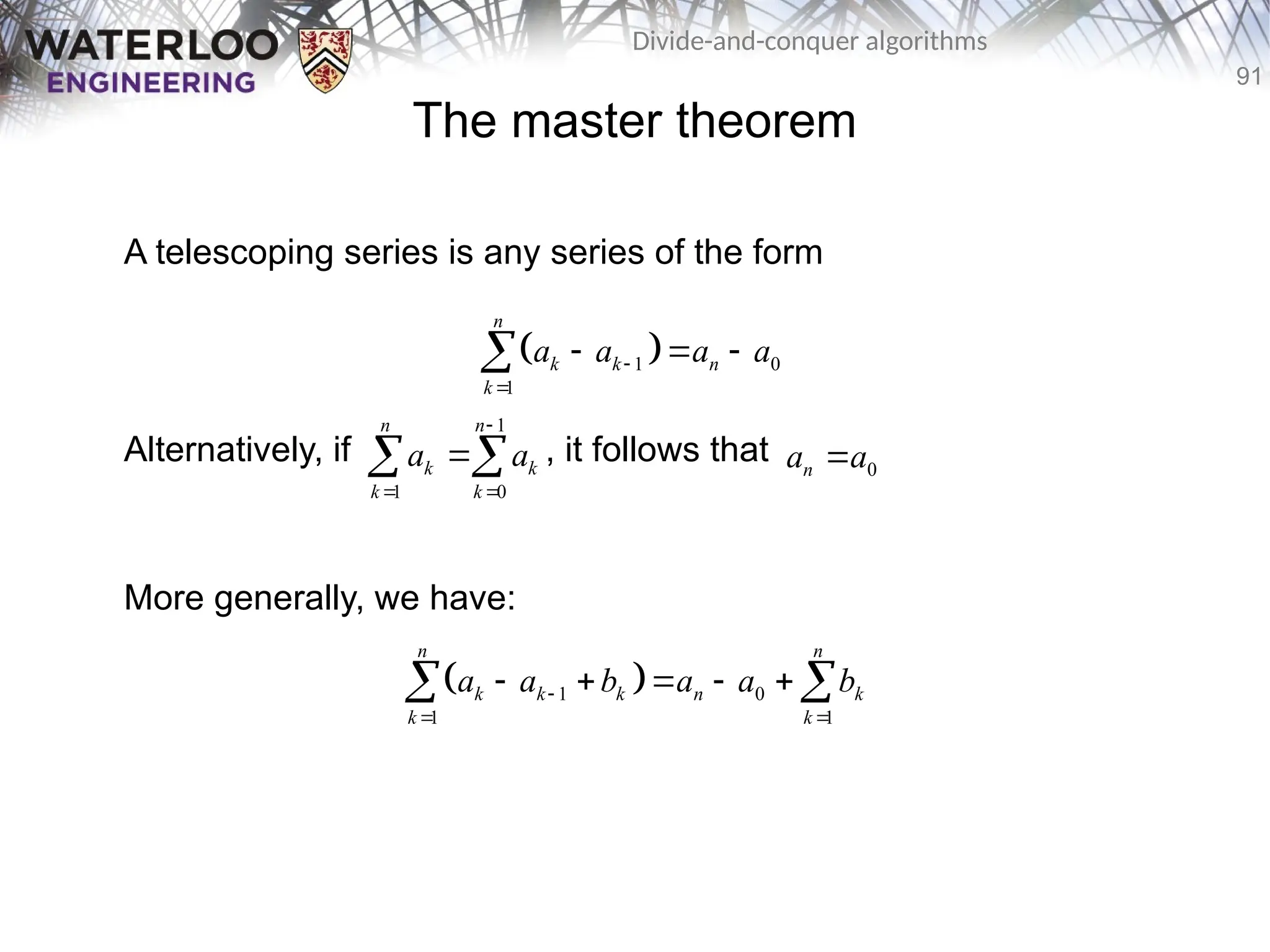
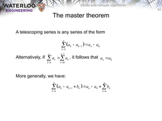
A telescoping series is any series of the form
Alternatively, if , it follows that
More generally, we have:
1 0
1
n
k k n
k
a a a a
1 0
1 1
n n
k k k n k
k k
a a b a a b
1
1 0
n n
k k
k k
a a
0
n
a a
92.
92
Divide-and-conquer algorithms
The mastertheorem
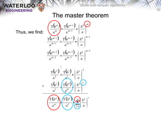
Thus, we find:
+
m
k
m
m
m
m
a
b
a
b
a
b
1
1
T
T
1
2
2
1
1
T
T
m
k
m
m
m
m
a
b
a
b
a
b
2
3
3
2
2
T
T
m
k
m
m
m
m
a
b
a
b
a
b
1
0
0
1
1
T
T
a
b
a
b
a
b k
2
1
1
2
2
T
T
a
b
a
b
a
b k
0
0
1
T T
m k
m
m
b b b
a a a
93.
93
Divide-and-conquer algorithms
The mastertheorem
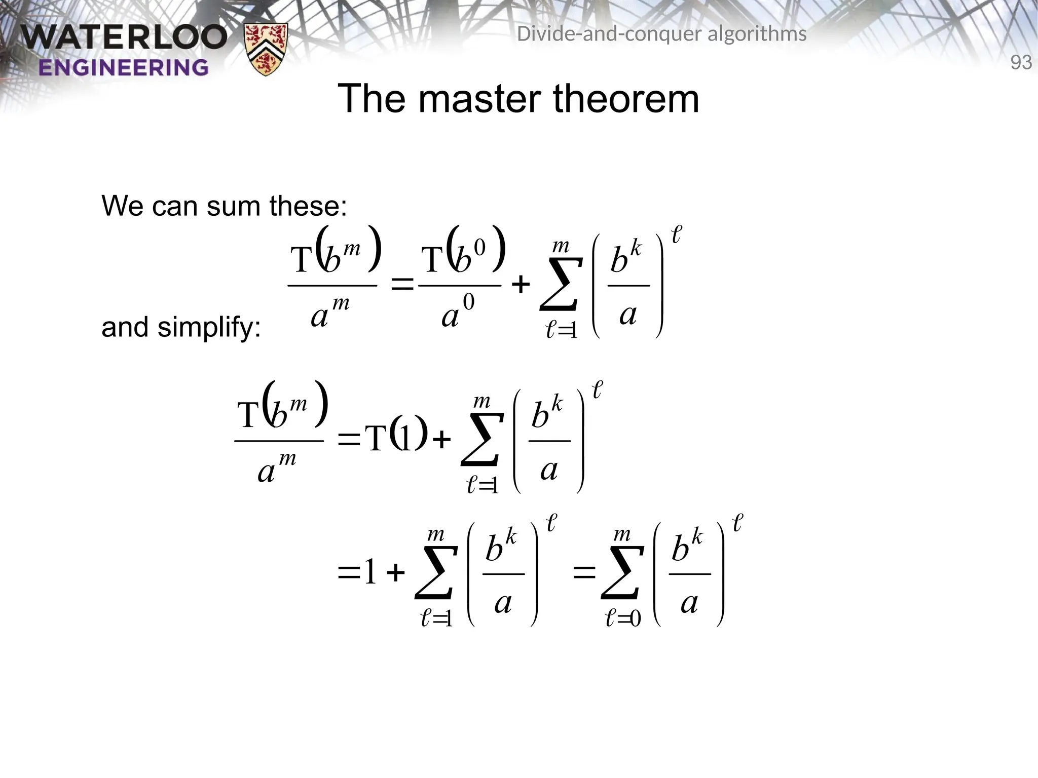
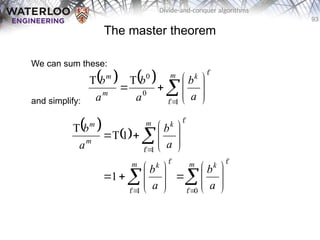
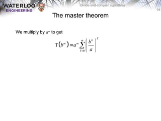
We can sum these:
and simplify:
m k
m
m
a
b
a
b
a
b
1
0
0
T
T
m k
m k
m k
m
m
a
b
a
b
a
b
a
b
0
1
1
1
1
T
T
95
Divide-and-conquer algorithms
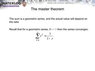
The mastertheorem
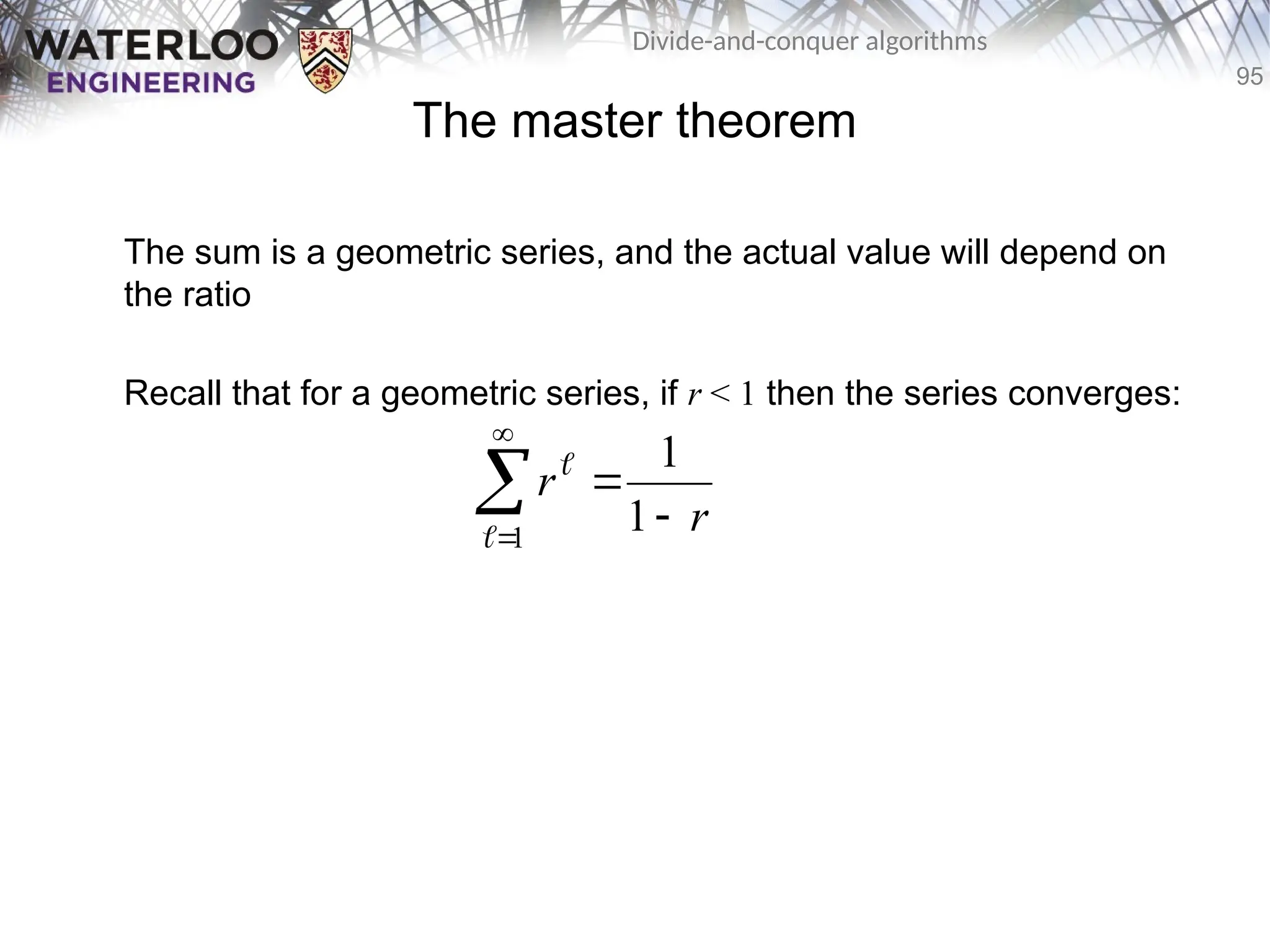
The sum is a geometric series, and the actual value will depend on
the ratio
Recall that for a geometric series, if r < 1 then the series converges:
r
r
1
1
1
96.
96
Divide-and-conquer algorithms
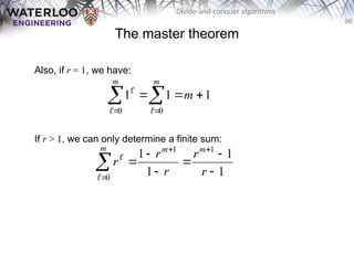
The mastertheorem
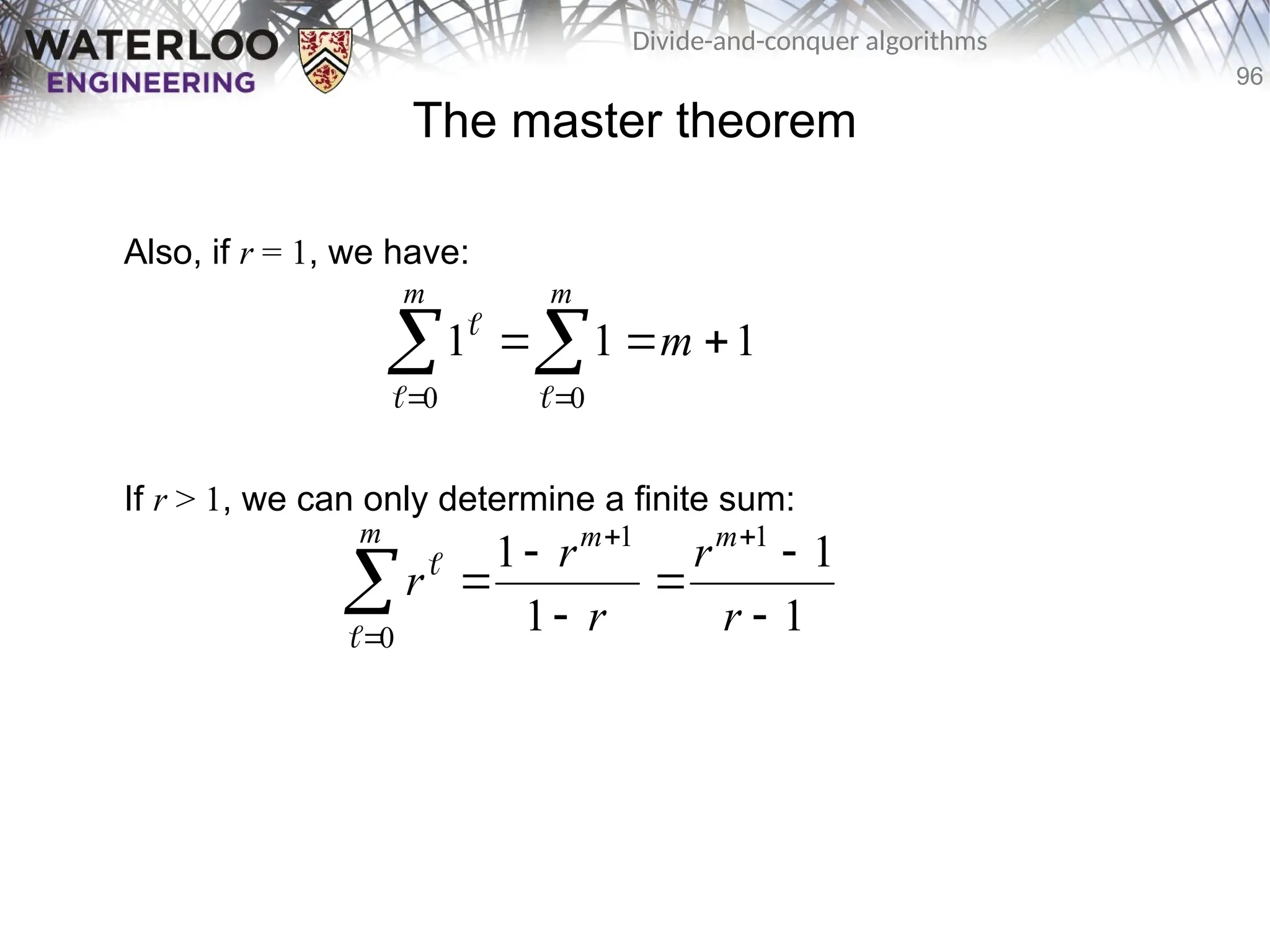
Also, if r = 1, we have:
If r > 1, we can only determine a finite sum:
1
1
1
0
0
m
m
m
1
1
1
1 1
1
0
r
r
r
r
r
m
m
m
98
Divide-and-conquer algorithms
The mastertheorem
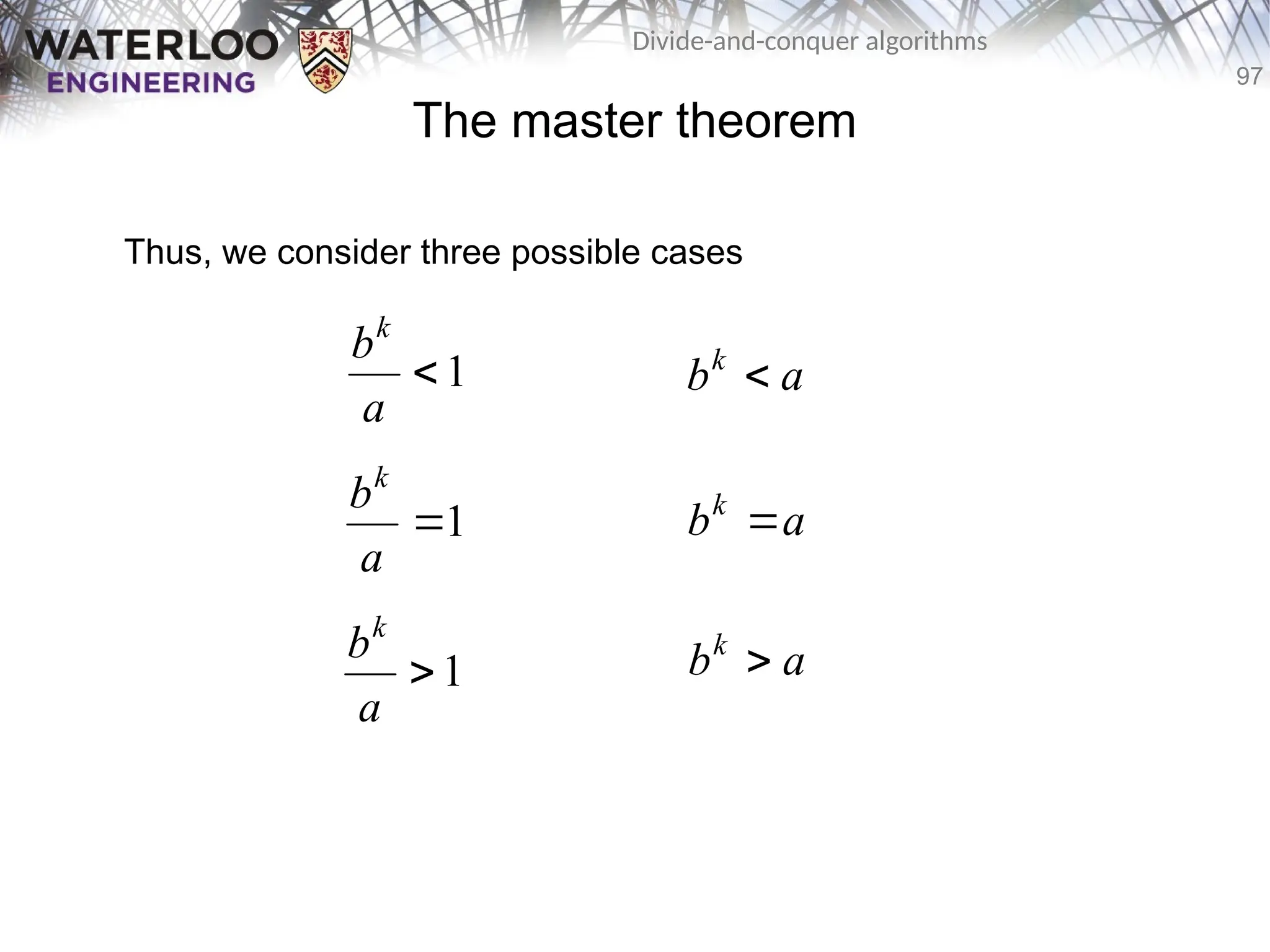
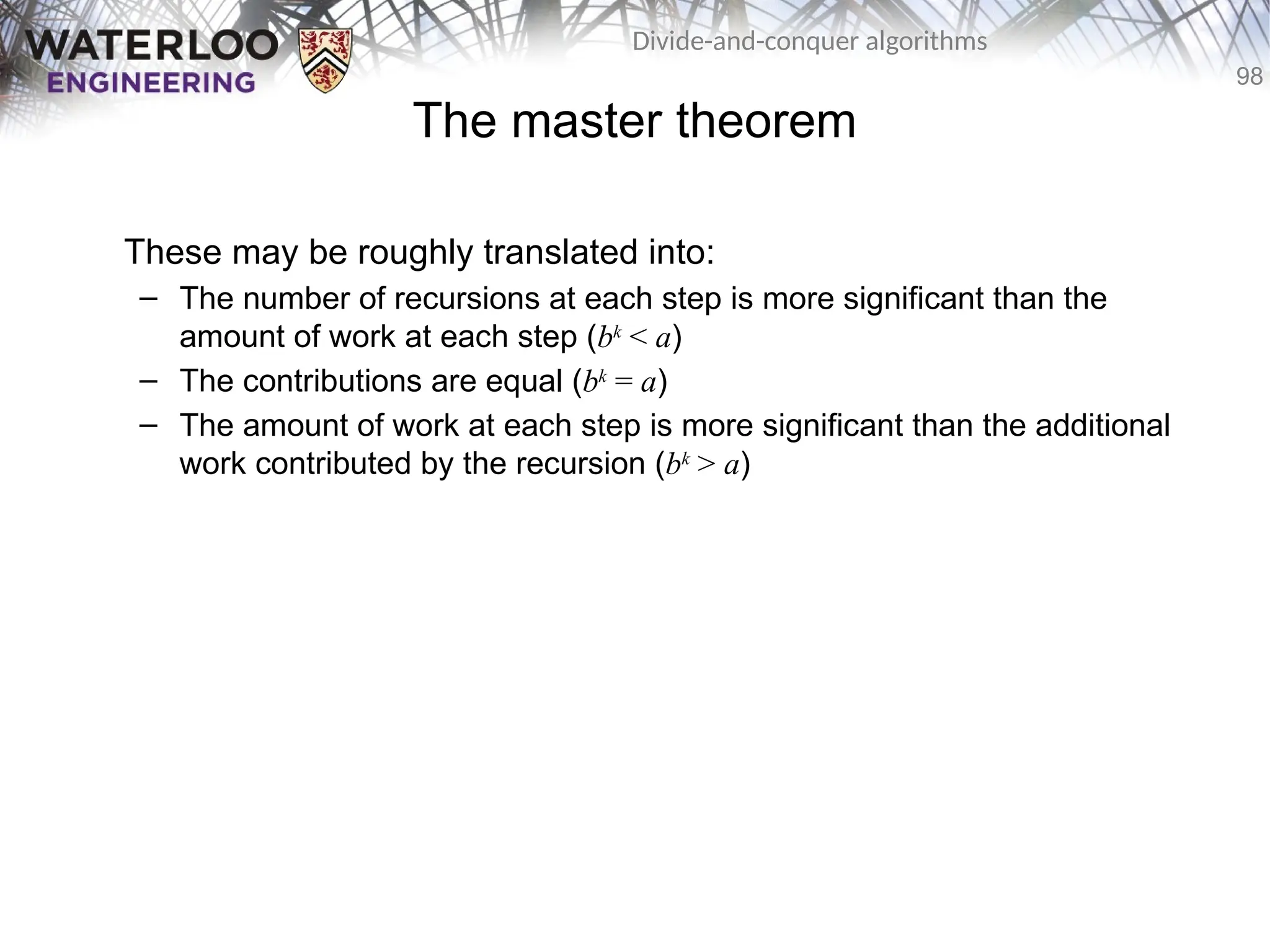
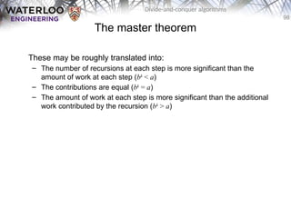
These may be roughly translated into:
– The number of recursions at each step is more significant than the
amount of work at each step (bk
< a)
– The contributions are equal (bk
= a)
– The amount of work at each step is more significant than the additional
work contributed by the recursion (bk
> a)
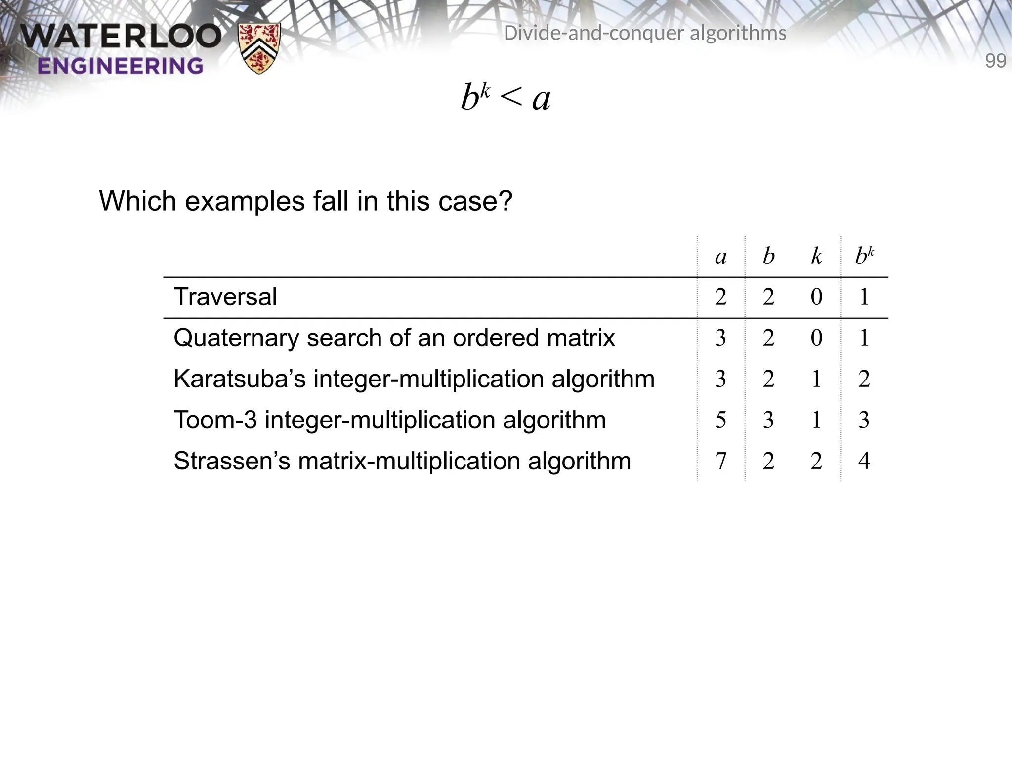
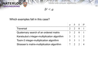
99.
99
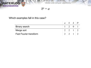
Divide-and-conquer algorithms
bk
< a
Whichexamples fall in this case?
a b k bk
Traversal 2 2 0 1
Quaternary search of an ordered matrix 3 2 0 1
Karatsuba’s integer-multiplication algorithm 3 2 1 2
Toom-3 integer-multiplication algorithm 5 3 1 3
Strassen’s matrix-multiplication algorithm 7 2 2 4
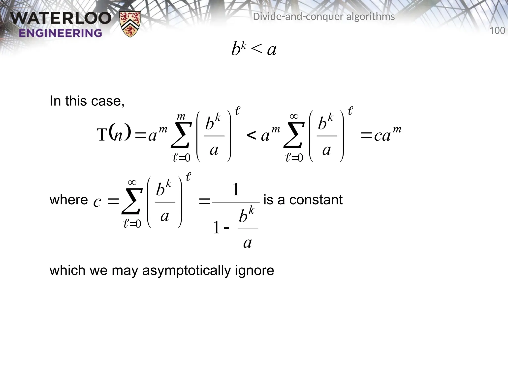
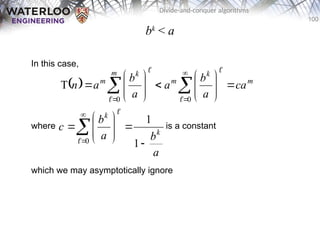
100.
100
Divide-and-conquer algorithms
bk
< a
Inthis case,
where is a constant
which we may asymptotically ignore
m
k
m
m k
m
ca
a
b
a
a
b
a
n
0
0
T
0 1
1
a
b
a
b
c k
k
104
Divide-and-conquer algorithms
bk
= a
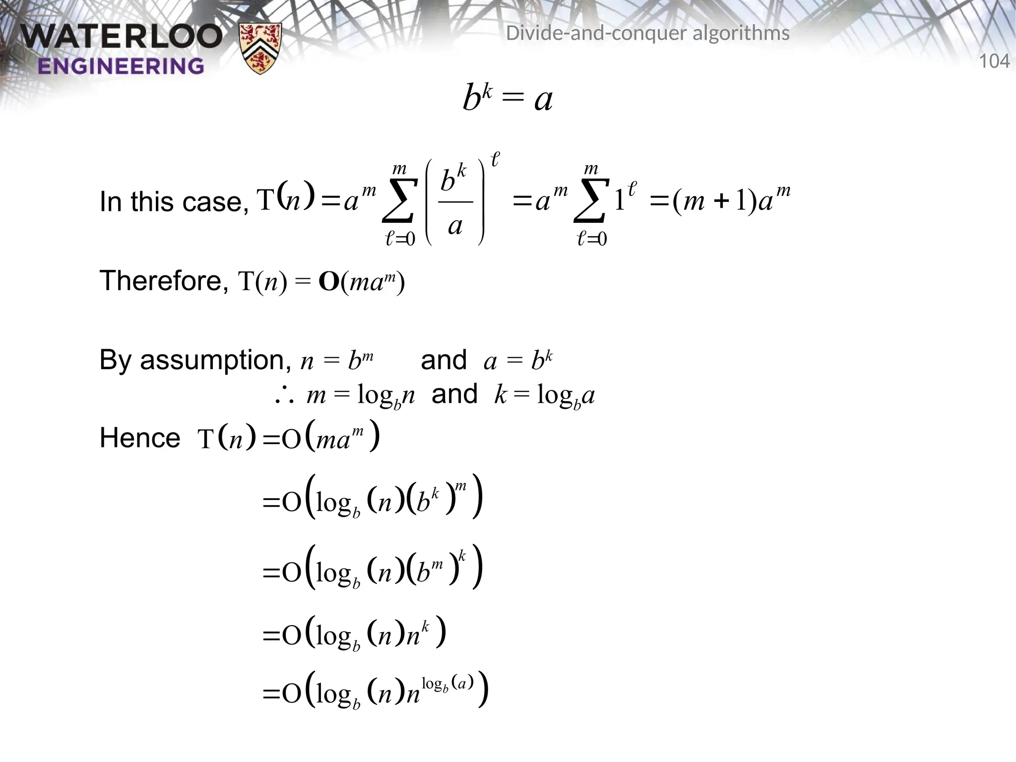
Inthis case,
Therefore, T(n) = O(mam
)
By assumption, n = bm
and a = bk
∴ m = logbn and k = logba
Hence
m
m
m
m k
m
a
m
a
a
b
a
n )
1
(
1
T
0
0
log
T O
O log
O log
O log
O log b
m
m
k
b
k
m
b
k
b
a
b
n ma
n b
n b
n n
n n
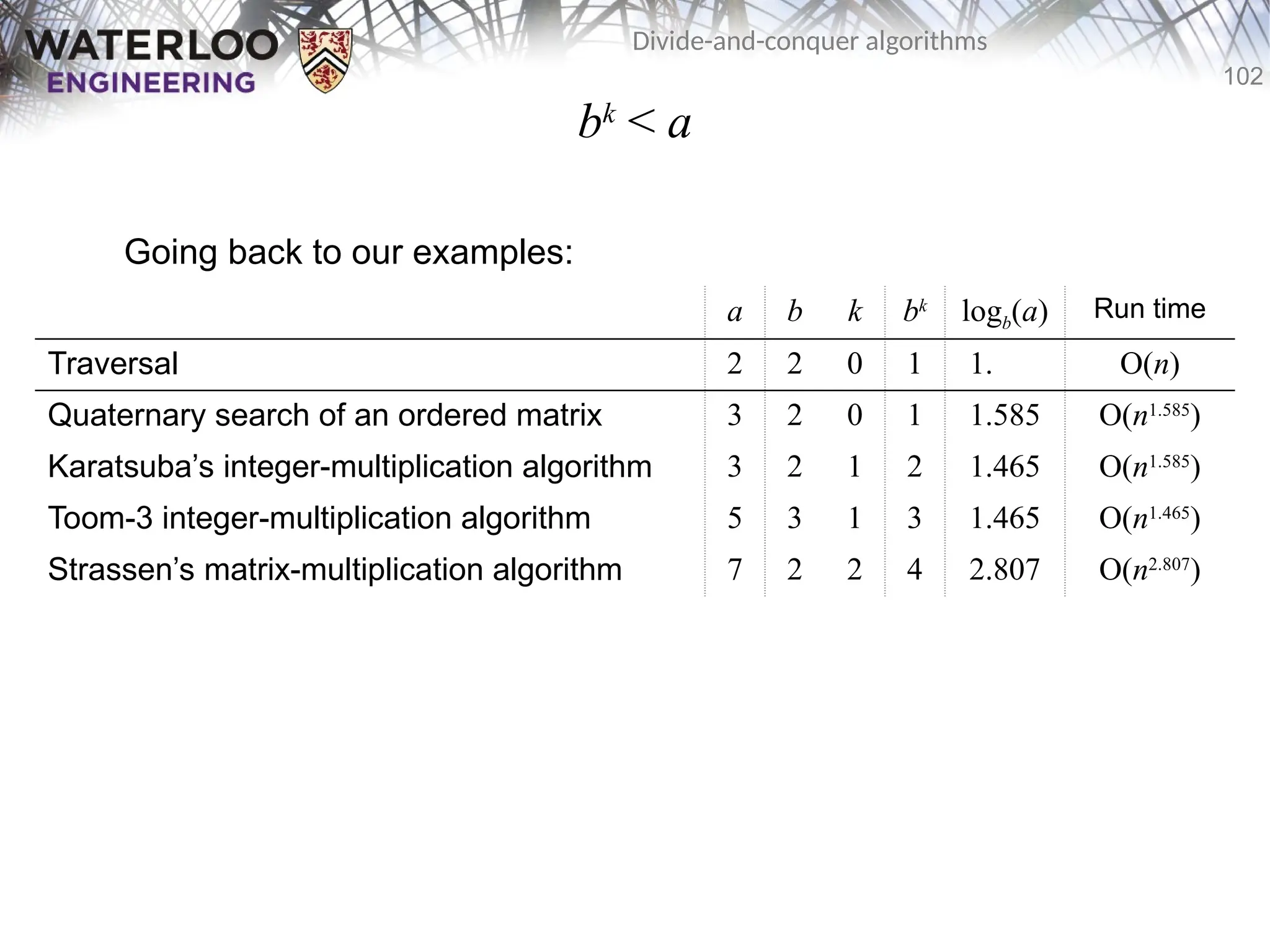
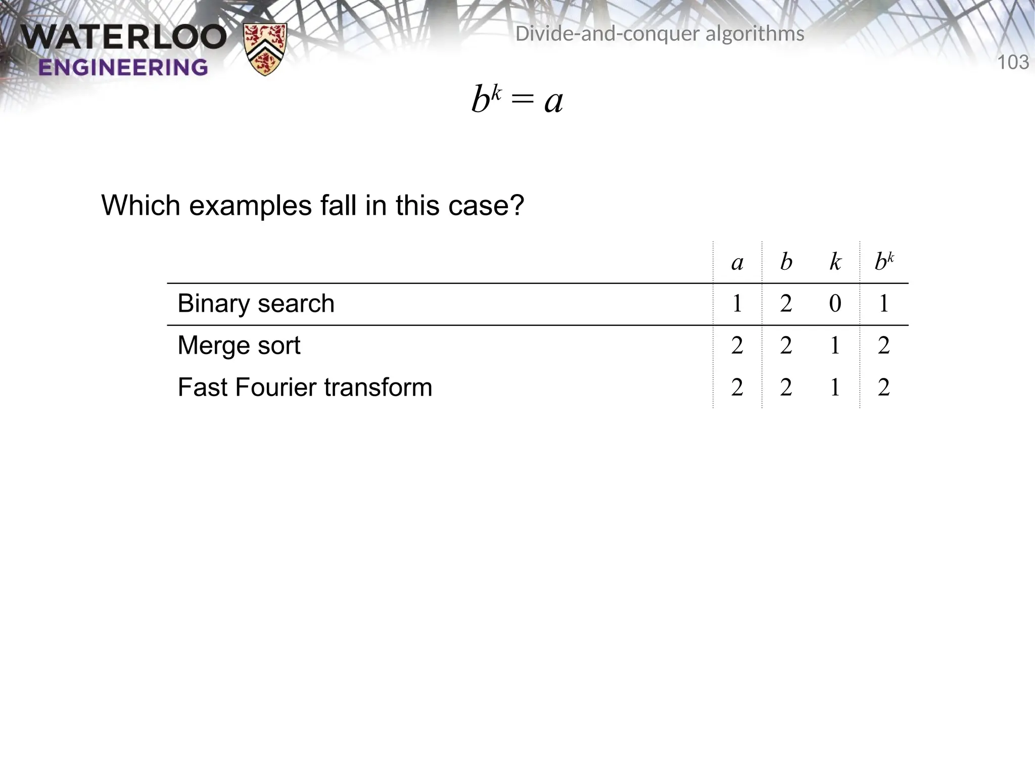
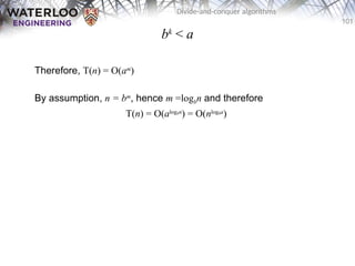
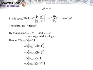
105.
105
Divide-and-conquer algorithms
bk
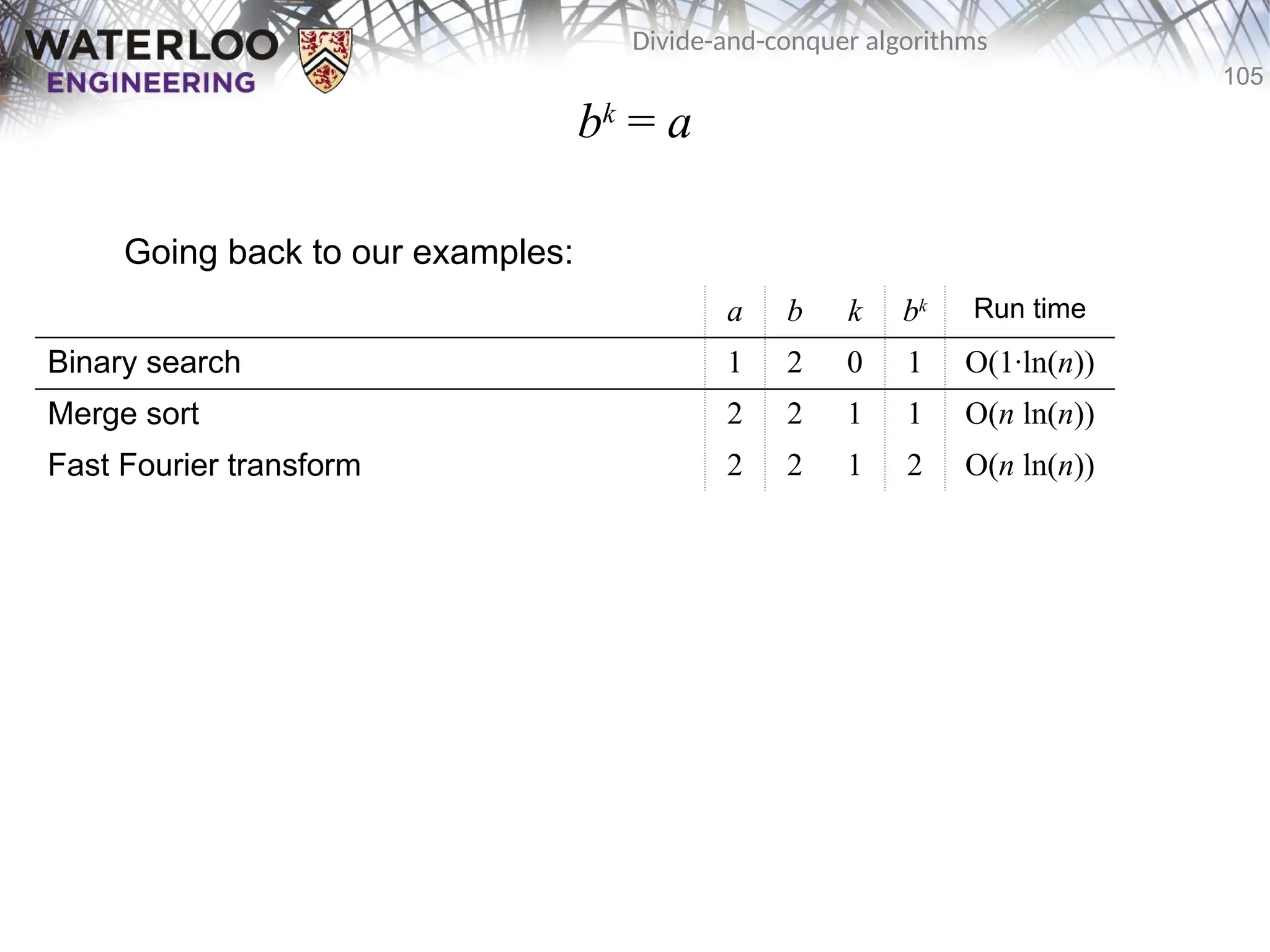
= a
Goingback to our examples:
a b k bk Run time
Binary search 1 2 0 1 O(1·ln(n))
Merge sort 2 2 1 1 O(n ln(n))
Fast Fourier transform 2 2 1 2 O(n ln(n))
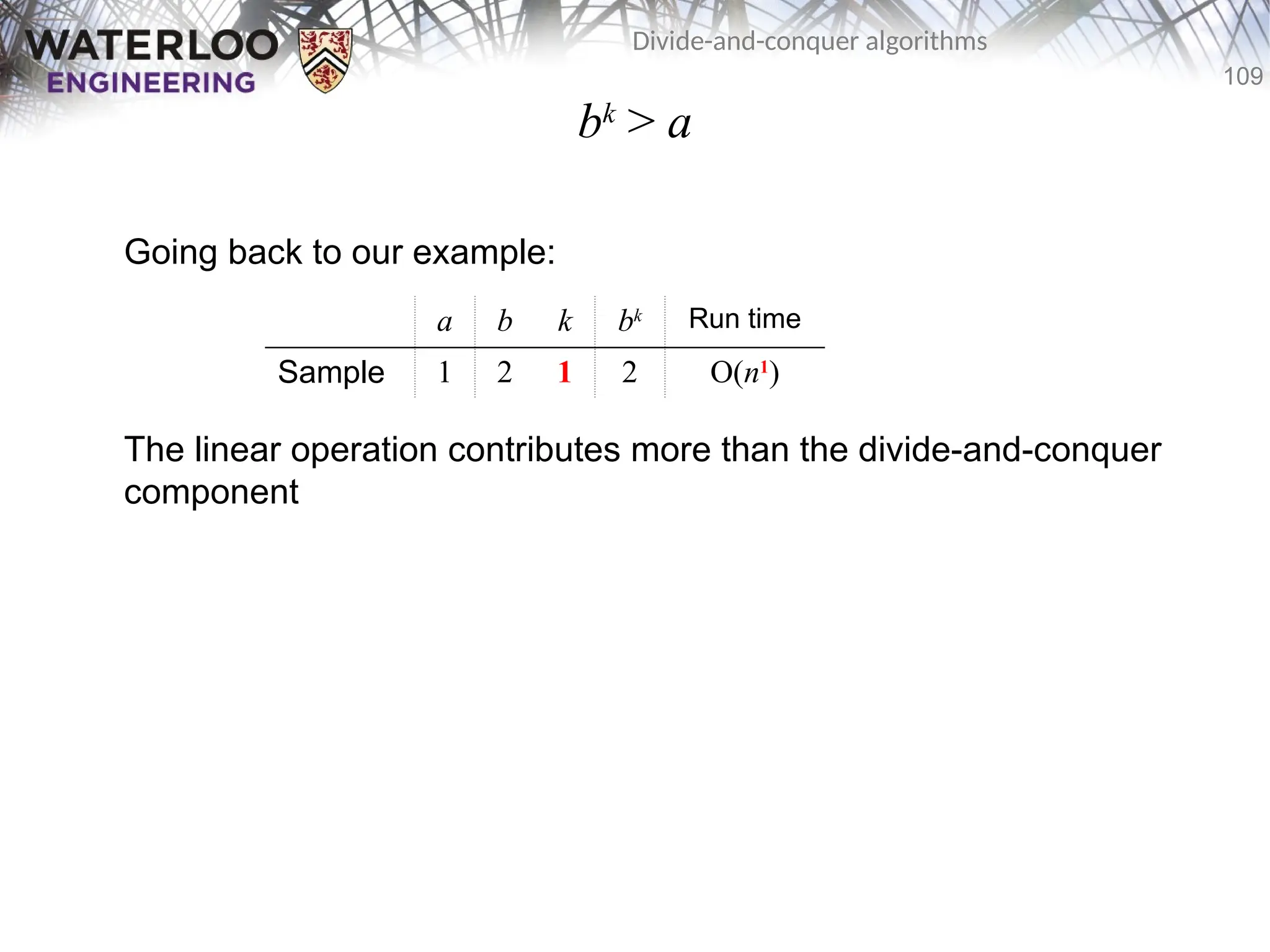
106.
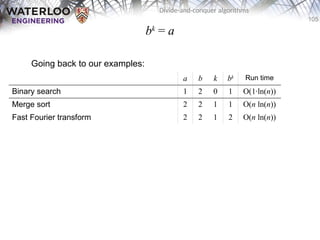
106
Divide-and-conquer algorithms
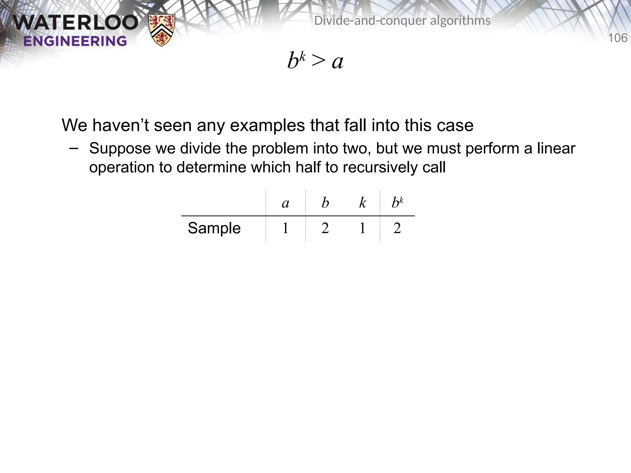
bk
> a
Wehaven’t seen any examples that fall into this case
– Suppose we divide the problem into two, but we must perform a linear
operation to determine which half to recursively call
a b k bk
Sample 1 2 1 2
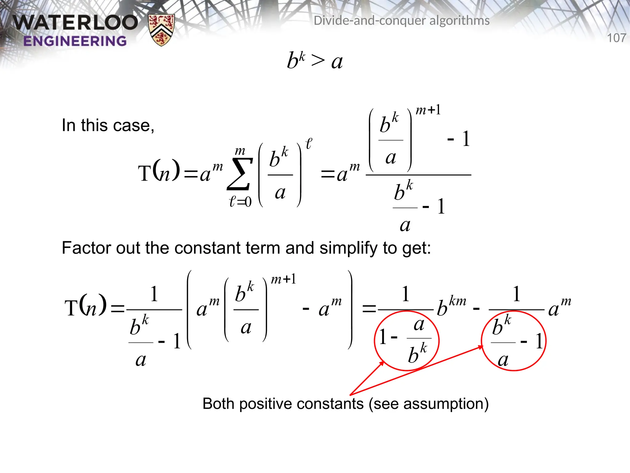
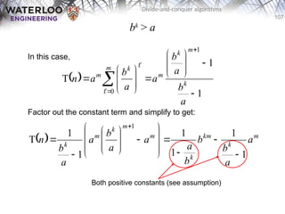
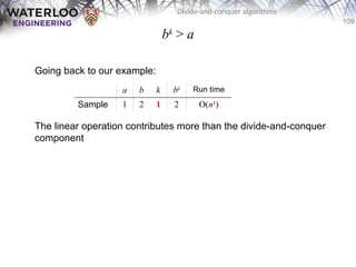
107.
107
Divide-and-conquer algorithms
bk
> a
Inthis case,
Factor out the constant term and simplify to get:
1
1
T
1
0
a
b
a
b
a
a
b
a
n k
m
k
m
m k
m
m
k
km
k
m
m
k
m
k
a
a
b
b
b
a
a
a
b
a
a
b
n
1
1
1
1
1
1
T
1
Both positive constants (see assumption)
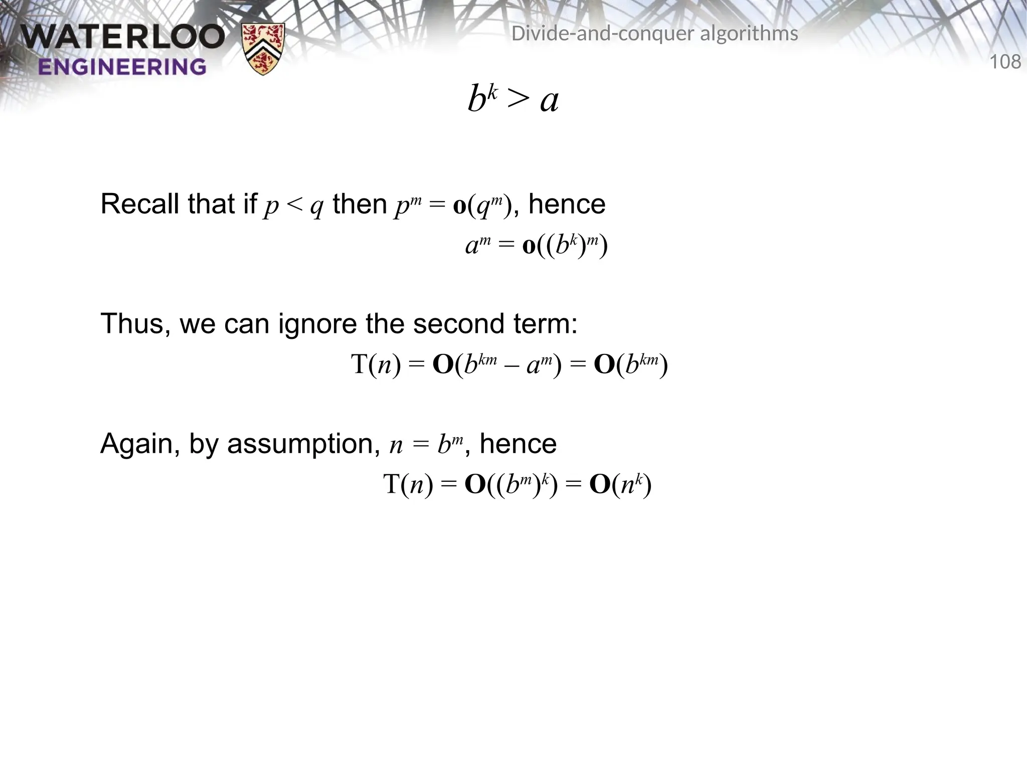
108.
108
Divide-and-conquer algorithms
bk
> a
Recallthat if p < q then pm
= o(qm
), hence
am
= o((bk
)m
)
Thus, we can ignore the second term:
T(n) = O(bkm
– am
) = O(bkm
)
Again, by assumption, n = bm
, hence
T(n) = O((bm
)k
) = O(nk
)
110
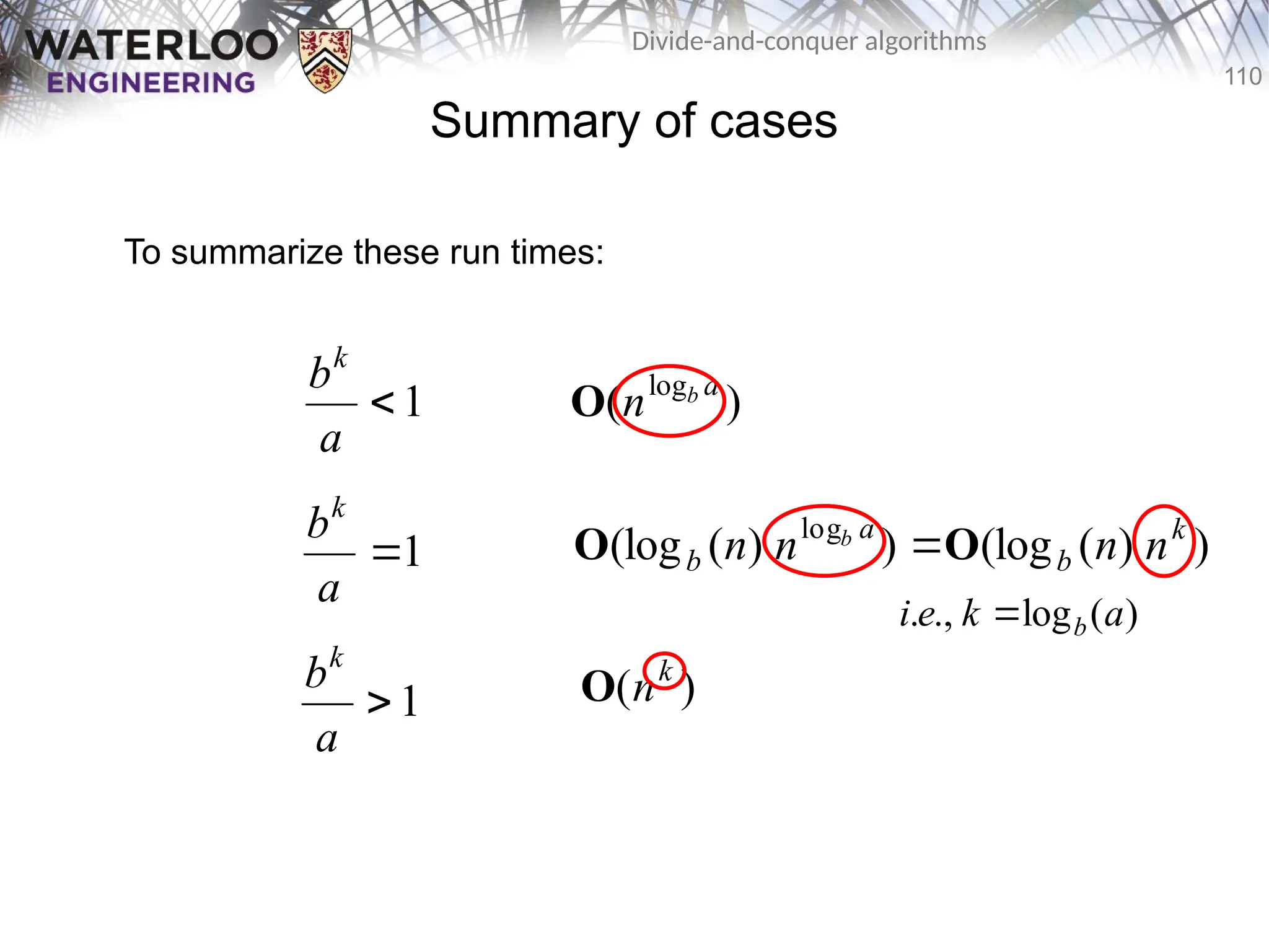
Divide-and-conquer algorithms
Summary ofcases
To summarize these run times:
1
a
bk
1
a
bk
1
a
bk
)
( log a
b
n
O
)
)
(
(log
)
)
(
(log log k
b
a
b n
n
n
n b
O
O
)
( k
n
O
)
(
log
.,
. a
k
e
i b
111.
111
Divide-and-conquer algorithms
Summary
Therefore:
– Ifthe amount of work being done at each step to either sub-divide the
problem or to recombine the solutions dominates, then this is the run
time of the algorithm: O(nk
)
– If the problem is being divided into many small sub-problems (a > bk
)
then the number of sub-problems dominates: O(nlogb(a)
)
– In between, a little more (logarithmically more) work must be done
112.
112
Divide-and-conquer algorithms
References
Wikipedia, http://en.wikipedia.org/wiki/Divide_and_conquer
Theseslides are provided for the ECE 250 Algorithms and Data Structures course. The
material in it reflects Douglas W. Harder’s best judgment in light of the information available to
him at the time of preparation. Any reliance on these course slides by any party for any other
purpose are the responsibility of such parties. Douglas W. Harder accepts no responsibility for
damages, if any, suffered by any party as a result of decisions made or actions based on these
course slides for any other purpose than that for which it was intended.


 );
1
)
1
(
2
T
3
1
1
)
T( n
n
n
n Θ
3
2
n
( )
log2 3 1
2
1.584962501](https://image.slidesharecdn.com/12-250806161017-fa62979a/85/12-03-Divide-and-conquer_algorithms-pptx-18-320.jpg)


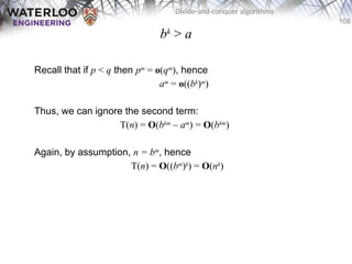
![81
Divide-and-conquer algorithms
Fast Fourier transform
void FFT( std::complex<double> *array, int n ) {
if ( n == 1 ) return;
std::complex<double> even[n/2];
std::complex<double> odd[n/2];
for ( int k = 0; k < n/2; ++k ) {
even[k] = array[2*k];
odd[k] = array[2*k + 1];
}
FFT( even, n/2 );
FFT( odd, n/2 );
double const PI = 4.0*std::atan( 1.0 );
std::complex<double> w = 1.0;
std::complex<double> wn = std::exp( std::complex<double>( 0.0, -2.0*PI/n ) );
for ( int k = 0; k < n/2; ++k ) {
array[k] = even[k] + w*odd[k];
array[n/2 + k] = even[k] - w*odd[k];
w = w * wn;
}
}
( )
n
( )
n
(1)
2
T
2 n
(1)
(1)
](https://image.slidesharecdn.com/12-250806161017-fa62979a/85/12-03-Divide-and-conquer_algorithms-pptx-81-320.jpg)

 );
1
)
1
(
2
T
3
1
1
)
T( n
n
n
n Θ
3
2
n
( )
log2 3 1
2
1.584962501](https://image.slidesharecdn.com/12-250806161017-fa62979a/75/12-03-Divide-and-conquer_algorithms-pptx-18-2048.jpg)


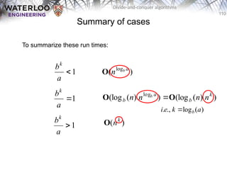
![81
Divide-and-conquer algorithms
Fast Fourier transform
void FFT( std::complex<double> *array, int n ) {
if ( n == 1 ) return;
std::complex<double> even[n/2];
std::complex<double> odd[n/2];
for ( int k = 0; k < n/2; ++k ) {
even[k] = array[2*k];
odd[k] = array[2*k + 1];
}
FFT( even, n/2 );
FFT( odd, n/2 );
double const PI = 4.0*std::atan( 1.0 );
std::complex<double> w = 1.0;
std::complex<double> wn = std::exp( std::complex<double>( 0.0, -2.0*PI/n ) );
for ( int k = 0; k < n/2; ++k ) {
array[k] = even[k] + w*odd[k];
array[n/2 + k] = even[k] - w*odd[k];
w = w * wn;
}
}
( )
n
( )
n
(1)
2
T
2 n
(1)
(1)
](https://image.slidesharecdn.com/12-250806161017-fa62979a/75/12-03-Divide-and-conquer_algorithms-pptx-81-2048.jpg)