22PCOAM16_MACHINE_LEARNING_UNIT_IV_NOTES_with_QB

22PCOAM16
MACHINE LEARNING
UNIT IV NOTES & QB
B.TECH
III YEAR – V SEM (R22)
(2024-2025)
Prepared
By
Dr. M.Gokilavani
Department of Emerging Technologies
(Special Batch)

UNIT-IV
Dimensionality Reduction – Linear Discriminate Analysis – Principal Component Analysis –
Factor Analysis – Independent Component Analysis – Locally Linear Embedding – Isomap –
Least Squares Optimization Evolutionary Learning – Genetic algorithms – Genetic Offspring: -
Genetic Operators – Using Genetic Algorithms.
I. DIMENSIONALITY REDUCTION:
 When working with machine learning models, datasets with too many features can cause
issues like slow computation and over fitting.
 Dimensionality reduction helps by reducing the number of features while retaining key
information.
 Techniques like
i. principal component analysis (PCA)
ii. singular value decomposition (SVD)
iii. linear discriminant analysis (LDA)
Project data onto a lower-dimensional space, preserving important details.
Example:
 When you are building a model to predict house prices with features like bedrooms, square
footage, and location. If you add too many features, such as room condition or flooring type,
the dataset becomes large and complex.
 Before Dimensionality Reduction:
o With too many features, training can slow down and the model may focus on irrelevant
details, like flooring type, which could lead to inaccurate predictions.
How Dimensionality Reduction Works?
 Lets understand how dimensionality Reduction is used with the help of the figure below:
Fig: Dimensionality Reduction
 On the left, data points exist in a 3D space (X, Y, Z), but the Z-dimension appears unnecessary
since the data primarily varies along the X and Y axes.

 The goal of dimensionality reduction is to remove less important dimensions without losing
valuable information.
 On the right, after reducing the dimensionality, the data is represented in lower-dimensional
spaces. The top plot (X-Y) maintains the meaningful structure, while the bottom plot (Z-Y)
shows that the Z-dimension contributed little useful information.
 This process makes data analysis more efficient, improving computation speed and visualization
while minimizing redundancy.
DIMENSIONALITY REDUCTION TECHNIQUES:
 Dimensionality reduction techniques can be broadly divided into two categories:
i. Feature Selection
ii. Feature Extraction
i. Feature selection:
 Chooses the most relevant features from the dataset without altering them. It helps
remove redundant or irrelevant features, improving model efficiency.
 There are several methods for feature selection including filter methods, wrapper
methods and embedded methods.
 Filter methods rank the features based on their relevance to the target variable.
 Wrapper methods use the model performance as the criteria for selecting features.
 Embedded methods combine feature selection with the model training process.
ii. Feature Extraction
 Feature extraction involves creating new features by combining or transforming the
original features.
 There are several methods for feature extraction stated above in the introductory part
which is responsible for creating and transforming the features.
 PCA is a popular technique that projects the original features onto a lower-dimensional
space while preserving as much of the variance as possible.
Dimensionality reduction with several techniques:
 Principal Component Analysis (PCA): Converts correlated variables into uncorrelated
‘principal components,’ reducing dimensionality while maintaining as much variance as
possible, enabling more efficient analysis.
 Missing Value Ratio: Variables with missing data beyond a set threshold are removed,
improving dataset reliability.
 Backward Feature Elimination: Starts with all features and removes the least significant
ones in each iteration. The process continues until only the most impactful features remain,
optimizing model performance.
 Forward Feature Selection: Forward Feature Selection Begins with one feature, adds others
incrementally, and keeps that improving model performance.
 Random Forest: Random forest Uses decision trees to evaluate feature importance,
automatically selecting the most relevant features without the need for manual coding,
enhancing model accuracy.

 Factor Analysis: Groups variables by correlation and keeps the most relevant ones for further
analysis.
 Independent Component Analysis (ICA): Identifies statistically independent components,
ideal for applications like ‘blind source separation’ where traditional correlation-based
methods fall short.
Dimensionality Reduction Examples:
 Dimensionality reduction plays a crucial role in many real-world applications, such as text
categorization, image retrieval, gene expression analysis, and more. Here are a few examples:
1. Text Categorization: With vast amounts of online data, dimensionality reduction helps
classify text documents into predefined categories by reducing the feature space (like
word or phrase features) while maintaining accuracy.
2. Image Retrieval: As image data grows, indexing based on visual content (color, texture,
shape) rather than just text descriptions has become essential. This allows for better
retrieval of images from large databases.
3. Gene Expression Analysis: Dimensionality reduction accelerates gene expression
analysis, helping classify samples (e.g., leukemia) by identifying key features,
improving both speed and accuracy.
4. Intrusion Detection: In cyber security, dimensionality reduction helps analyze user
activity patterns to detect suspicious behaviors and intrusions by identifying optimal
features for network monitoring.
Advantages of Dimensionality Reduction:
 Faster Computation: With fewer features, machine learning algorithms can process data
more quickly. This results in faster model training and testing, which is particularly useful
when working with large datasets.
 Better Visualization: As we saw in the earlier figure, reducing dimensions makes it easier to
visualize data, revealing hidden patterns.
 Prevent Over fitting: With fewer features, models are less likely to memorize the training
data and over fit. This helps the model generalize better to new, unseen data, improving its
ability to make accurate predictions.
Disadvantages of Dimensionality Reduction:
 Data Loss & Reduced Accuracy – Some important information may be lost during
dimensionality reduction, potentially affecting model performance.
 Choosing the Right Components – Deciding how many dimensions to keep is difficult, as
keeping too few may lose valuable information, while keeping too many can lead to over
fitting.
II. LINEAR DISCRIMINATEANALYSIS:
 When working with high-dimensional datasets it is important to apply dimensionality
reduction techniques to make data exploration and modeling more efficient.
 One such technique is Linear Discriminate Analysis (LDA) which helps in reducing the
dimensionality of data while retaining the most significant features for classification tasks.
 It works by finding the linear combinations of features that best separate the classes in the
dataset.

Role of LDA:
 Linear Discriminate Analysis (LDA) also known as Normal Discriminate Analysis is
supervised classification problem that helps separate two or more classes by converting
higher-dimensional data space into a lower-dimensional space.
 It is used to identify a linear combination of features that best separates classes within a
dataset.
Fig: Overlapping LDA
 For example we have two classes that need to be separated efficiently.
 Each class may have multiple features and using a single feature to classify them may result
in overlapping. To solve this LDA is used as it uses multiple features to improve
classification accuracy.
 LDA works by some assumptions and we are required to understand them so that we have a
better understanding of its working.
Implementation of LDA:
For LDA to perform effectively certain assumptions are made:
1. Gaussian distribution: Data within each class should follow a Gaussian distribution.
2. Equal Covariance Matrices: Covariance matrices of the different classes should be
equal.
3. Linear Separability: A linear decision boundary should be sufficient to separate the
classes.
Example: when data points belonging to two classes are plotted if they are not linearly separable
LDA will attempt to find a projection that maximizes class separability.

 LDA attempts to separate them using red dashed line.
 It uses both axes (X and Y) to generate a new axis in such a way that it maximizes the
distance between the means of the two classes while minimizing the variation within each
class.
 This transforms the dataset into a space where the classes are better separated.
 After transforming the data points along a new axis LDA maximizes the class separation.
 This new axis allows for clearer classification by projecting the data along a line that
enhances the distance between the means of the two classes.
 Perpendicular distance between the decision boundary and the data points helps us to
visualize how LDA works by reducing class variation and increasing separability.
 After generating this new axis using the above-mentioned criteria, all the data points of the
classes are plotted on this new axis and are shown in the figure given below.
Working of LDA:
 LDA works by finding directions in the feature space that best separate the classes. It does
this by maximizing the difference between the class means while minimizing the spread
within each class.
Step 1: Compute the mean vectors for each class.
Step 2: Calculate the within-class and between-class scatter matrices.
Step 3: Solve for the linear discriminants that maximize the ratio of between-class
variance to within-class variance.
Step 4: Project the data onto the new lower-dimensional space.
Advantages of LDA:
 Simple and computationally efficient.
 Works well even when the number of features is much larger than the number of training
samples.
 Can handle multicollinearity.
Disadvantages of LDA:
 Assumes Gaussian distribution of data which may not always be the case.
 Assumes equal covariance matrices for different classes which may not hold in all datasets.
 Assumes linear separability which is not always true.
 May not always perform well in high-dimensional feature spaces.
Applications of LDA:
1. Face Recognition: It is used to reduce the high-dimensional feature space of pixel values in
face recognition applications helping to identify faces more efficiently.
2. Medical Diagnosis: It classifies disease severity in mild, moderate or severe based on
patient parameters helping in decision-making for treatment.
3. Customer Identification: It can help identify customer segments most likely to purchase a
specific product based on survey data.
III. PRINCIPAL COMPONENT ANALYSIS:
 Principal component analysis is a useful statistical technique that has found applications in
diverse fields. It helps in reducing the dimensionality of the data set and identification of patterns
in the data through graphical representation.
 PCA is simple: reduce the number of variables of a data set, while preserving as much
information as possible.

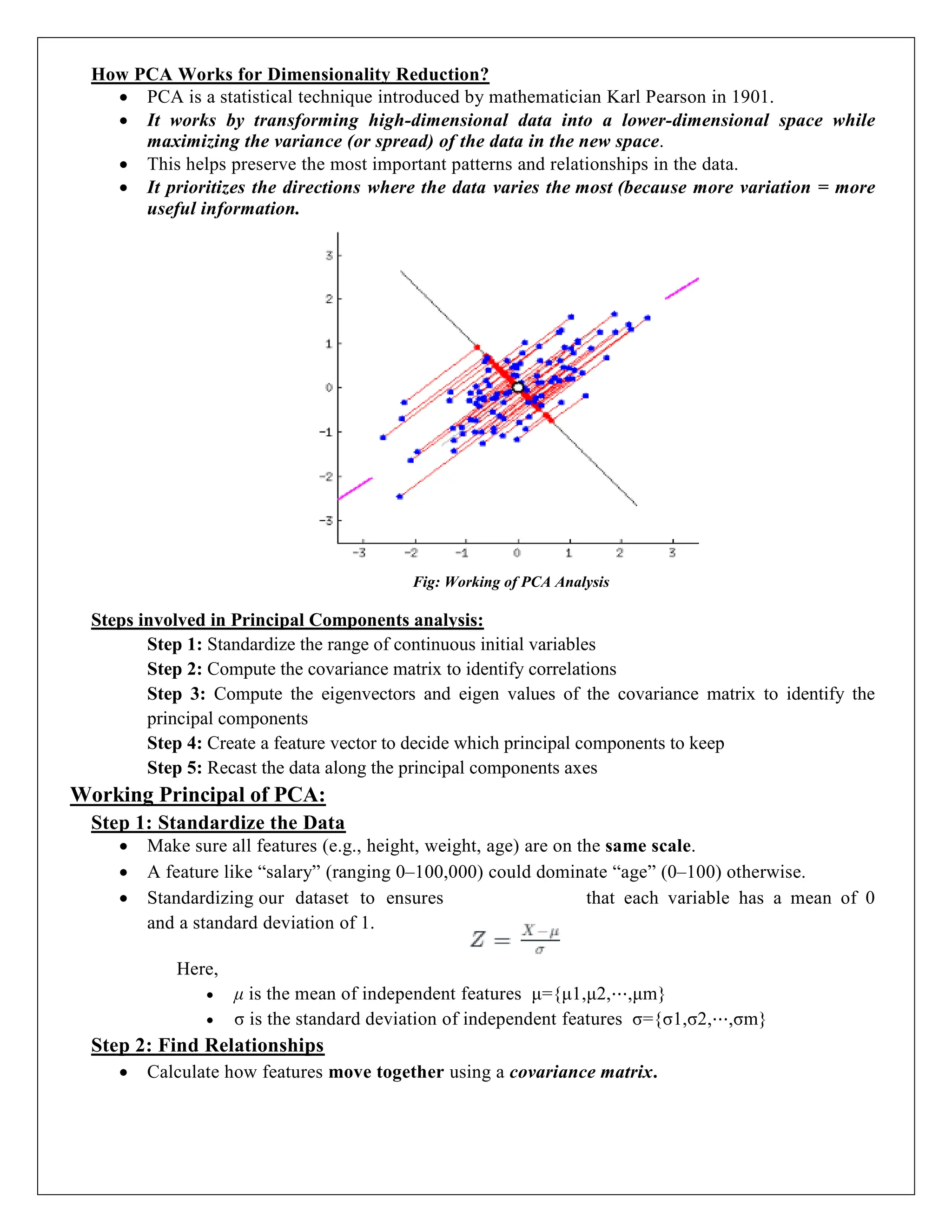
How PCA Works for Dimensionality Reduction?
 PCA is a statistical technique introduced by mathematician Karl Pearson in 1901.
 It works by transforming high-dimensional data into a lower-dimensional space while
maximizing the variance (or spread) of the data in the new space.
 This helps preserve the most important patterns and relationships in the data.
 It prioritizes the directions where the data varies the most (because more variation = more
useful information.
Fig: Working of PCA Analysis
Steps involved in Principal Components analysis:
Step 1: Standardize the range of continuous initial variables
Step 2: Compute the covariance matrix to identify correlations
Step 3: Compute the eigenvectors and eigen values of the covariance matrix to identify the
principal components
Step 4: Create a feature vector to decide which principal components to keep
Step 5: Recast the data along the principal components axes
Working Principal of PCA:
Step 1: Standardize the Data
 Make sure all features (e.g., height, weight, age) are on the same scale.
 A feature like “salary” (ranging 0–100,000) could dominate “age” (0–100) otherwise.
 Standardizing our dataset to ensures that each variable has a mean of 0
and a standard deviation of 1.
Here,
 μ is the mean of independent features μ={μ1,μ2,⋯,μm}
 σ is the standard deviation of independent features σ={σ1,σ2,⋯,σm}
Step 2: Find Relationships
 Calculate how features move together using a covariance matrix.

 Covariance measures the strength of joint variability between two or more variables,
indicating how much they change in relation to each other.
 To find the covariance we can use the formula:
The value of covariance can be positive, negative, or zeros.
 Positive: As the x1 increases x2 also increases.
 Negative: As the x1 increases x2 also decreases.
 Zeros: No direct relation.
Step 3: Find the “Magic Directions” (Principal Components)
PCA identifies new axes (like rotating a camera) where the data spreads out the most:
o 1st Principal Component (PC1): The direction of maximum variance (most spread).
o 2nd Principal Component (PC2): The next best direction, perpendicular to PC1, and
so on.
 These directions are calculated using Eigenvalues and Eigenvectors
Where:
o Eigenvectors (math tools that find these axes), and their importance is ranked
o Eigenvalues (how much variance each captures).
For a square matrix A, an eigenvector X (a non-zero vector) and its corresponding eigenvalues
λ (a scalar) satisfy:
This means:
 When A acts on X, it only stretches or shrinks X by the scalar λ.
 The direction of X remains unchanged (hence, eigenvectors define “stable directions” of A).
It can also be written as:
Where I is the identity matrix of the same shape as matrix A. And the above conditions will be true
only if (A–λI) will be non-invertible (i.e. singular matrix). That means,
∣A–λI∣=0
This determinant equation is called the characteristic equation.
 Solving it gives the eigenvalues lambda,
 Therefore corresponding eigenvector can be found using the equation AX=λX.
Step 4: Pick the Top Directions & Transform Data
 Keep only the top 2–3 directions (or enough to capture ~95% of the variance).
 Project the data onto these directions to get a simplified, lower-dimensional version.
 PCA is an unsupervised learning algorithm, meaning it doesn’t require prior knowledge of
target variables. It’s commonly used in exploratory data analysis and machine learning
to simplify datasets without losing critical information.

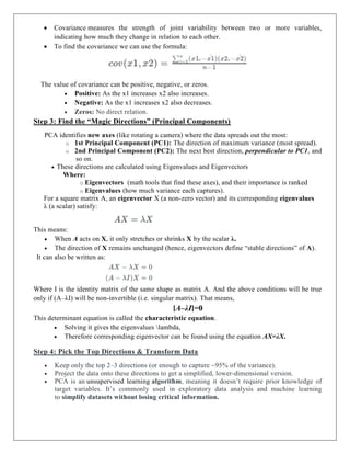
Fig: Transform this 2D dataset into a 1D representation while preserving as much variance as possible.
Principal Components (PCs):
 PC₁ (First Principal Component): The direction along which the data has the maximum
variance. It captures the most important information.
 PC₂ (Second Principal Component): The direction orthogonal (perpendicular) to PC₁. It
captures the remaining variance but is less significant.
 The red dashed lines indicate the spread (variance) of data along different directions. The
variance along PC₁ is greater than PC₂, which means that PC₁ carries more useful
information about the dataset.
 The data points (blue dots) are projected onto PC₁, effectively reducing the dataset from
two dimensions (Radius, Area) to one dimension (PC₁).
 This transformation simplifies the dataset while retaining most of the original variability.
Advantages of Principal Component Analysis:
1. Multicollinearity Handling: Creates new, uncorrelated variables to address issues when
original features are highly correlated.
2. Noise Reduction: Eliminates components with low variance (assumed to be noise),
enhancing data clarity.
3. Data Compression: Represents data with fewer components, reducing storage needs and
speeding up processing.
4. Outlier Detection: Identifies unusual data points by showing which ones deviate
significantly in the reduced space.
Disadvantages of Principal Component Analysis:
1. Interpretation Challenges: The new components are combinations of original variables,
which can be hard to explain.

2. Data Scaling Sensitivity: Requires proper scaling of data before application, or results may
be misleading.
3. Information Loss: Reducing dimensions may lose some important information if too few
components are kept.
4. Assumption of Linearity: Works best when relationships between variables are linear, and
may struggle with non-linear data.
5. Computational Complexity: Can be slow and resource-intensive on very large datasets.
6. Risk of over fitting: Using too many components or working with a small dataset might lead
to models that don’t generalize well.
IV. FACTOR ANALYSIS:
 Factor analysis is a statistical method used to analyze the relationships among a set of
observed variables by explaining the correlations or covariance’s between them in terms of
a smaller number of unobserved variables called factors.
 Factor analysis, a method within the realm of statistics and part of the general linear model
(GLM), serves to condense numerous variables into a smaller set of factors.
 Factor analysis operates under several assumptions: linearity in relationships, absence of
multicollinearity among variables, inclusion of relevant variables in the analysis, and
genuine correlations between variables and factors.
What does Factor mean in Factor Analysis?
 Factor analysis, a “factor” refers to an underlying, unobserved variable or latent construct that
represents a common source of variation among a set of observed variables.
 These observed variables, also known as indicators or manifest variables, are the measurable
variables that are directly observed or measured in a study.
How to do Factor Analysis (Factor Analysis Steps)?
 Factor analysis is a statistical method used to describe variability among observed, correlated
variables in terms of a potentially lower number of unobserved variables called factors. Here
are the general steps involved in conducting a factor analysis:
Step 1. Determine the Suitability of Data for Factor Analysis
 Bartlett’s Test: Check the significance level to determine if the correlation matrix is
suitable for factor analysis.
 Kaiser-Meyer-Olkin (KMO) Measure: Verify the sampling adequacy. A value greater
than 0.6 is generally considered acceptable.
Step 2. Choose the Extraction Method
 Principal Component Analysis (PCA): Used when the main goal is data reduction.
 Principal Axis Factoring (PAF): Used when the main goal is to identify underlying
factors.
Step 3. Factor Extraction
 Use the chosen extraction method to identify the initial factors.
 Extract eigenvalues to determine the number of factors to retain. Factors with
eigenvalues greater than 1 are typically retained in the analysis.
 Compute the initial factor loadings.

Step 4. Determine the Number of Factors to Retain
 Scree Plot: Plot the eigenvalues in descending order to visualize the point where the
plot levels off (the “elbow”) to determine the number of factors to retain.
 Eigenvalues: Retain factors with eigenvalues greater than 1.
Step 5. Factor Rotation
 Orthogonal Rotation (Varimax, Quartimax): Assumes that the factors are
uncorrelated.
 Oblique Rotation (Promax, Oblimin): Allows the factors to be correlated.
 Rotate the factors to achieve a simpler and more interpretable factor structure.
 Examine the rotated factor loadings.
Step 6. Interpret and Label the Factors
 Analyze the rotated factor loadings to interpret the underlying meaning of each factor.
 Assign meaningful labels to each factor based on the variables with high loadings on
that factor.
Step 7. Compute Factor Scores (if needed)
 Calculate the factor scores for each individual to represent their value on each factor.
Step 8. Report and Validate the Results
 Report the final factor structure, including factor loadings and communalities.
 Validate the results using additional data or by conducting a confirmatory factor
analysis if necessary.
Why do we need Factor Analysis?
Factorial analysis serves several purposes and objectives in statistical analysis:
1. Dimensionality Reduction: Factor analysis helps in reducing the number of variables under
consideration by identifying a smaller number of underlying factors that explain the correlations
or covariance’s among the observed variables. This simplification can make the data more
manageable and easier to interpret.
2. Identifying Latent Constructs: It allows researchers to identify latent constructs or underlying
factors that may not be directly observable but are inferred from patterns in the observed data.
These latent constructs can represent theoretical concepts, such as personality traits, attitudes, or
socioeconomic status.
3. Data Summarization: By condensing the information from multiple variables into a smaller set
of factors, factor analysis provides a more concise summary of the data while retaining as much
relevant information as possible.
4. Hypothesis Testing: Factor analysis can be used to test hypotheses about the underlying
structure of the data. For example, researchers may have theoretical expectations about how
variables should be related to each other, and factor analysis can help evaluate whether these
expectations are supported by the data.
5. Variable Selection: It aids in identifying which variables are most important or relevant for
explaining the underlying factors. This can help in prioritizing variables for further analysis or
for developing more parsimonious models.

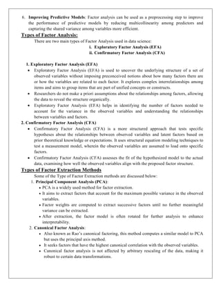
6. Improving Predictive Models: Factor analysis can be used as a preprocessing step to improve
the performance of predictive models by reducing multicollinearity among predictors and
capturing the shared variance among variables more efficient.
Types of Factor Analysis:
There are two main types of Factor Analysis used in data science:
i. Exploratory Factor Analysis (EFA)
ii. Confirmatory Factor Analysis (CFA)
1. Exploratory Factor Analysis (EFA)
 Exploratory Factor Analysis (EFA) is used to uncover the underlying structure of a set of
observed variables without imposing preconceived notions about how many factors there are
or how the variables are related to each factor. It explores complex interrelationships among
items and aims to group items that are part of unified concepts or constructs.
 Researchers do not make a priori assumptions about the relationships among factors, allowing
the data to reveal the structure organically.
 Exploratory Factor Analysis (EFA) helps in identifying the number of factors needed to
account for the variance in the observed variables and understanding the relationships
between variables and factors.
2. Confirmatory Factor Analysis (CFA)
 Confirmatory Factor Analysis (CFA) is a more structured approach that tests specific
hypotheses about the relationships between observed variables and latent factors based on
prior theoretical knowledge or expectations. It uses structural equation modeling techniques to
test a measurement model, wherein the observed variables are assumed to load onto specific
factors.
 Confirmatory Factor Analysis (CFA) assesses the fit of the hypothesized model to the actual
data, examining how well the observed variables align with the proposed factor structure.
Types of Factor Extraction Methods
Some of the Type of Factor Extraction methods are discussed below:
1. Principal Component Analysis (PCA):
 PCA is a widely used method for factor extraction.
 It aims to extract factors that account for the maximum possible variance in the observed
variables.
 Factor weights are computed to extract successive factors until no further meaningful
variance can be extracted.
 After extraction, the factor model is often rotated for further analysis to enhance
interpretability.
2. Canonical Factor Analysis:
 Also known as Rao’s canonical factoring, this method computes a similar model to PCA
but uses the principal axis method.
 It seeks factors that have the highest canonical correlation with the observed variables.
 Canonical factor analysis is not affected by arbitrary rescaling of the data, making it
robust to certain data transformations.

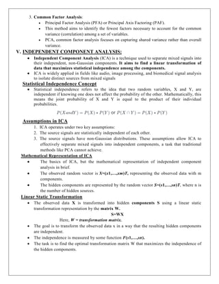
3. Common Factor Analysis:
 Principal Factor Analysis (PFA) or Principal Axis Factoring (PAF).
 This method aims to identify the fewest factors necessary to account for the common
variance (correlation) among a set of variables.
 PCA, common factor analysis focuses on capturing shared variance rather than overall
variance.
V. INDEPENDENT COMPONENT ANALYSIS:
 Independent Component Analysis (ICA) is a technique used to separate mixed signals into
their independent, non-Gaussian components. It aims to find a linear transformation of
data that maximizes statistical independence among the components.
 ICA is widely applied in fields like audio, image processing, and biomedical signal analysis
to isolate distinct sources from mixed signals
Statistical Independence Concept
 Statistical independence refers to the idea that two random variables, X and Y, are
independent if knowing one does not affect the probability of the other. Mathematically, this
means the joint probability of X and Y is equal to the product of their individual
probabilities.
Assumptions in ICA
1. ICA operates under two key assumptions:
2. The source signals are statistically independent of each other.
3. The source signals have non-Gaussian distributions. These assumptions allow ICA to
effectively separate mixed signals into independent components, a task that traditional
methods like PCA cannot achieve.
Mathematical Representation of ICA
 The basics of ICA, but the mathematical representation of independent component
analysis in brief.
 The observed random vector is X=(x1,…,xm)T, representing the observed data with m
components.
 The hidden components are represented by the random vector S=(s1,…,sn)T, where n is
the number of hidden sources.
Linear Static Transformation
 The observed data X is transformed into hidden components S using a linear static
transformation representation by the matrix W.
S=WX
Here, W = transformation matrix.
 The goal is to transform the observed data x in a way that the resulting hidden components
are independent.
 The independence is measured by some function F(s1,…,sn).
 The task is to find the optimal transformation matrix W that maximizes the independence of
the hidden components.

Implementing of ICA:
 Implementation of the Independent Component Analysis (ICA) algorithm that is designed for
efficiency and speed.
Step 1: Import necessary libraries
Step 2: Generate Random Data and Mix the Signals
In the following code snippet,
 Random seed is set to generate random numbers.
 Samples and Time parameters are defined.
 Synthetic signals are generated and then combined to single matrix “S”.
 Noise is added to each element of the matrix.
 Matrix “A” is defined with coefficients the represent how the original signals are combined to
form observed signals.
 The observed signals are obtained by multiplying the matrix “S” by the transpose of the mixing
matrix “A”.
Step 3: Apply ICA to unmix the signals
In the following code snippet,
 An instance of FastICA class is created and number of independent components is set to 3.
 Fast ICA algorithm is applied to the observed mixed signals ‘X’. This fits the model to the
data and transforms the data to obtain the estimated independent sources (S_).
Step 4: Visualize the signals
Advantages of Independent Component Analysis (ICA):
 ICA is a powerful tool for separating mixed signals into their independent components. This is
useful in a variety of applications, such as signal processing, image analysis, and data
compression.
 ICA is a non-parametric approach, which means that it does not require assumptions about the
underlying probability distribution of the data.
 ICA is an unsupervised learning technique, which means that it can be applied to data without
the need for labeled examples. This makes it useful in situations where labeled data is not
available.
 ICA can be used for feature extraction, which means that it can identify important features in
the data that can be used for other tasks, such as classification.
Disadvantages of Independent Component Analysis (ICA):
 ICA assumes that the underlying sources are non-Gaussian, which may not always be true. If the
underlying sources are Gaussian, ICA may not be effective.
 ICA assumes that the sources are mixed linearly, which may not always be the case. If the
sources are mixed nonlinearly, ICA may not be effective.
 ICA can be computationally expensive, especially for large datasets. This can make it difficult
to apply ICA to real-world problems.
 ICA can suffer from convergence issues, which means that it may not always be able to find a
solution. This can be a problem for complex datasets with many sources.

VI. LOCALLY LINEAR EMBEDDING:
 LLE (Locally Linear Embedding) is an unsupervised approach designed to transform data
from its original high-dimensional space into a lower-dimensional representation, all while
striving to retain the essential geometric characteristics of the underlying non-linear feature
structure.
Steps in LLE operate:
oStep 1: It constructs a nearest neighbors graph to capture these local relationships.
 Then, it optimizes weight values for each data point, aiming to minimize the
reconstruction error when expressing a point as a linear combination of its
neighbors.
 This weight matrix reflects the strength of connections between points.
oStep 2: LLE computes a lower dimensional representation of the data by
finding eigenvectors of a matrix derived from the weight matrix.
 These eigenvectors represent the most relevant directions in the reduced space.
 Users can specify the desired dimensionality for the output space, and LLE
selects the top eigenvectors accordingly.
Mathematical Implementation of LLE Algorithm:
 The key idea of LLE is that locally, in the vicinity of each data point, the data lies
approximately on a linear subspace.
 LLE attempts to unfold or unroll the data while preserving these local linear relationships.
Here is a mathematical overview of the LLE algorithm:
Where:
 xi represents the i-th data point.
 wij are the weights that minimize the reconstruction error for data point xi using its
neighbors.
Locally Linear Embedding Algorithm:
The LLE algorithm can be broken down into several steps:
 Neighborhood Selection: For each data point in the high-dimensional space, LLE identifies
its k-nearest neighbors. This step is crucial because LLE assumes that each data point can be
well approximated by a linear combination of its neighbors.
 Weight Matrix Construction: LLE computes a set of weights for each data point to express
it as a linear combination of its neighbors. These weights are determined in such a way that
the reconstruction error is minimized. Linear regression is often used to find these weights.
 Global Structure Preservation: After constructing the weight matrix, LLE aims to find a
lower-dimensional representation of the data that best preserves the local linear relationships.
It does this by seeking a set of coordinates in the lower-dimensional space for each data point
that minimizes a cost function. This cost function evaluates how well each data point can be
represented by its neighbors.

 Output Embedding: Once the optimization process is complete, LLE provides the final
lower-dimensional representation of the data. This representation captures the essential
structure of the data while reducing its dimensionality.
Parameters in LLE Algorithm:
LLE has a few parameters that influence its behavior:
 k (Number of Neighbors): Explain how to select the optimal number of neighbors,
balancing local and global relationships.
 Dimensionality of Output Space: Discuss the importance of choosing the right
dimensionality for the final representation.
 Distance Metric: Introduce different distance metrics like Euclidean or Manhattan and
explain their impact.
 Regularization: If applicable, briefly mention how regularization helps avoid over
fitting.
Advantages of LLE:
 Preservation of Local Structures: LLE is excellent at maintaining the in-data local
relationships or structures. It successfully captures the inherent geometry of nonlinear
manifolds by maintaining pair wise distances between nearby data points.
 Handling Non-Linearity: LLE has the ability to capture nonlinear patterns and structures
in the data, in contrast to linear techniques like Principal Component Analysis (PCA).
When working with complicated, curved, or twisted datasets, it is especially helpful.
 Dimensionality Reduction: LLE lowers the dimensionality of the data while preserving its
fundamental properties. Particularly when working with high-dimensional datasets, this
reduction makes data presentation, exploration, and analysis simpler.
Disadvantages of LLE:
 Curse of Dimensionality: LLE can experience the "curse of dimensionality" when used
with extremely high-dimensional data, just like many other dimensionality reduction
approaches. The number of neighbors required to capture local interactions rises as
dimensionality does, potentially increasing the computational cost of the approach.
 Memory and computational Requirements: For big datasets, creating a weighted
adjacency matrix as part of LLE might be memory-intensive. The eigenvalue decomposition
stage can also be computationally taxing for big datasets.
 Outliers and Noisy data: LLE is susceptible to anomalies and jittery data points. The
quality of the embedding may be affected and the local linear relationships may be distorted
by outliers.
VII. ISOMAP:
 Isomap (Isometric Mapping) is a powerful technique used in dimensionality
reduction designed to preserve the essential structure of high-dimensional data.
 Linear techniques like PCA (Principal Component Analysis), Isomap excels at
uncovering the non-linear relationships hidden within data, such as those found in
images, speech, or biological data.
 This makes it a valuable tool for machine learning tasks where traditional methods may
fall short.

Why Isomap?
 When working with complex, high-dimensional datasets, Isomap offers an advantage over
linear methods by capturing non-linear patterns.
 This ability to retain the geometry of data points in a lower-dimensional space allows for
better analysis, visualization, and interpretation of complex datasets.
Understanding Manifold Learning:
 To fully understand Isomap, it’s essential to grasp the concept of manifold learning, which is
the basis for this technique
 Manifold Learning is a form of unsupervised learning that aims to reveal the intrinsic
structure of high-dimensional data. It treats data as if it lies on a lower-dimensional
"manifold" embedded in a higher-dimensional space.
 Isomap is one such manifold learning technique that preserves the geometric relationships in
data as it reduces dimensions
Geodesic Distances and Euclidean Distances:
In manifold learning, we distinguish between two types of distances:
 Geodesic Distance is the shortest path between two points along the manifold’s surface,
taking into account its curvature.
 Euclidean Distance is the straight-line distance between two points in the original space.
Isomap focuses on preserving geodesic distances, which reflect the true geometry of the data,
unlike Euclidean distances, which may distort the relationships in non-linear datasets
The Concept of Isometric Mapping
 At the heart of Isomap is the idea of Isometric Mapping, which aims to preserve pair wise
distances between points.
 This ensures that the data’s internal structure is retained even as it is reduced to a lower-
dimensional representation.
 Isomap's goal is to ensure that the geodesic distances between points remain as accurate as
possible, even when simplifying the data.
Working of Isomap:
1. Step 01: Calculate Pairwise Distances: Begin by computing the Euclidean distances between
all pairs of data points.
2. Step 02: Find Nearest Neighbors: For each data point, identify its nearest neighbors based on
the calculated distances.
3. Step 03: Create a Neighborhood Graph: Construct a graph where each point is connected to
its nearest neighbors.
4. Step 04: Calculate Geodesic Distances: Use algorithms like Floyd-Warshall to determine the
shortest paths (geodesic distances) between pairs of points on the graph.
5. Step 05: Perform Dimensional Reduction: Apply techniques like Multi-Dimensional Scaling
(MDS) to project the data into a lower-dimensional space, preserving the important distances.
Getting started with Isomap Parameters
 Isomap comes with several parameters that control its behavior, and understanding these will
help you fine tune your application of the technique.

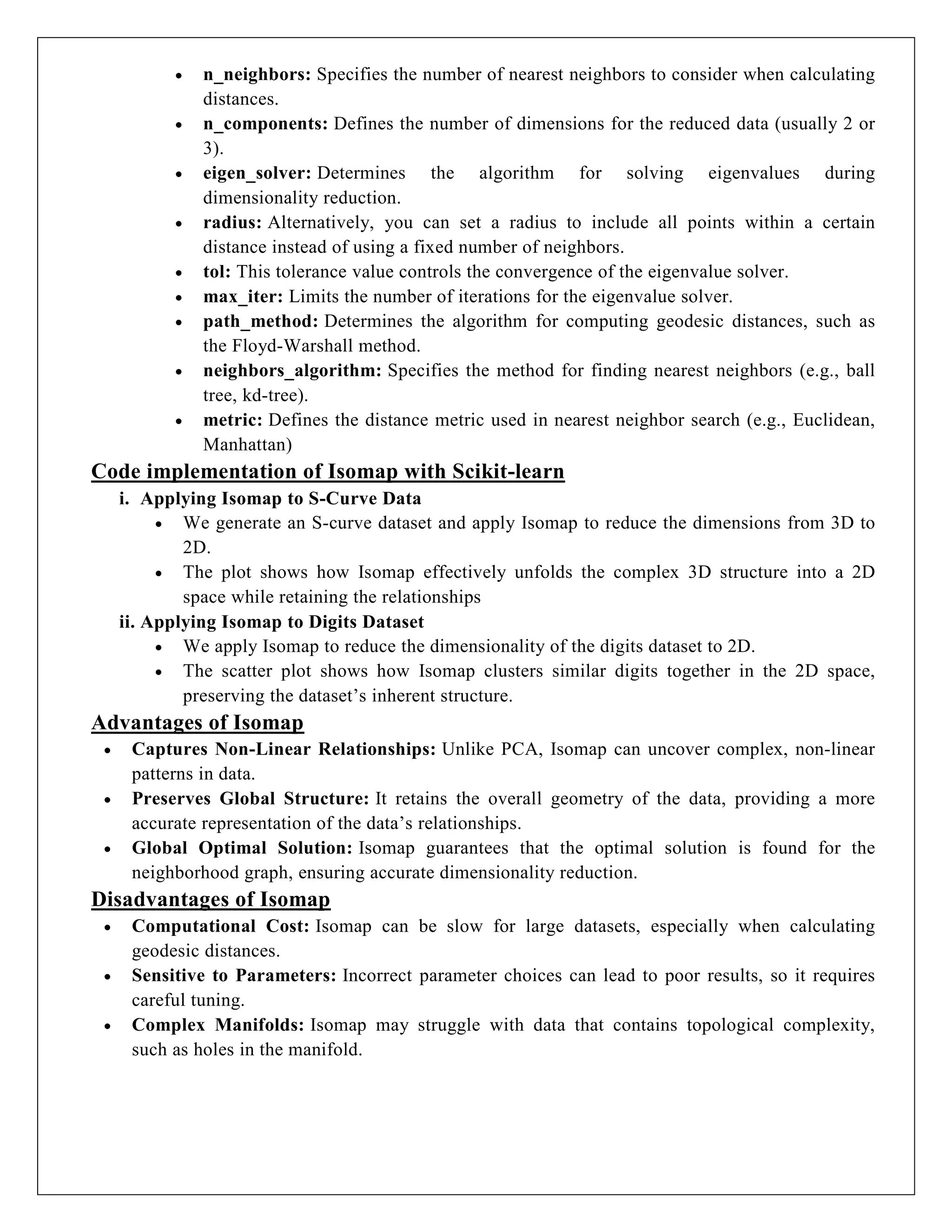
 n_neighbors: Specifies the number of nearest neighbors to consider when calculating
distances.
 n_components: Defines the number of dimensions for the reduced data (usually 2 or
3).
 eigen_solver: Determines the algorithm for solving eigenvalues during
dimensionality reduction.
 radius: Alternatively, you can set a radius to include all points within a certain
distance instead of using a fixed number of neighbors.
 tol: This tolerance value controls the convergence of the eigenvalue solver.
 max_iter: Limits the number of iterations for the eigenvalue solver.
 path_method: Determines the algorithm for computing geodesic distances, such as
the Floyd-Warshall method.
 neighbors_algorithm: Specifies the method for finding nearest neighbors (e.g., ball
tree, kd-tree).
 metric: Defines the distance metric used in nearest neighbor search (e.g., Euclidean,
Manhattan)
Code implementation of Isomap with Scikit-learn
i. Applying Isomap to S-Curve Data
 We generate an S-curve dataset and apply Isomap to reduce the dimensions from 3D to
2D.
 The plot shows how Isomap effectively unfolds the complex 3D structure into a 2D
space while retaining the relationships
ii. Applying Isomap to Digits Dataset
 We apply Isomap to reduce the dimensionality of the digits dataset to 2D.
 The scatter plot shows how Isomap clusters similar digits together in the 2D space,
preserving the dataset’s inherent structure.
Advantages of Isomap
 Captures Non-Linear Relationships: Unlike PCA, Isomap can uncover complex, non-linear
patterns in data.
 Preserves Global Structure: It retains the overall geometry of the data, providing a more
accurate representation of the data’s relationships.
 Global Optimal Solution: Isomap guarantees that the optimal solution is found for the
neighborhood graph, ensuring accurate dimensionality reduction.
Disadvantages of Isomap
 Computational Cost: Isomap can be slow for large datasets, especially when calculating
geodesic distances.
 Sensitive to Parameters: Incorrect parameter choices can lead to poor results, so it requires
careful tuning.
 Complex Manifolds: Isomap may struggle with data that contains topological complexity,
such as holes in the manifold.

Applications of Isomap
 Visualization: High-dimensional data, like face images, can be visualized in 2D or 3D,
making it easier to understand.
 Data Exploration: Isomap helps identify clusters and relationships that may not be obvious in
the original high-dimensional space.
 Anomaly Detection: Outliers or anomalies in the data can be identified by examining how
they deviate from the manifold.
 Pre-processing for Machine Learning: Isomap can be used as a pre-processing step before
applying other machine learning techniques, improving model performance.
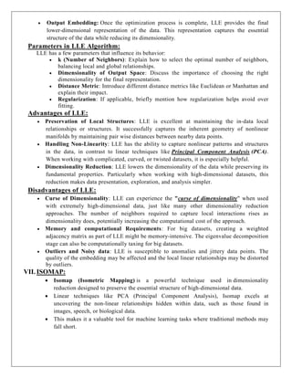
VIII. LEAST SQUARES OPTIMIZATION EVOLUTIONARY LEARNING:
 The Least Square method is a popular mathematical approach used in data fitting,
regression analysis, and predictive modeling.
 It helps find the best-fit line or curve that minimizes the sum of squared differences between
the observed data points and the predicted values.
 This technique is widely used in statistics, machine learning, and engineering applications.
Fig: Least Square Method
 Least Squares Method is used to derive a generalized linear equation between two variables.
 When the value of the dependent and independent variables they are represented as x and y
coordinates in a 2D Cartesian coordinate system.
 Initially, known values are marked on a plot. The plot obtained at this point is called a scatter
plot.
 Then, represent all the marked points as a straight line or a linear equation.
 The equation of such a line is obtained with the help of the Least Square method.
 This is done to get the value of the dependent variable for an independent variable for which
the value was initially unknown.
 This helps us to make predictions for the value of a dependent variable.

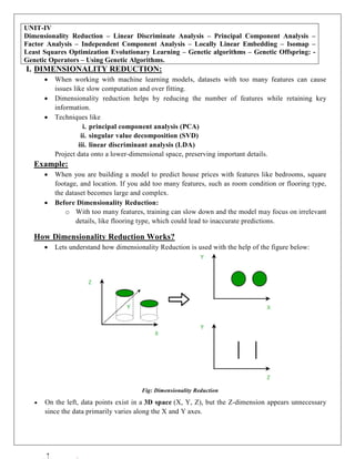
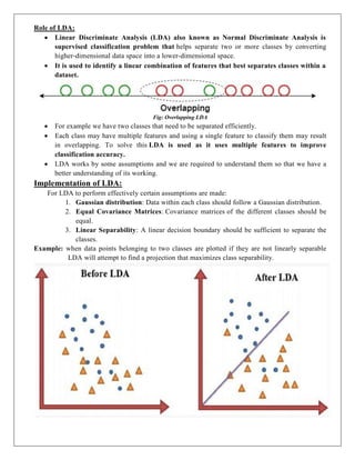
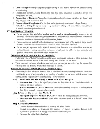
Why use the Least Square Method?
 In statistics, when the data can be represented on a Cartesian plane by using the independent
and dependent variables as the x and y coordinates, it is called scatter data.
 This data might not be useful in making interpretations or predicting the values of the
dependent variable for the independent variable.
 So, we try to get an equation of a line that fits best to the given data points with the help of
the Least Square Method.
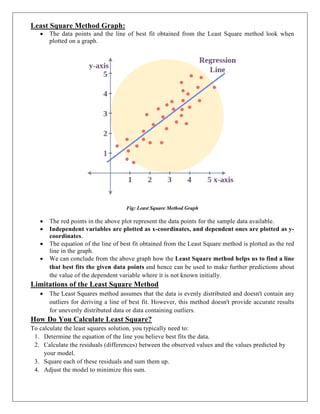
Least Square Method Formula
 The Least Square Method formula finds the best-fitting line through a set of data points.
 For a simple linear regression, which is a line of the form
y=mx+c
Where
y is the dependent variable,
x is the independent variable,
a is the slope of the line, and
b is the y-intercept,
The formulas to calculate the slope (m) and intercept (c) of the line are derived from the
following equations:
Where:
 n is the number of data points,
 ∑xy is the sum of the product of each pair of x and y values,
 ∑x is the sum of all x values,
 ∑y is the sum of all y values,
 ∑x2 is the sum of the squares of the x values.
Steps to find the line of Best Fit by using the Least Squares Method:
 Step 1: Denote the independent variable values as xi and the dependent ones as yi.
 Step 2: Calculate the average values of xi and yi as X and Y.
 Step 3: Presume the equation of the line of best fit as y = mx + c, where m is the slope of the
line and c represents the intercept of the line on the Y-axis.
 Step 4: The slope m can be calculated from the following formula:
m = [Σ (X - xi) × (Y - yi)] / Σ(X - xi)2
 Step 5: The intercept c is calculated from the following formula:
c = Y - mX
Thus, we obtain the line of best fit as y = mx + c, where values of m and c can be calculated
from the formulae defined above.
 These formulas are used to calculate the parameters of the line that best fits the data according
to the criterion of the least squares, minimizing the sum of the squared differences between
the observed values and the values predicted by the linear model.

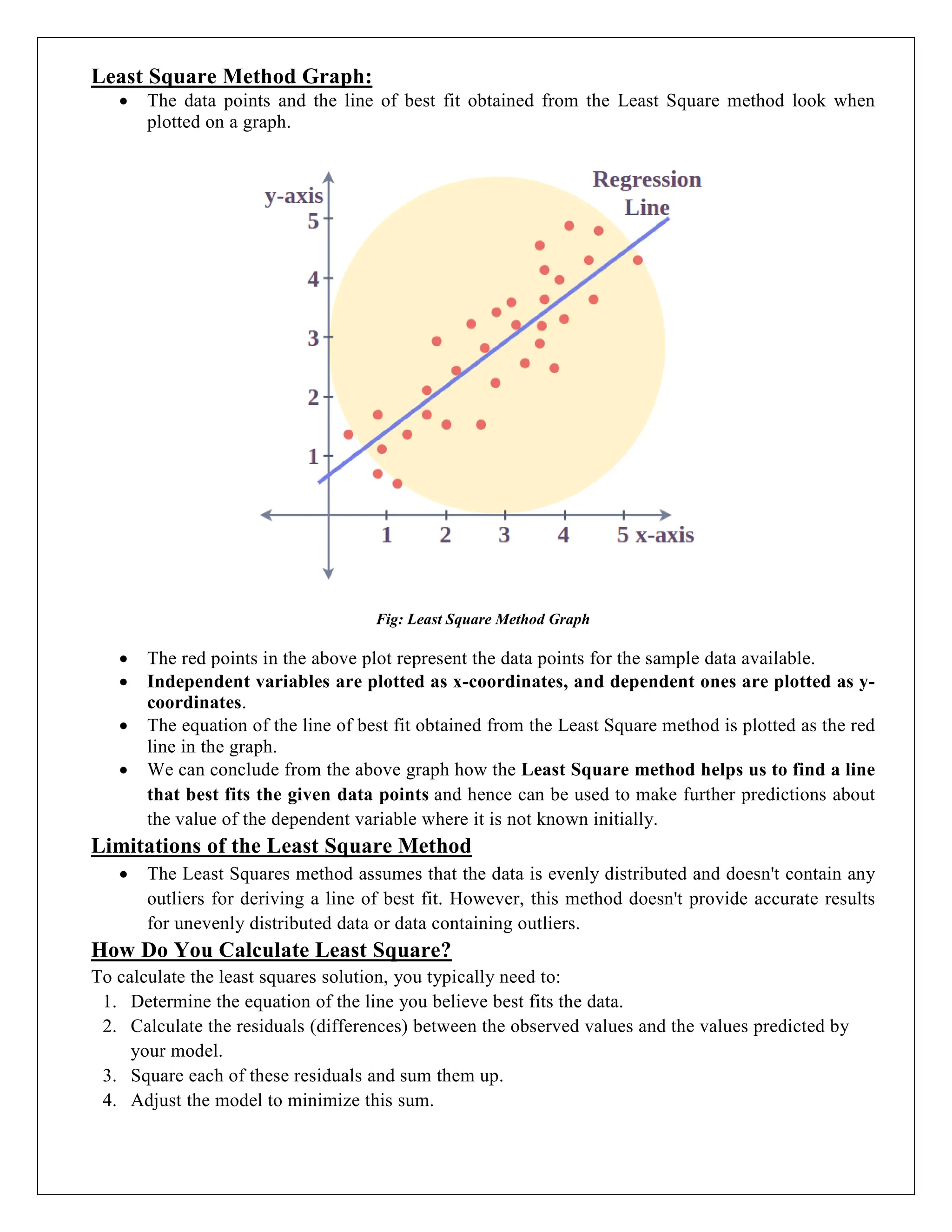
Least Square Method Graph:
 The data points and the line of best fit obtained from the Least Square method look when
plotted on a graph.
Fig: Least Square Method Graph
 The red points in the above plot represent the data points for the sample data available.
 Independent variables are plotted as x-coordinates, and dependent ones are plotted as y-
coordinates.
 The equation of the line of best fit obtained from the Least Square method is plotted as the red
line in the graph.
 We can conclude from the above graph how the Least Square method helps us to find a line
that best fits the given data points and hence can be used to make further predictions about
the value of the dependent variable where it is not known initially.
Limitations of the Least Square Method
 The Least Squares method assumes that the data is evenly distributed and doesn't contain any
outliers for deriving a line of best fit. However, this method doesn't provide accurate results
for unevenly distributed data or data containing outliers.
How Do You Calculate Least Square?
To calculate the least squares solution, you typically need to:
1. Determine the equation of the line you believe best fits the data.
2. Calculate the residuals (differences) between the observed values and the values predicted by
your model.
3. Square each of these residuals and sum them up.
4. Adjust the model to minimize this sum.

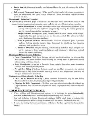
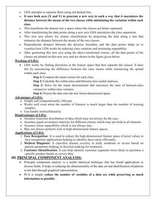
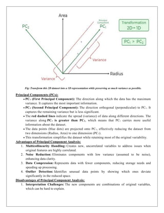
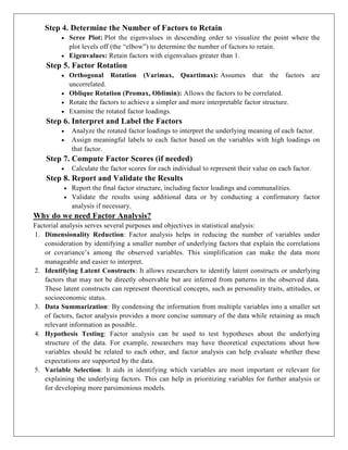
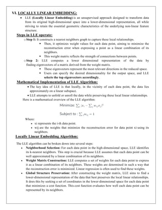
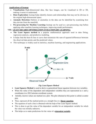
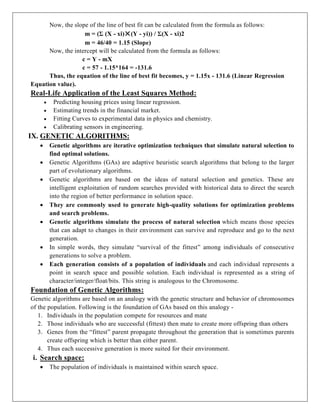
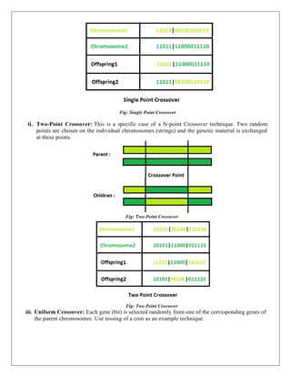
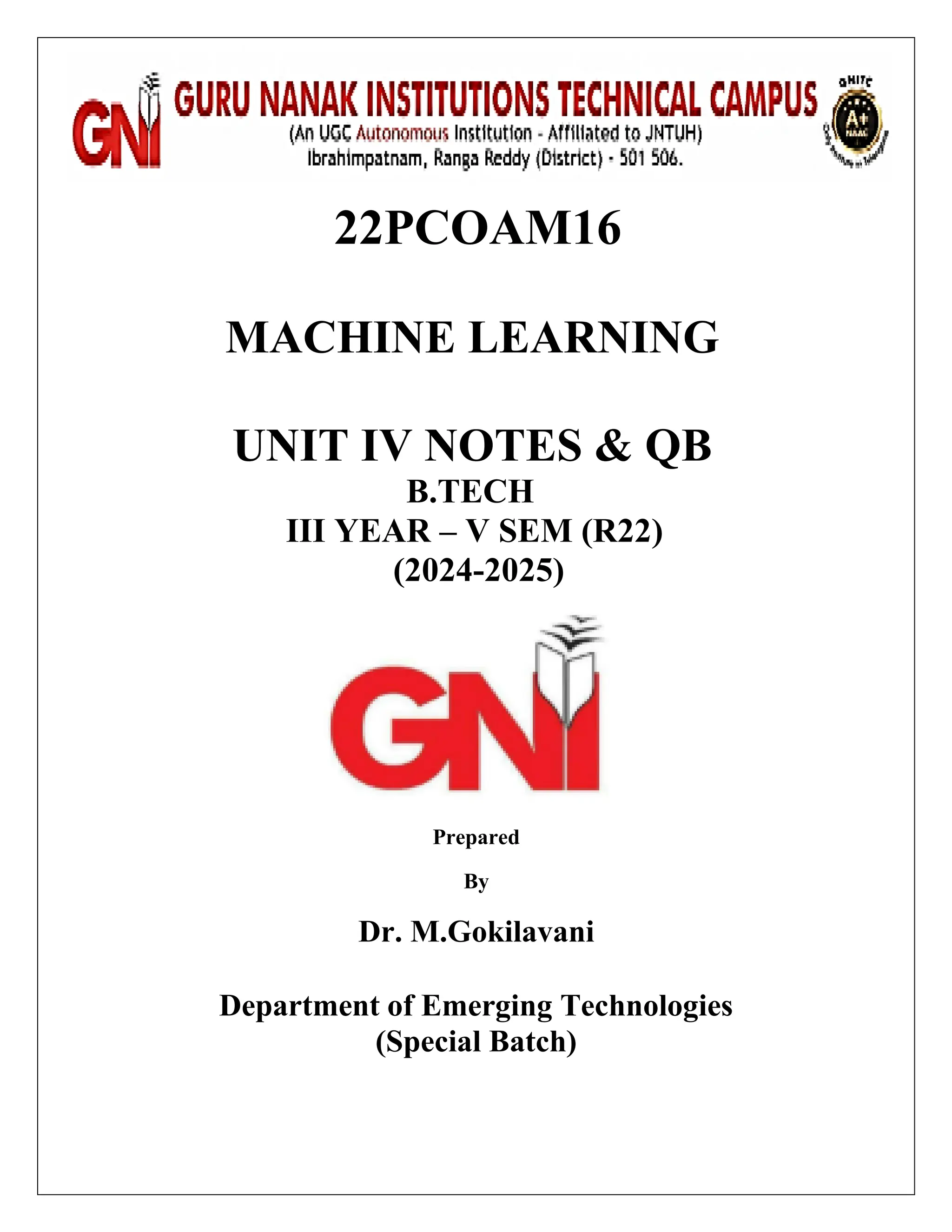
Least Square Method Solved Examples:
Problem 1: Find the line of best fit for the following data points using the Least Square method:
(x,y) = (1,3), (2,4), (4,8), (6,10), (8,15).
Solution:
Here, we have x as the independent variable and y as the dependent variable. First, we
calculate the means of x and y values denoted by X and Y respectively.
X = (1+2+4+6+8)/5 = 4.2
Y = (3+4+8+10+15)/5 = 8
xi yi X - xi Y - yi (X-xi)*(Y-yi) (X - xi)2
1 3 3.2 5 16 10.24
2 4 2.2 4 8.8 4.84
4 8 0.2 0 0 0.04
6 10 -1.8 -2 3.6 3.24
8 15 -3.8 -7 26.6 14.44
1 3 3.2 5 16 10.24
Sum (Σ) 0 0 55 32.8
The slope of the line of best fit can be calculated from the formula as follows:
m = (Σ (X - xi)*(Y - yi)) /Σ(X - xi)2
m = 55/32.8 = 1.68 (rounded upto 2 decimal places)
Now, the intercept will be calculated from the formula as follows:
c = Y - mX
c = 8 - 1.68*4.2 = 0.94
Thus, the equation of the line of best fit becomes, y = 1.68x + 0.94.
Problem 2: Find the line of best fit for the following data of heights and weights of students of a
school using the Least Squares method:
 Height (in centimeters): [160, 162, 164, 166, 168]
 Weight (in kilograms): [52, 55, 57, 60, 61]
Solution:
Here, we denote Height as x (independent variable) and Weight as y (dependent variable).
Now, we calculate the means of x and y values denoted by X and Y respectively.
X (Height) = (160 + 162 + 164 + 166 + 168) / 5 = 164
Y (Weight) = (52 + 55 + 57 + 60 + 61) / 5 = 57
xi yi X - xi Y - yi (X-xi)*(Y-yi) (X - xi)2
160 52 4 5 20 16
162 55 2 2 4 4
164 57 0 0 0 0
166 60 -2 -3 6 4
168 61 -4 -4 16 16
160 52 4 5 20 16
Sum (Σ) 0 0 55 32.8

Now, the slope of the line of best fit can be calculated from the formula as follows:
m = (Σ (X - xi)✕(Y - yi)) / Σ(X - xi)2
m = 46/40 = 1.15 (Slope)
Now, the intercept will be calculated from the formula as follows:
c = Y - mX
c = 57 - 1.15*164 = -131.6
Thus, the equation of the line of best fit becomes, y = 1.15x - 131.6 (Linear Regression
Equation value).
Real-Life Application of the Least Squares Method:
 Predicting housing prices using linear regression.
 Estimating trends in the financial market.
 Fitting Curves to experimental data in physics and chemistry.
 Calibrating sensors in engineering.
IX. GENETIC ALGORITHMS:
 Genetic algorithms are iterative optimization techniques that simulate natural selection to
find optimal solutions.
 Genetic Algorithms (GAs) are adaptive heuristic search algorithms that belong to the larger
part of evolutionary algorithms.
 Genetic algorithms are based on the ideas of natural selection and genetics. These are
intelligent exploitation of random searches provided with historical data to direct the search
into the region of better performance in solution space.
 They are commonly used to generate high-quality solutions for optimization problems
and search problems.
 Genetic algorithms simulate the process of natural selection which means those species
that can adapt to changes in their environment can survive and reproduce and go to the next
generation.
 In simple words, they simulate “survival of the fittest” among individuals of consecutive
generations to solve a problem.
 Each generation consists of a population of individuals and each individual represents a
point in search space and possible solution. Each individual is represented as a string of
character/integer/float/bits. This string is analogous to the Chromosome.
Foundation of Genetic Algorithms:
Genetic algorithms are based on an analogy with the genetic structure and behavior of chromosomes
of the population. Following is the foundation of GAs based on this analogy -
1. Individuals in the population compete for resources and mate
2. Those individuals who are successful (fittest) then mate to create more offspring than others
3. Genes from the “fittest” parent propagate throughout the generation that is sometimes parents
create offspring which is better than either parent.
4. Thus each successive generation is more suited for their environment.
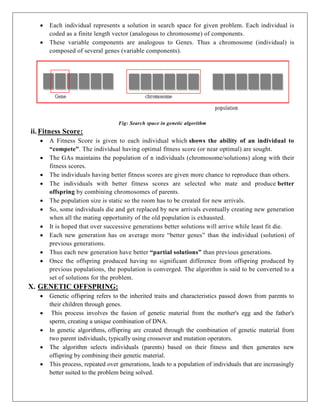
i. Search space:
 The population of individuals is maintained within search space.

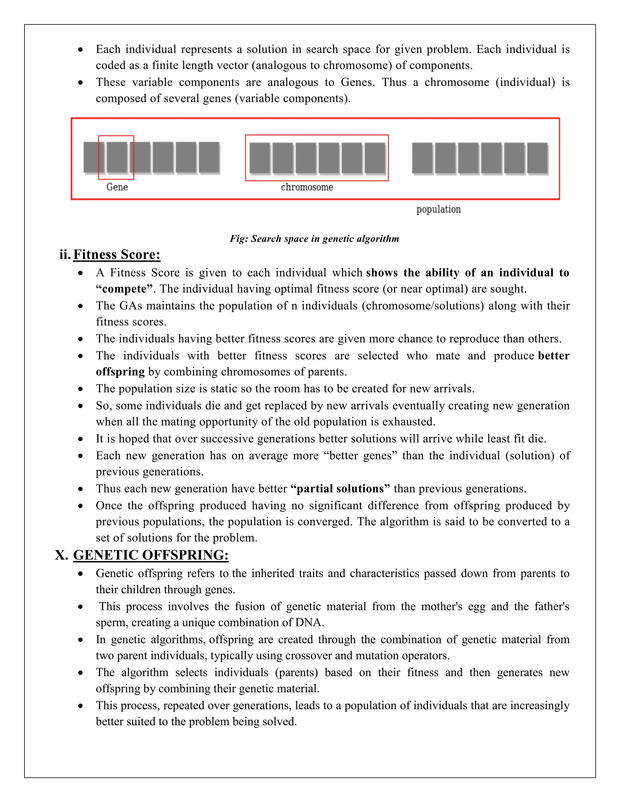
 Each individual represents a solution in search space for given problem. Each individual is
coded as a finite length vector (analogous to chromosome) of components.
 These variable components are analogous to Genes. Thus a chromosome (individual) is
composed of several genes (variable components).
Fig: Search space in genetic algorithm
ii.Fitness Score:
 A Fitness Score is given to each individual which shows the ability of an individual to
“compete”. The individual having optimal fitness score (or near optimal) are sought.
 The GAs maintains the population of n individuals (chromosome/solutions) along with their
fitness scores.
 The individuals having better fitness scores are given more chance to reproduce than others.
 The individuals with better fitness scores are selected who mate and produce better
offspring by combining chromosomes of parents.
 The population size is static so the room has to be created for new arrivals.
 So, some individuals die and get replaced by new arrivals eventually creating new generation
when all the mating opportunity of the old population is exhausted.
 It is hoped that over successive generations better solutions will arrive while least fit die.
 Each new generation has on average more “better genes” than the individual (solution) of
previous generations.
 Thus each new generation have better “partial solutions” than previous generations.
 Once the offspring produced having no significant difference from offspring produced by
previous populations, the population is converged. The algorithm is said to be converted to a
set of solutions for the problem.
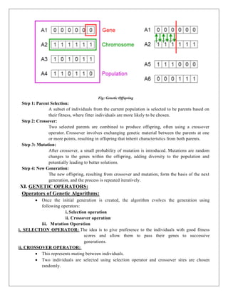
X. GENETIC OFFSPRING:
 Genetic offspring refers to the inherited traits and characteristics passed down from parents to
their children through genes.
 This process involves the fusion of genetic material from the mother's egg and the father's
sperm, creating a unique combination of DNA.
 In genetic algorithms, offspring are created through the combination of genetic material from
two parent individuals, typically using crossover and mutation operators.
 The algorithm selects individuals (parents) based on their fitness and then generates new
offspring by combining their genetic material.
 This process, repeated over generations, leads to a population of individuals that are increasingly
better suited to the problem being solved.

Fig: Genetic Offspring
Step 1: Parent Selection:
A subset of individuals from the current population is selected to be parents based on
their fitness, where fitter individuals are more likely to be chosen.
Step 2: Crossover:
Two selected parents are combined to produce offspring, often using a crossover
operator. Crossover involves exchanging genetic material between the parents at one
or more points, resulting in offspring that inherit characteristics from both parents.
Step 3: Mutation:
After crossover, a small probability of mutation is introduced. Mutations are random
changes to the genes within the offspring, adding diversity to the population and
potentially leading to better solutions.
Step 4: New Generation:
The new offspring, resulting from crossover and mutation, form the basis of the next
generation, and the process is repeated iteratively.
XI. GENETIC OPERATORS:
Operators of Genetic Algorithms:
 Once the initial generation is created, the algorithm evolves the generation using
following operators:
i. Selection operation
ii. Crossover operation
iii. Mutation Operation
i. SELECTION OPERATOR: The idea is to give preference to the individuals with good fitness
scores and allow them to pass their genes to successive
generations.
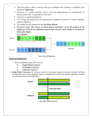
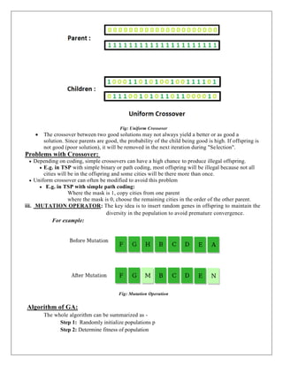
ii. CROSSOVER OPERATOR:
 This represents mating between individuals.
 Two individuals are selected using selection operator and crossover sites are chosen
randomly.

 Then the genes at these crossover sites are exchanged thus creating a completely new
individual (offspring).
 Crossover is a genetic operator used to vary the programming of a chromosome or
chromosomes from one generation to the next.
 Crossover is sexual reproduction.
 Two strings are picked from the mating pool at random to crossover in order to produce
superior offspring.
 The method chosen depends on the Encoding Method.
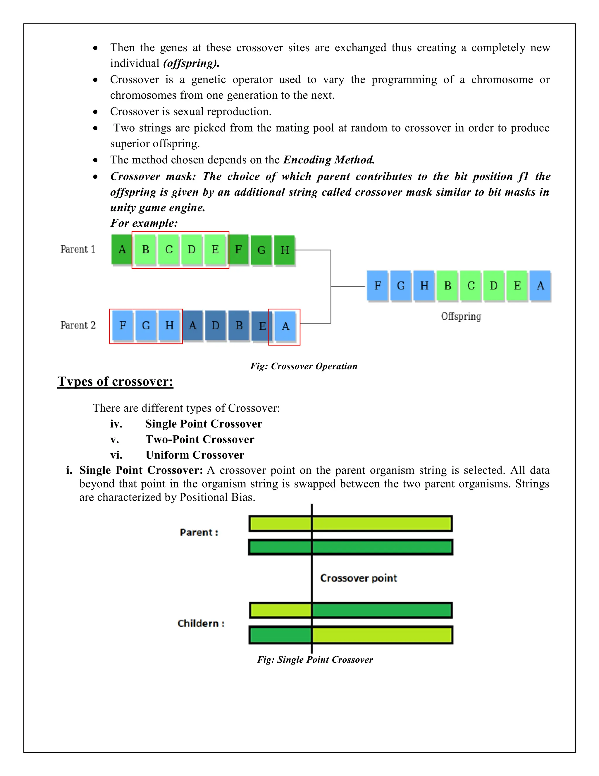
 Crossover mask: The choice of which parent contributes to the bit position f1 the
offspring is given by an additional string called crossover mask similar to bit masks in
unity game engine.
For example:
Fig: Crossover Operation
Types of crossover:
There are different types of Crossover:
iv. Single Point Crossover
v. Two-Point Crossover
vi. Uniform Crossover
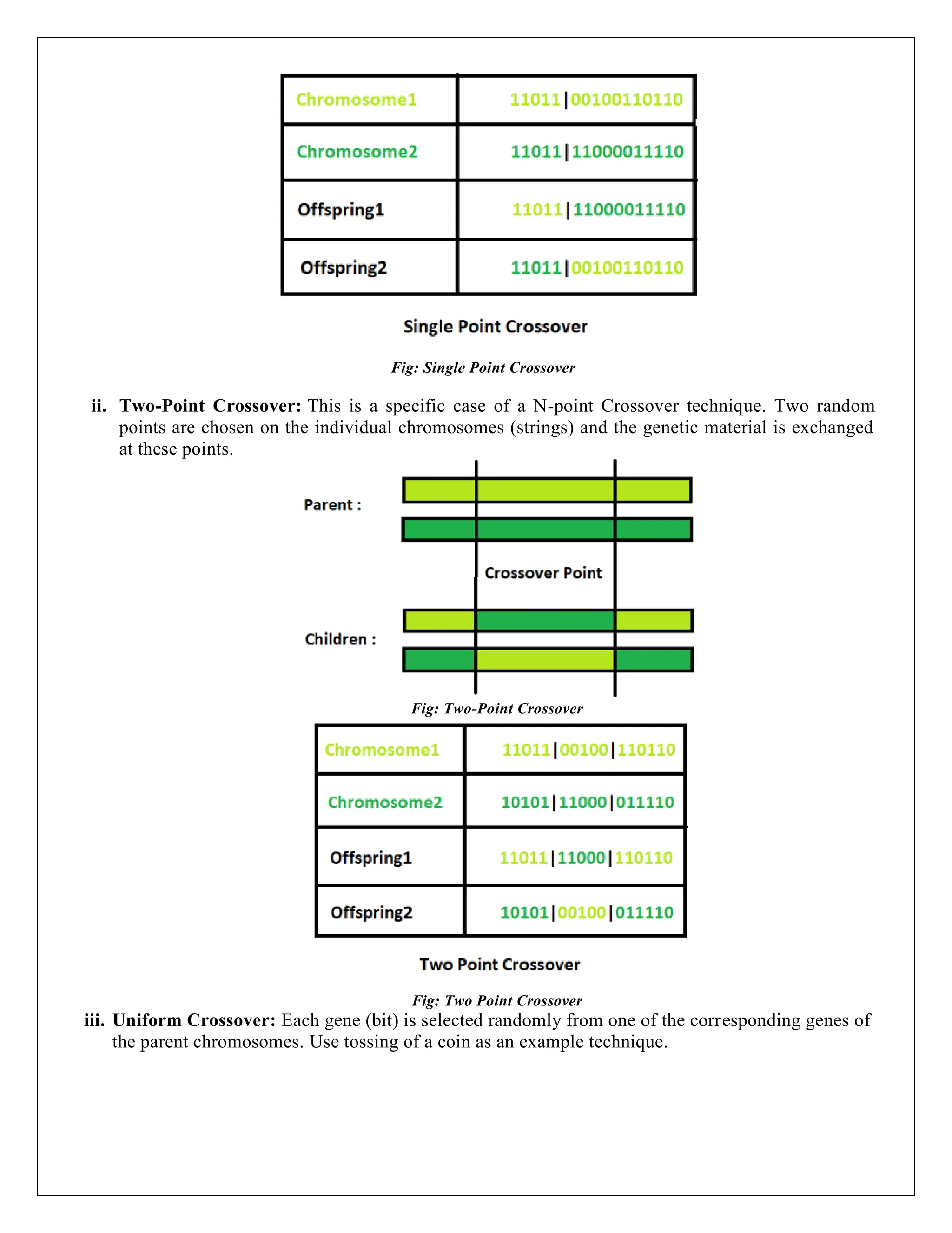
i. Single Point Crossover: A crossover point on the parent organism string is selected. All data
beyond that point in the organism string is swapped between the two parent organisms. Strings
are characterized by Positional Bias.
Fig: Single Point Crossover

Fig: Single Point Crossover
ii. Two-Point Crossover: This is a specific case of a N-point Crossover technique. Two random
points are chosen on the individual chromosomes (strings) and the genetic material is exchanged
at these points.
Fig: Two-Point Crossover
Fig: Two Point Crossover
iii. Uniform Crossover: Each gene (bit) is selected randomly from one of the corresponding genes of
the parent chromosomes. Use tossing of a coin as an example technique.

Fig: Uniform Crossover
 The crossover between two good solutions may not always yield a better or as good a
solution. Since parents are good, the probability of the child being good is high. If offspring is
not good (poor solution), it will be removed in the next iteration during "Selection".
Problems with Crossover:
 Depending on coding, simple crossovers can have a high chance to produce illegal offspring.
 E.g. in TSP with simple binary or path coding, most offspring will be illegal because not all
cities will be in the offspring and some cities will be there more than once.
 Uniform crossover can often be modified to avoid this problem
 E.g. in TSP with simple path coding:
Where the mask is 1, copy cities from one parent
where the mask is 0, choose the remaining cities in the order of the other parent.
iii. MUTATION OPERATOR: The key idea is to insert random genes in offspring to maintain the
diversity in the population to avoid premature convergence.
For example:
Fig: Mutation Operation
Algorithm of GA:
The whole algorithm can be summarized as -
Step 1: Randomly initialize populations p
Step 2: Determine fitness of population

Step 3: until convergence repeat:
Step 3.1: Select parents from population.
Step 3.2: Crossover and generate new population.
Step 3.3: Perform mutation on new population.
Step 3.4: Calculate fitness for new population.
XII. USING GENETIC ALGORITHMS
Example:
Given a target string, the goal is to produce target string starting from a random string of the same
length. In the following implementation, following analogies are made -
 Characters A-Z, a-z, 0-9, and other special symbols are considered as genes
 A string generated by these characters is considered as chromosome/solution/Individual.
STEPSIN GENETICALGORITHM:
 A genetic algorithm goes through a series of steps that mimic natural evolutionary processes
to find optimal solutions. These steps allow the population to evolve over generations,
improving the quality of solutions. Here is a general guideline for how a genetic algorithm
proceeds:
Step 1: Initialization
o First, we generate an initial population of random individuals. This step creates a diverse
set of potential solutions to start the algorithm.
Step 2: Evaluation
o Next, we need to calculate the fitness of each individual in the population. Here we use
the fitness function to evaluate how good each solution is.
Step 3: Selection
o Using the selection criteria, we select individuals for reproduction based on their fitness.
This step determines which individuals will be parents.
Step 4: Crossover
o Crossover comes next. By combining the genetic material of selected parents, we apply
crossover techniques to generate new solutions or offspring.
Step 5: Mutation
o To maintain diversity in our population, we need to introduce random mutations in the
offspring.
Step 6: Replacement
o We next replace some or all of the old population with the new offspring, by determining
which individuals move on to the next generation.
Step 7: Repeat
o The previous steps 2-6 are looped over for a set number of generations or until a
termination condition is met. This loop allows the population to evolve over time,
hopefully resulting in a good solution.
Examples of Genetic Offspring:
 Genetic inheritance describes how traits and characteristics are passed down from parents to their
offspring through genes.
 These genes, which are segments of DNA, carry instructions for various aspects of development
and function, including physical traits like eye color, hair color, and even predisposition to
certain health conditions.

Here are some examples of genetic inheritance in offspring:
 Eye color:
Different alleles (versions of a gene) determine whether someone will have blue,
brown, green, or hazel eyes.
 Blood type:
The ABO blood group system is an example of multiple alleles, with the different
types (A, B, AB, O) determined by combinations of inherited genes.
 Curly hair:
Some individuals inherit genes that cause their hair to grow in a curly or wavy
pattern.
 Handedness:
Whether someone is naturally right-handed or left-handed can be influenced by
genetic factors.
 Genetic disorders:
Certain diseases, such as cystic fibrosis, sickle cell disease, and hemophilia, can be
passed down through families if a parent carries a mutated gene.
 Height:
While height is influenced by many factors, including environment, genetics also
play a significant role, with some individuals inheriting genes that make them
predisposed to being taller or shorter.
Examples of Inheritance Patterns:
 Autosomal Dominant:
A single copy of a mutated gene is sufficient to cause a disease (e.g., Huntington's
disease, Marfan syndrome).
 Autosomal Recessive:
Two copies of a mutated gene are needed for a disease to manifest (e.g., cystic
fibrosis, sickle cell disease).
 X-linked Dominant:
The gene responsible is located on the X chromosome, and a single copy of the
mutated gene in females or males can cause the disease (e.g., fragile X
syndrome).
 X-linked Recessive:
The gene responsible is located on the X chromosome, and females need two
copies of the mutated gene while males only need one to develop the disease
(e.g., hemophilia).
Application of Genetic Algorithms:
Genetic algorithms have many applications, some of them are -
 Recurrent Neural Network
 Mutation testing
 Code breaking
 Filtering and signal processing
 Learning fuzzy rule base etc.

22PCOAM16_MACHINE_LEARNING_UNIT_IV_NOTES_with_QB

More Related Content

What's hot

Similar to 22PCOAM16_MACHINE_LEARNING_UNIT_IV_NOTES_with_QB

More from Guru Nanak Technical Institutions

Recently uploaded

22PCOAM16_MACHINE_LEARNING_UNIT_IV_NOTES_with_QB