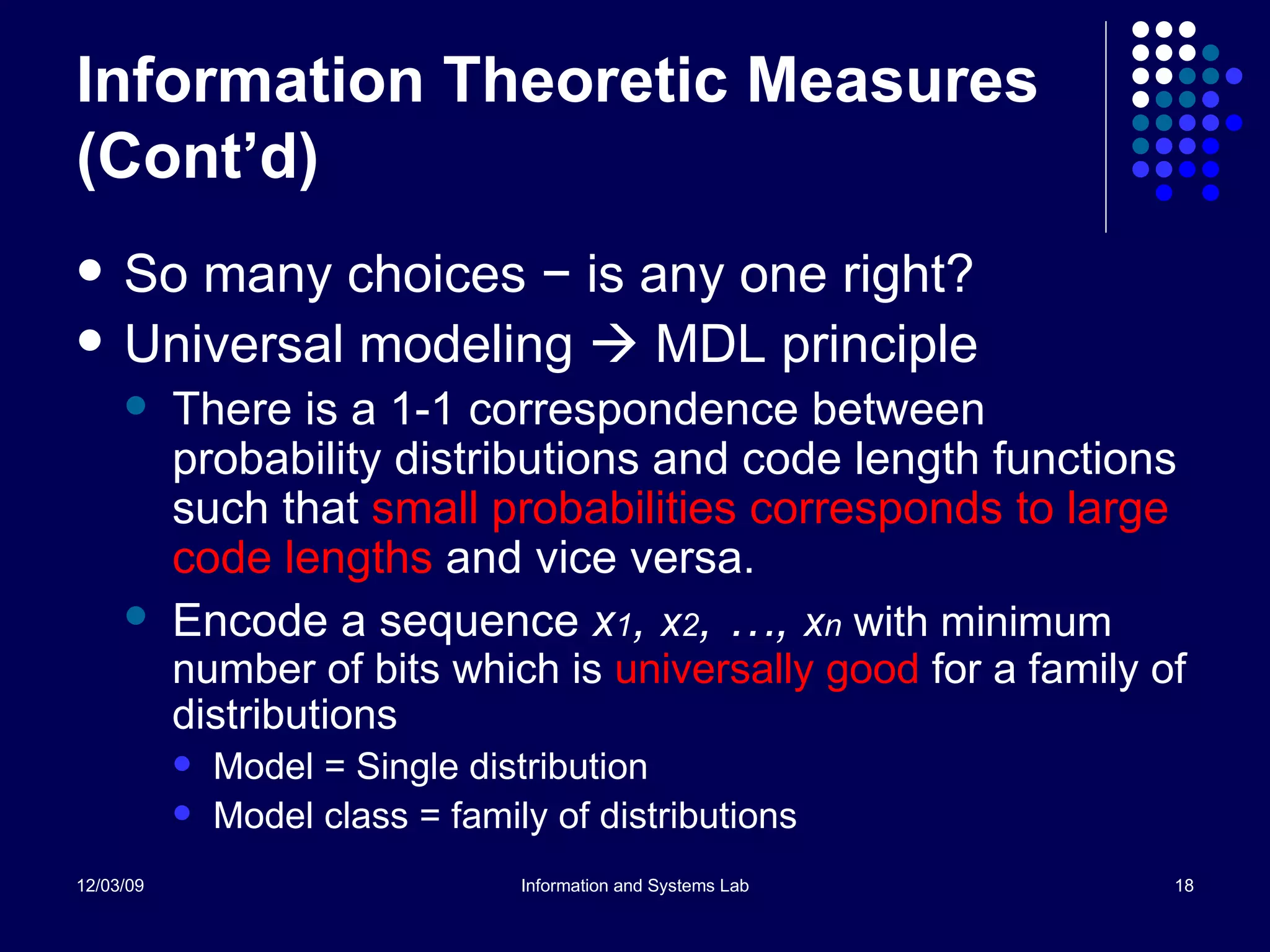
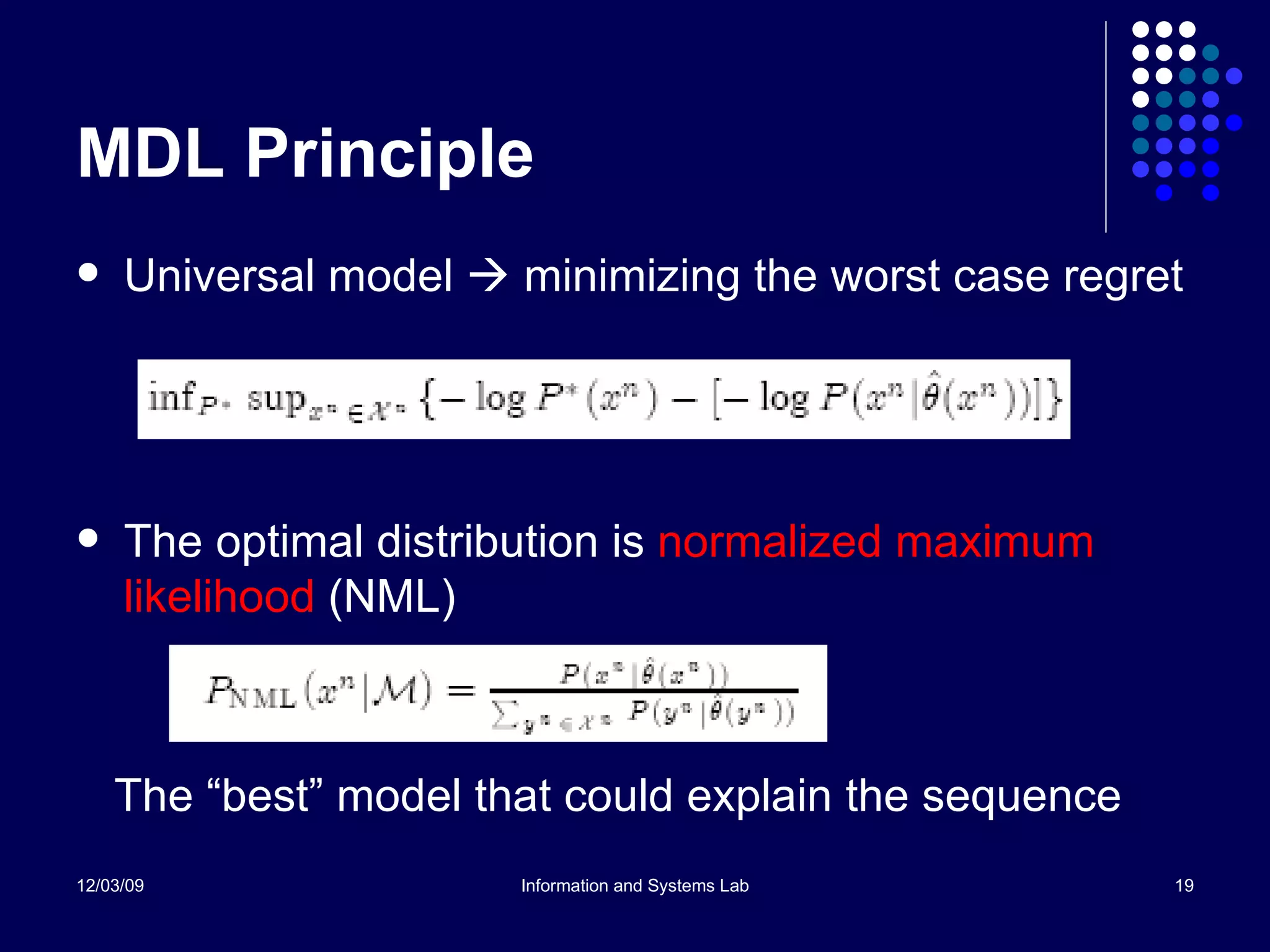
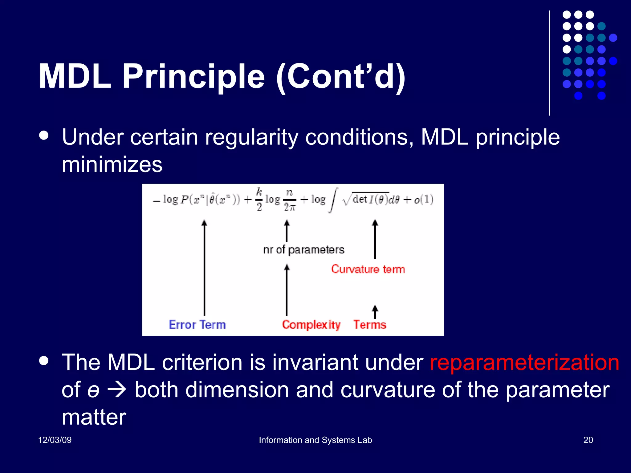
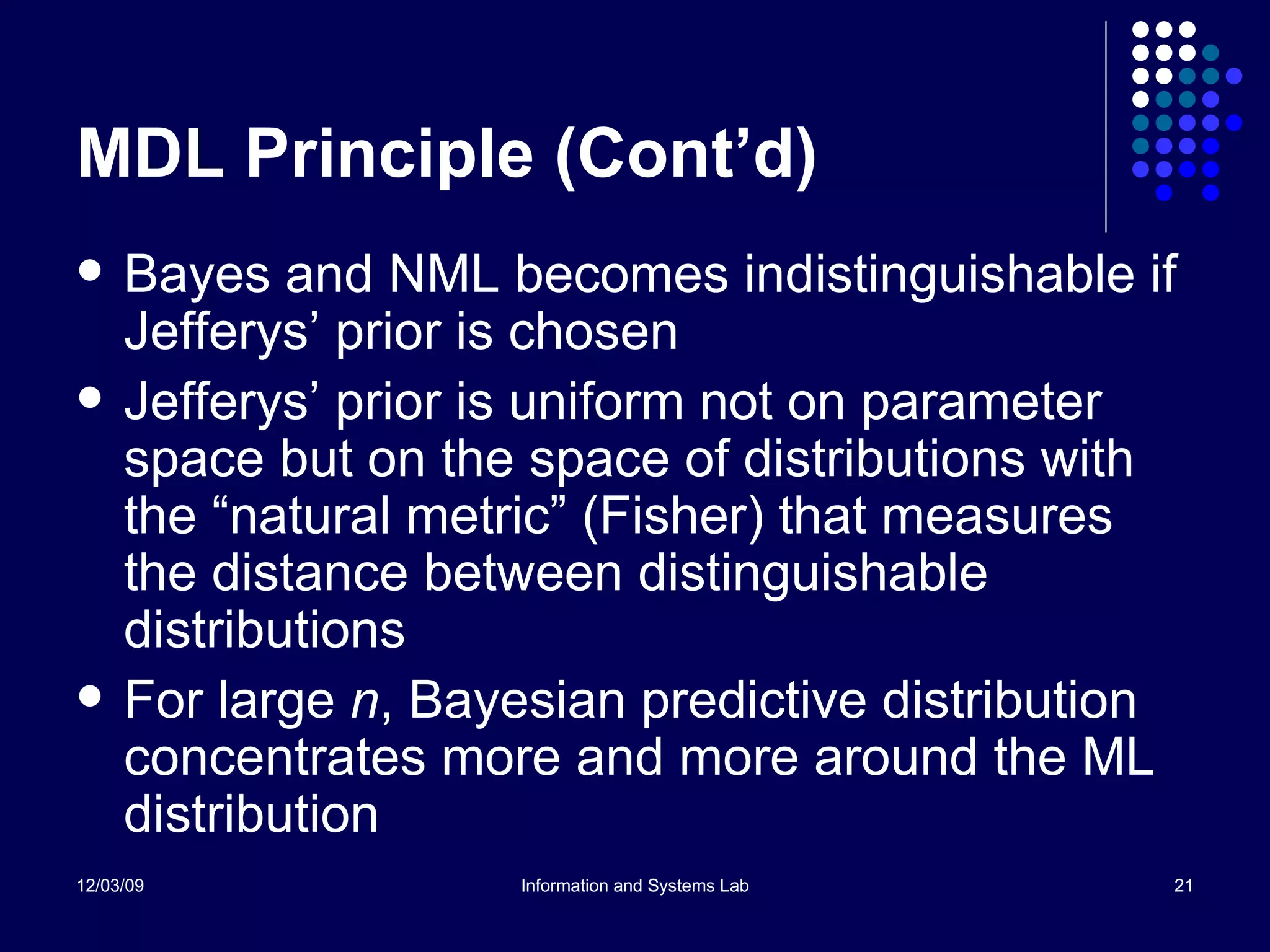
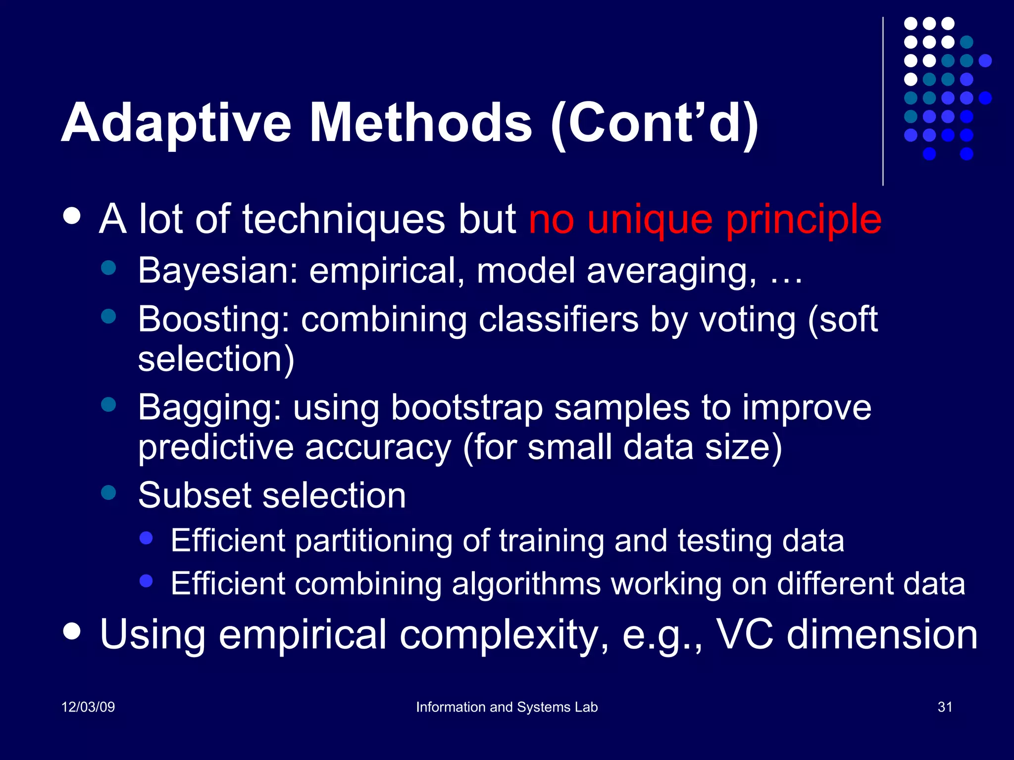
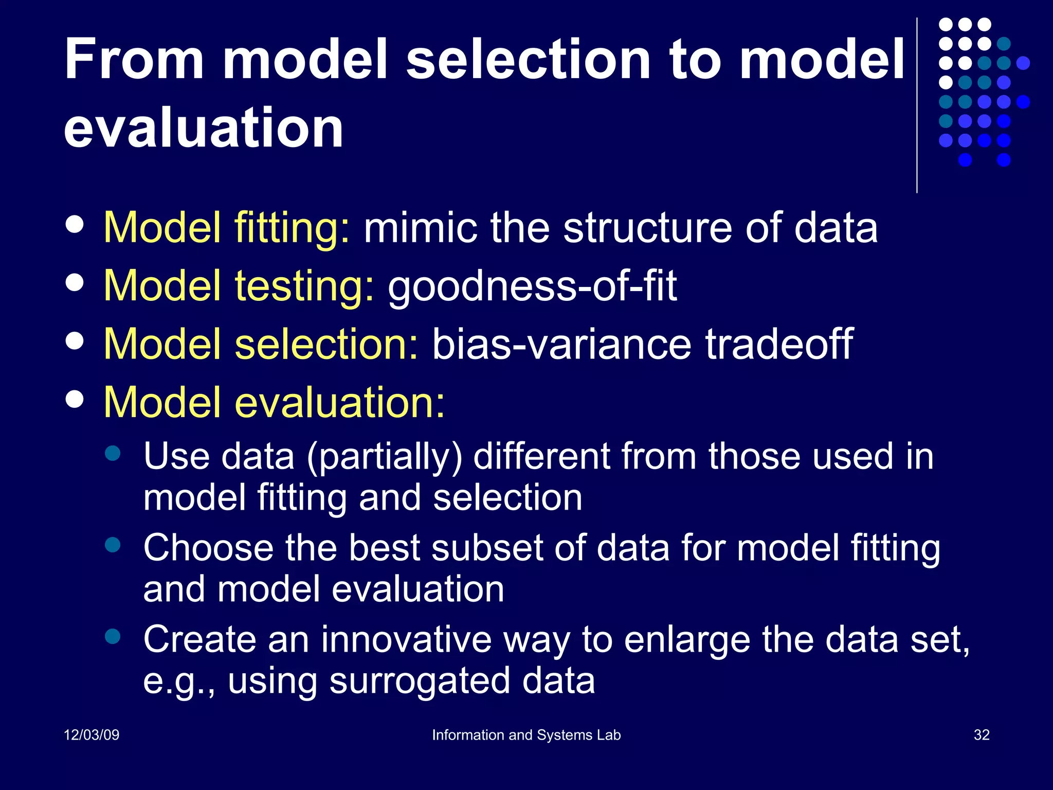
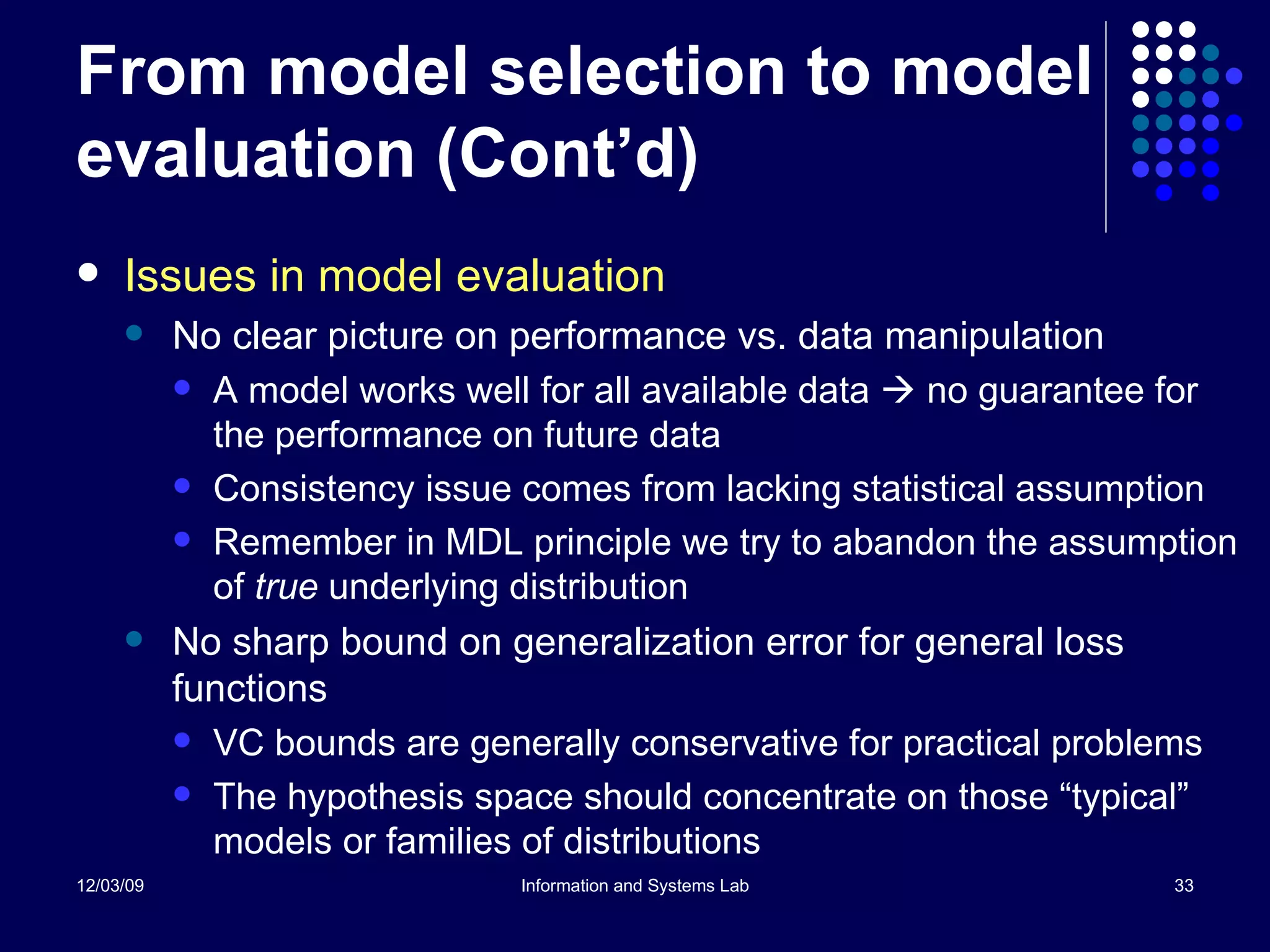
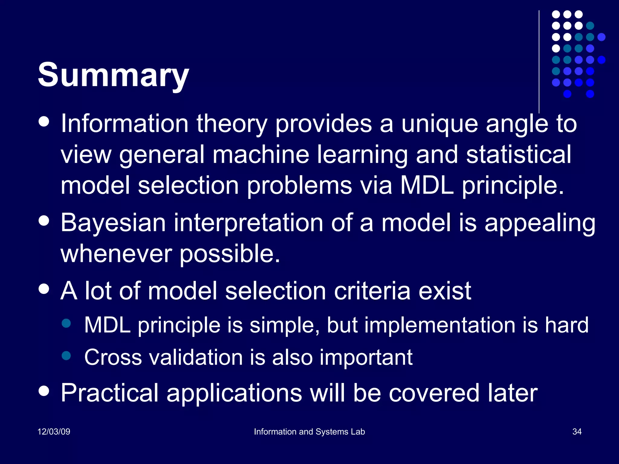
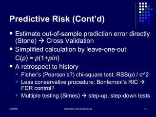
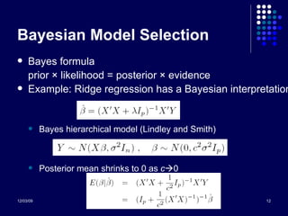
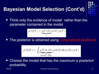
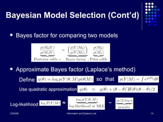
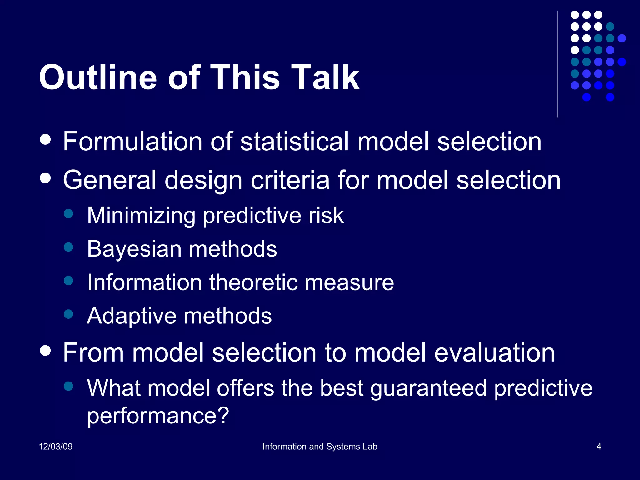
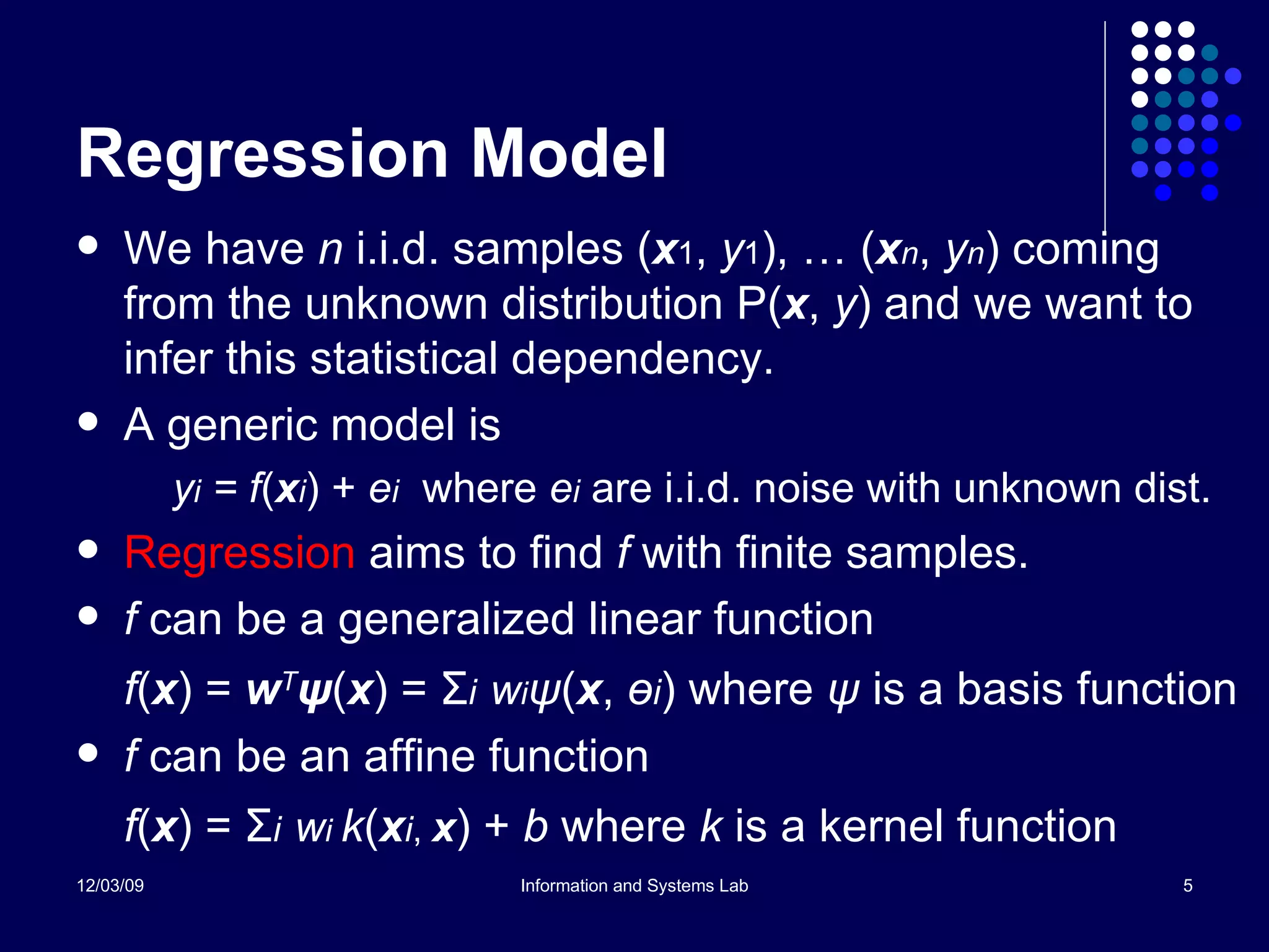
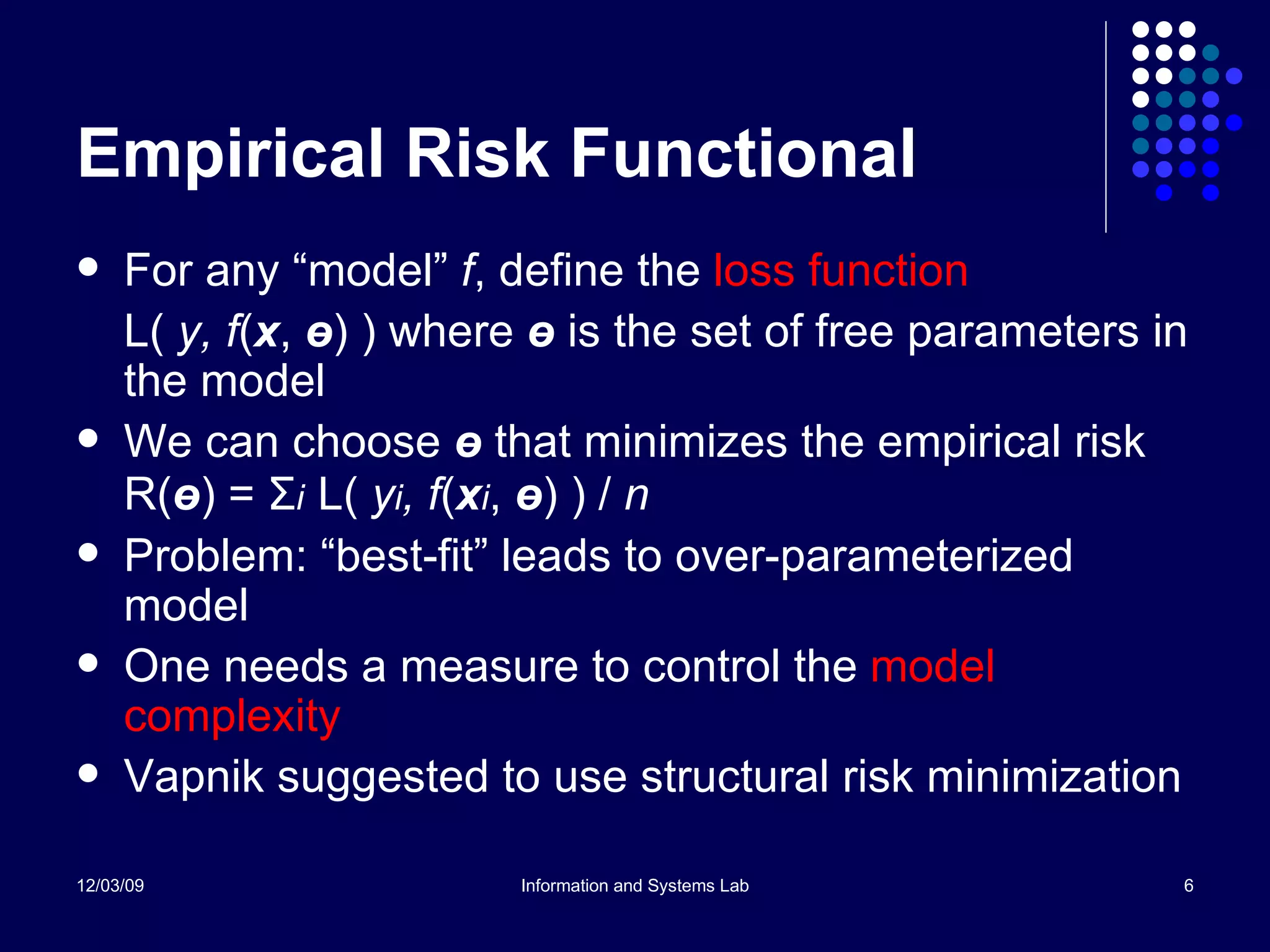
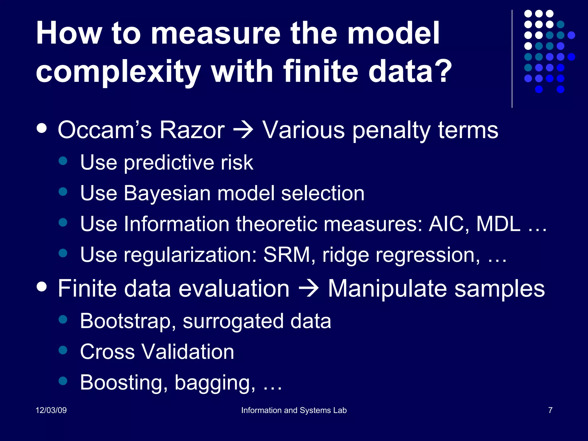
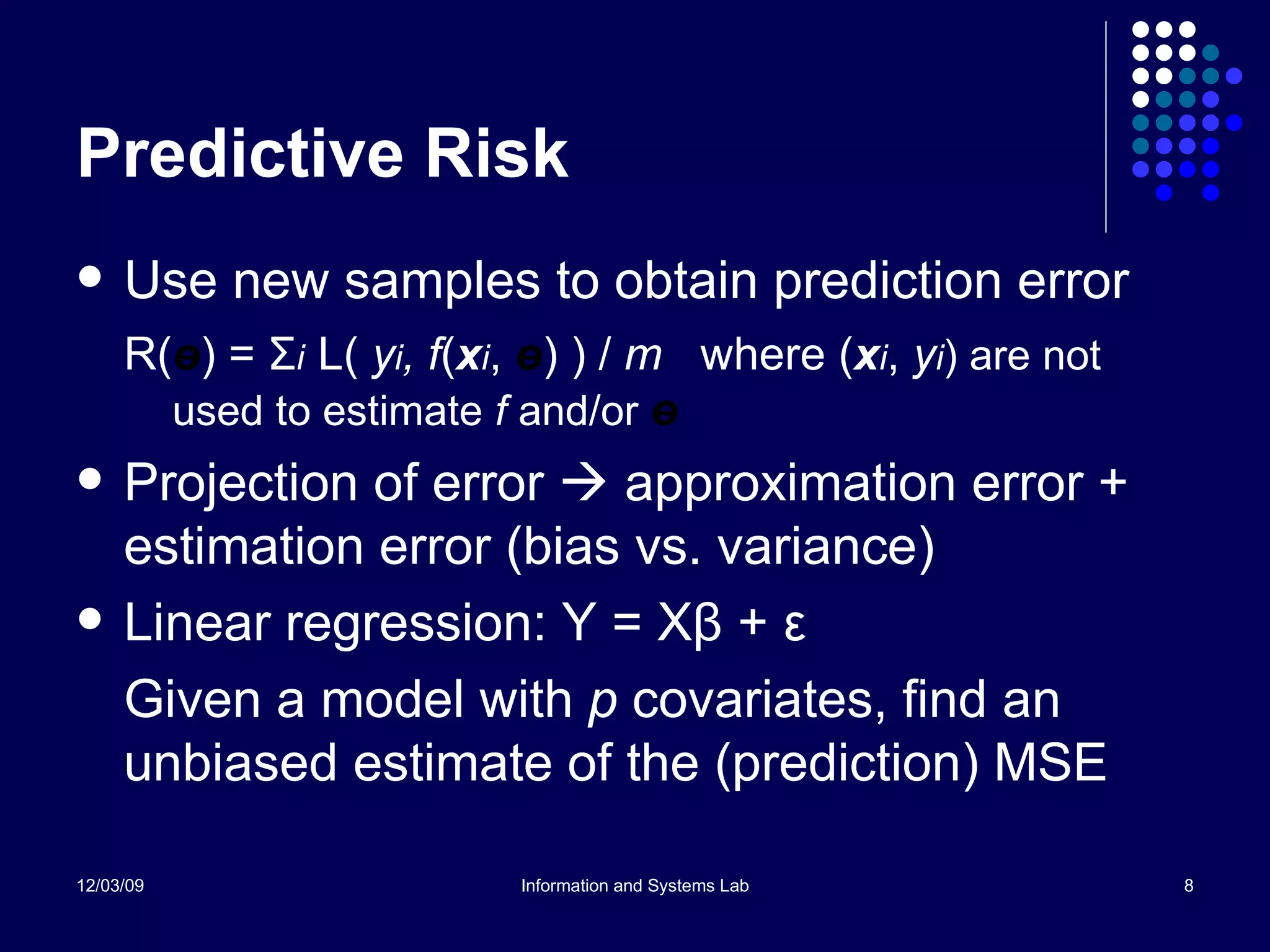
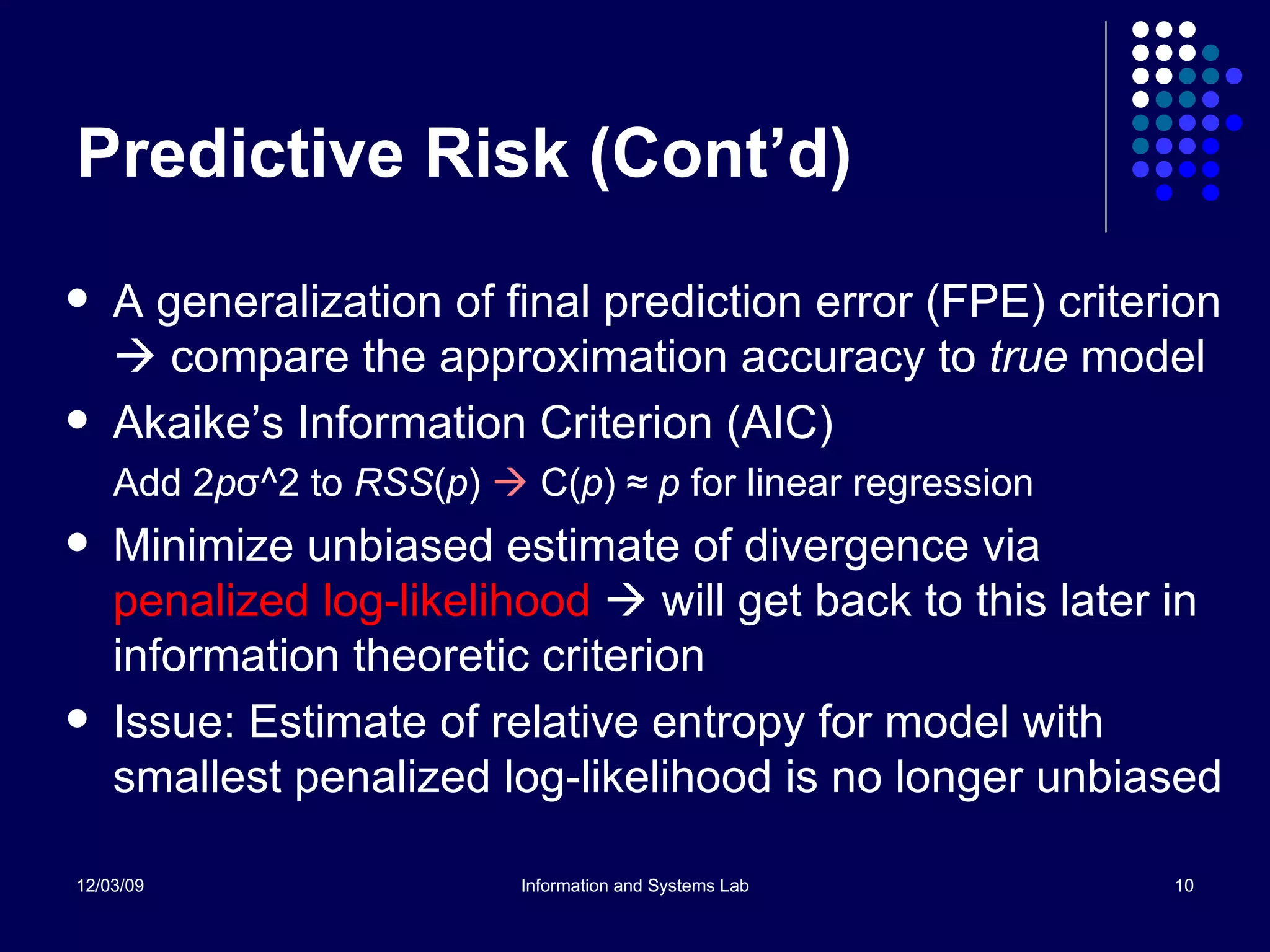
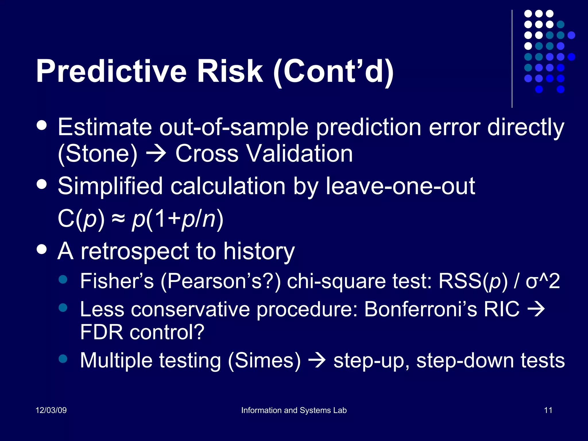
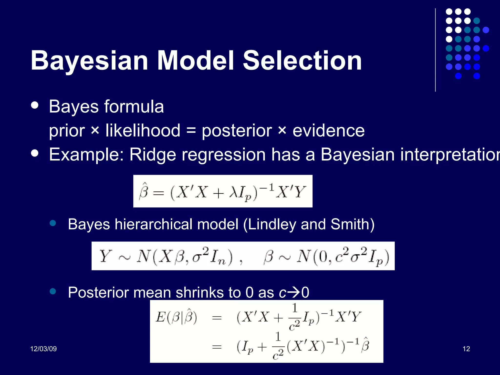
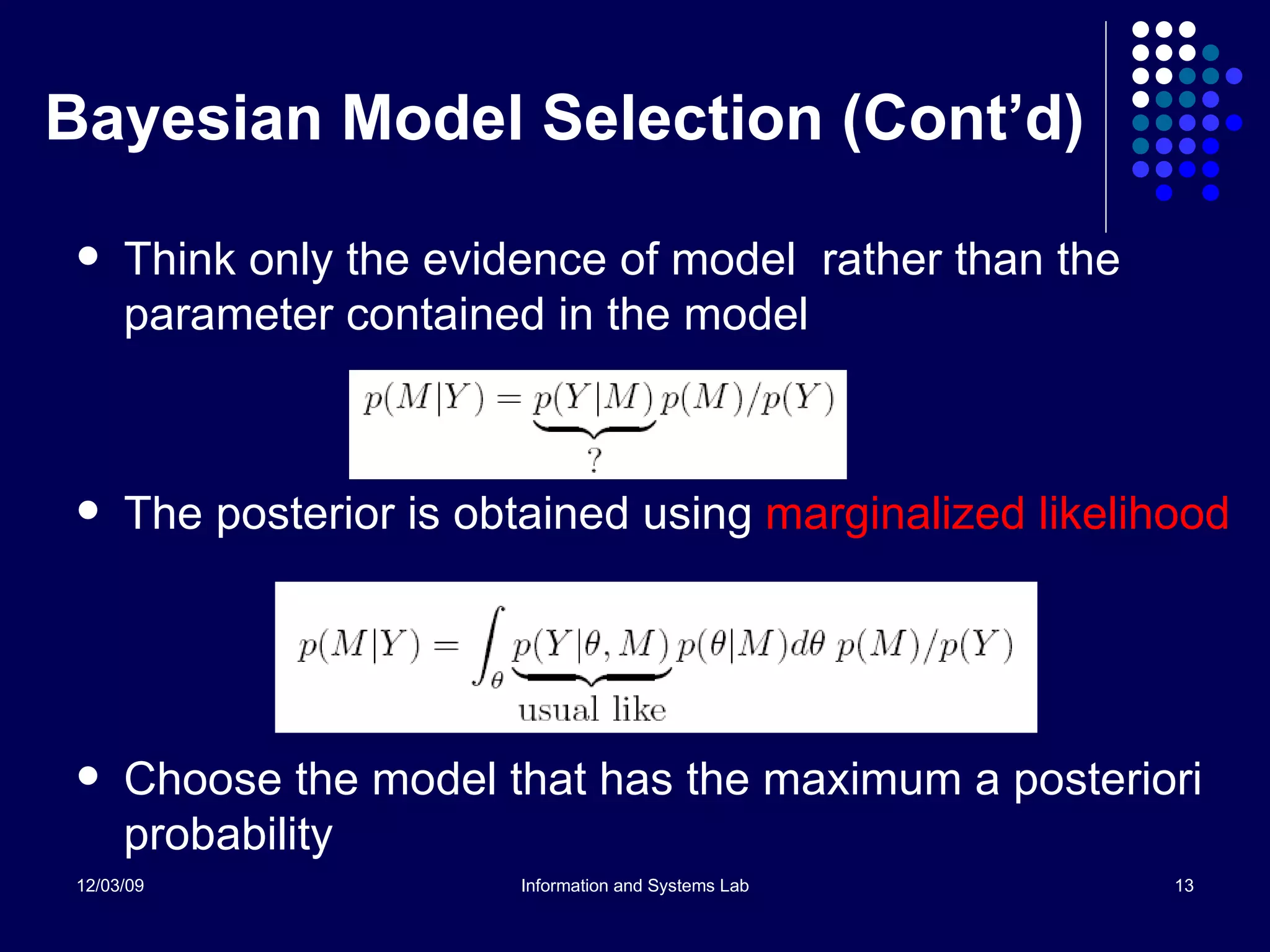
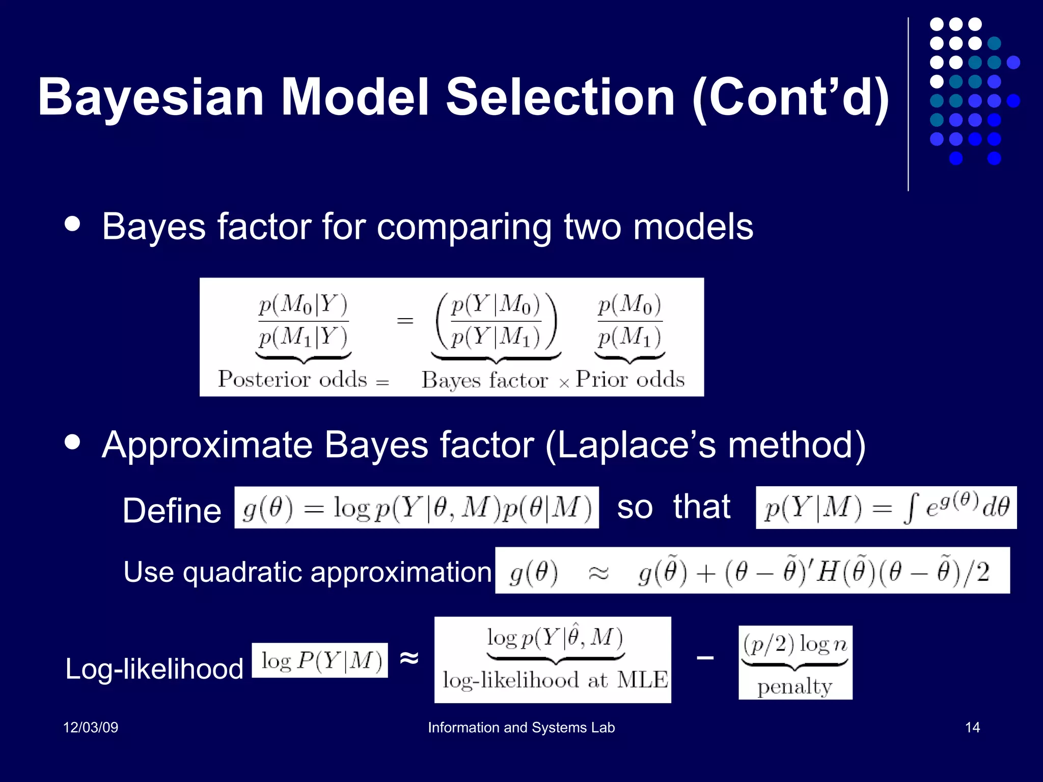
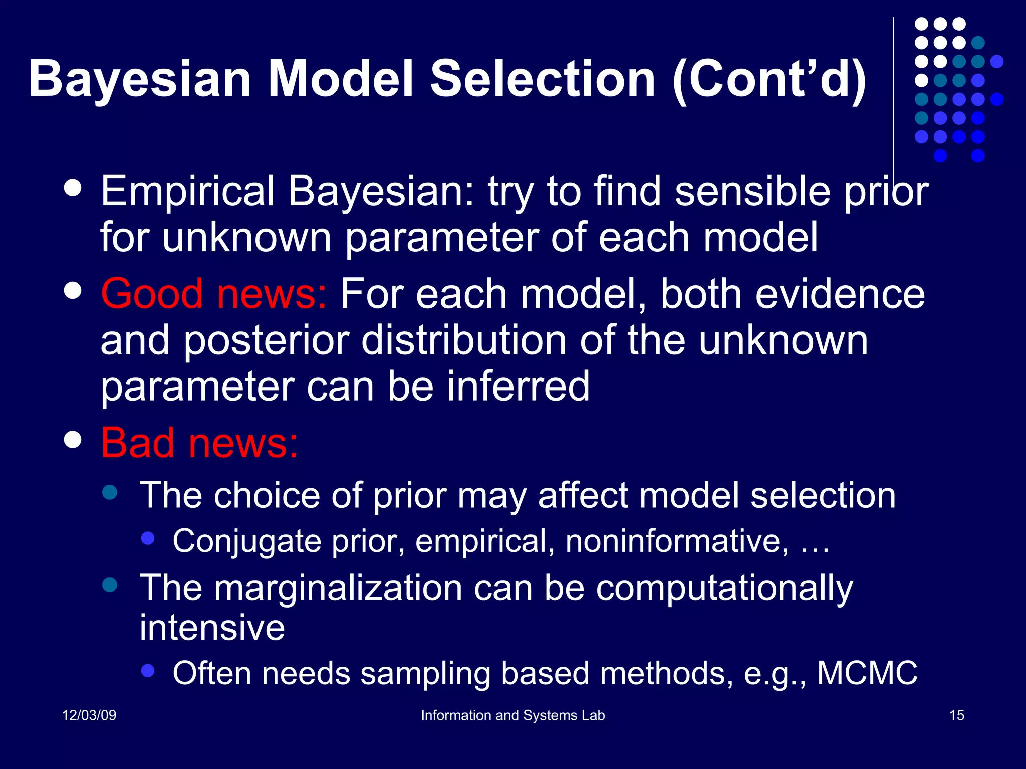
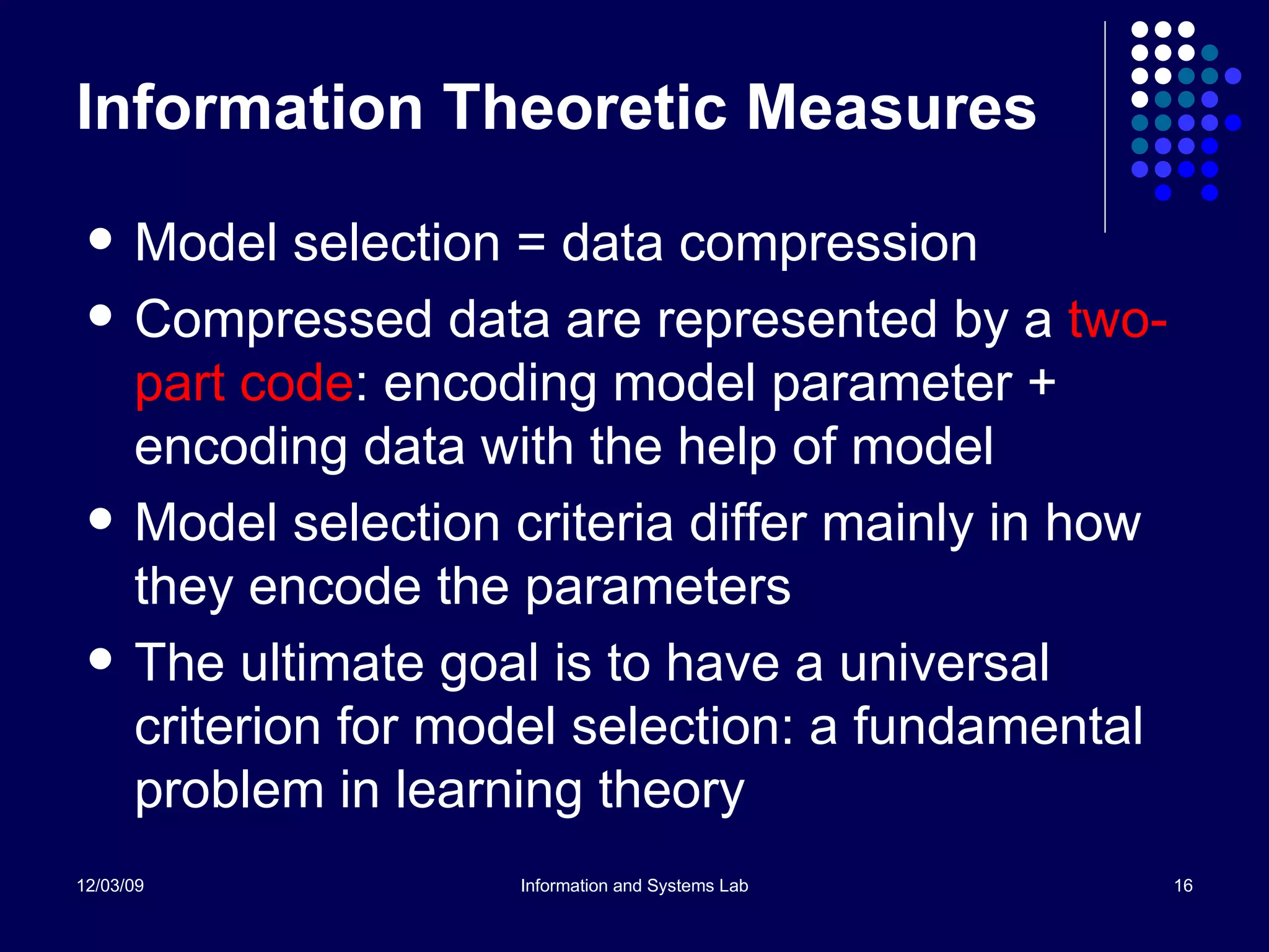
KEMBAR78
Intro to Model Selection | PPT
Introduction to Statistical Model Selection Huimin Chen Department of Electrical Engineering University of New Orleans New Orleans, LA 70148
Typical Problem Model: explaining available data, predicting new observations … But we do not know the real model Unsure about true data generation mechanism Unsure of which predictors are useful Model set can be huge or even with infinite elements Have to narrow down to  statistical models
Modeling and  Model Selection Variable selection Which factors are important What statistical dependencies are significant Most problems are  learning from data Bias-Variance Tradeoff Key is to understand/interpret  penalty  terms Goodness of fit vs. model complexity Other computational issues Dimension reduction, optimization …
Outline of This Talk Formulation of statistical model selection General design criteria for model selection Minimizing predictive risk Bayesian methods Information theoretic measure Adaptive methods From model selection to model evaluation What model offers the best guaranteed predictive performance?
Regression Model We have  n  i.i.d. samples ( x 1 ,  y 1 ), … ( x n ,  y n ) coming from the unknown distribution P( x ,  y ) and we want to infer this statistical dependency. A generic model is y i  = f ( x i ) +  e i   where  e i  are i.i.d. noise with unknown dist. Regression  aims to find  f  with finite samples. f  can be a generalized linear function f ( x ) =  w T ψ ( x ) =  Σ i   w i ψ ( x ,  ө i ) where  ψ  is a basis function f  can be an affine function f ( x ) =  Σ i   w i  k ( x i ,  x ) +  b  where  k  is a kernel function
Empirical Risk Functional For any “model”  f , define the  loss function L(  y, f ( x ,  ө ) ) where  ө   is the set of free parameters in the model We can choose  ө   that minimizes the empirical risk R( ө ) =  Σ i   L(  y i , f ( x i ,  ө ) ) /  n Problem: “best-fit” leads to over-parameterized model One needs a measure to control the  model complexity Vapnik suggested to use structural risk minimization
How to measure the model complexity with finite data? Occam’s Razor    Various penalty terms Use predictive risk Use Bayesian model selection Use Information theoretic measures: AIC, MDL … Use regularization: SRM, ridge regression, … Finite data evaluation    Manipulate samples Bootstrap, surrogated data Cross Validation Boosting, bagging, …
Predictive Risk Use new samples to obtain prediction error R( ө ) =  Σ i   L(  y i , f ( x i ,  ө ) ) /  m  where   ( x i ,  y i ) are not used to estimate  f  and/or  ө Projection of error    approximation error + estimation error (bias vs. variance) Linear regression: Y = X β  +  ε Given a model with  p  covariates, find an unbiased estimate of the (prediction) MSE
Predictive Risk (Cont’d) Calculate the residue squared sum  RSS ( p ) and unbiased estimates σ ^2 =  RSS ( p ) / ( n − p ) MSE = [ RSS ( p ) + 2 p  σ ^2] /  n Model complexity (Mallow) is C( p )  ≈   p Issues Consistency    asymptotically overfit Effective bias    estimate  σ ^2  assuming  p  <<  n Hard to apply in problems other than regression
Predictive Risk (Cont’d) A generalization of final prediction error (FPE) criterion    compare the approximation accuracy to  true  model Akaike’s Information Criterion (AIC) Add 2 p σ ^2 to  RSS ( p )      C( p ) ≈  p  for linear regression Minimize unbiased estimate of divergence via  penalized log-likelihood     will get back to this later in information theoretic criterion Issue: Estimate of relative entropy for model with smallest penalized log-likelihood is no longer unbiased
Predictive Risk (Cont’d) Estimate out-of-sample prediction error directly (Stone)    Cross Validation Simplified calculation by leave-one-out C( p )  ≈  p (1+ p / n ) A retrospect to history Fisher’s (Pearson’s?) chi-square test: RSS( p ) /  σ ^2 Less conservative procedure: Bonferroni’s RIC    FDR control? Multiple testing (Simes)    step-up, step-down tests
Bayesian Model Selection Bayes formula prior  × likelihood = posterior × evidence Example: Ridge regression has a Bayesian interpretation Bayes hierarchical model (Lindley and Smith) Posterior mean shrinks to 0 as  c  0
Bayesian Model Selection (Cont’d) Think only the evidence of model  rather than the parameter contained in the model The posterior is obtained using  marginalized likelihood Choose the model that has the maximum a posteriori probability
Bayesian Model Selection (Cont’d) Bayes factor for comparing two models Approximate Bayes factor (Laplace’s method) Define so  that Use quadratic approximation Log-likelihood ≈ −
Bayesian Model Selection (Cont’d) Empirical Bayesian: try to find sensible prior for unknown parameter of each model Good news:  For each model, both evidence and posterior distribution of the unknown parameter can be inferred Bad news: The choice of prior may affect model selection Conjugate prior, empirical, noninformative, … The marginalization can be computationally intensive Often needs sampling based methods, e.g., MCMC
Information Theoretic Measures Model selection = data compression Compressed data are represented by a  two-part code : encoding model parameter + encoding data with the help of model Model selection criteria differ mainly in how they encode the parameters The ultimate goal is to have a universal criterion for model selection: a fundamental problem in learning theory
Information Theoretic Measures (Cont’d) Encoding parameter in linear regression Bayesian Information Criterion (BIC)  ( n /2)log RSS ( p )  + (p /2)log n Stochastic Information Criterion (SIC)   ( n /2)log RSS ( p )  +  ( p /2)log SIC ( p )     SIC ( p )   =  [Y’Y −RSS( p )]/ p Akaike’s Information Criterion (AIC)    ( n /2)log RSS ( p )  + p Minimum Description Length (MDL) ( n /2)log[ RSS ( p )/( n − p )]  +  ( p /2)log SIC ( p )
Information Theoretic Measures (Cont’d) So many choices  − is any one right? Universal modeling    MDL principle There is a 1-1 correspondence between probability distributions and code length functions such that  small probabilities corresponds to large code lengths  and vice versa. Encode a sequence  x 1 ,  x 2 , …,  x n   with minimum number of bits which is  universally good  for a family of distributions Model = Single distribution Model class = family of distributions
MDL Principle Universal model    minimizing the worst case regret The optimal distribution is  normalized maximum likelihood  (NML) The “best” model that could explain the sequence
MDL Principle (Cont’d) Under certain regularity conditions, MDL principle minimizes  The MDL criterion is invariant under  reparameterization  of  ө     both dimension and curvature of the parameter matter
MDL Principle (Cont’d) Bayes and NML becomes indistinguishable if Jefferys’ prior is chosen Jefferys’ prior is uniform not on parameter space but on the space of distributions with the “natural metric” (Fisher) that measures the distance between distinguishable distributions For large  n , Bayesian predictive distribution concentrates more and more around the ML distribution
MDL Principle (Cont’d) Other competitive MDL criteria Minimum message length (MML) by Wallace MDL by prequential validation (Dawid) Predictive MDL (Yu, Barron) Computational Issues Never  have to do any real coding MLE of  ө   is usually  easy  to compute The normalization term in NML is  hard  to compute Be careful with the asymptotic expansion  O (1)
MDL Principle (Cont’d) Major difficulties of MDL criterion Comparing infinite many models with finite data    the allowable model set is hard to determine Also requiring parameter estimation    encoding with quantization Unbounded model complexity term    NML does not exist Possible extensions Selecting the best model set Selecting the best model for classification Connecting information extraction to the foundation of learning theory
MDL Principle (Cont’d) MDL for model set selection Model set and mixture distributions can also be encoded The difficulty arises in computational aspect rather than MDL criterion itself MDL vs. Bayesian Bayesian: prior represents degrees of belief in different state of nature; true distribution has a nonzero probability measure MDL: No such thing as a true distribution; inductive learning only based on the  regularities  in data which will be present in future coming from the same phenomenon
MDL Principle (Cont’d) MDL for classification Model selection for the family of classifiers: decision trees, support vector machines, neural networks … Problem with MDL:  strange experimental results (Kearns), can be inconsistent (Grunwald) Problem not just for MDL, but also for Bayesian classification with misspecification  Consistent approaches, e.g., PAC-Bayes, that ensures no asymptotic overfit; do not have coding interpretation
MDL Principle (Cont’d) MDL for inductive learning Major concern:  consistency/rate of convergence    no result comparable to Vapnik’s statistical learning theory Rissanen’s extreme position:  The assumption that there exists a probability distribution generating data is untenable in many applications.  Statistical inference based on the assumption that a true distribution exists and seeking to obtain this distribution as fast as possible is  methodologically flawed .  Model selection should be based on the properties of data alone (cf. The Computer Journal, 42(4), 1999).  Nevertheless, if true distribution does exist and is in the model set, the method better finds it given enough data.
MDL Principle (Cont’d) MDL in practice For probability models: Yes MDL and Bayes give similar results but different justifications. Even helpful in explaining things in cognitive psychology For general loss functions and predictors: application dependent, not well-developed yet Closely related to universal prediction (Merhav) Have been applied to regression, time series, clustering, …  Still too many design parameters rather than the universal coding interpretation Possibly using worst-case expected regret rather than actual regret     second kind  universal model (Barron)
Statistical Regularization Nonparametric approach indeed  R( f ) =  Σ i   L(  y i , f ( x i ) ) /  n +  λ  ||Af|| L ( x ) f  can be any regression function (no need to have parameter  ө );  A  is an operator and  L  is the Hilbert space of square integrable functions on  x  with a proper measure   Only need to work on reproduced kernel Hilbert space (RKHS) ( n λ I  +  K ) c  =  Y     f ( x ) =  Σ i c i  K ( x ,  x i ) where  K  is the kernel function and  K   is a symmetric positive definite matrix
Statistical Regularization (Cont’d) Best choice for regularization parameter  λ  (Cucker and Smale)    Unique solution  λ *  exists for a compact subspace that minimizes the approximation error to true  f  * Can be interpreted as the best tradeoff between sample complexity and hypothesis space complexity In statistics    Regularized nonparametric least squares regression Bayesian interpretation:  Use prior P( f )=exp( − λ ||Af|| )/ Z Closely related to Gaussian process model (MacKay)
Adaptive Methods No longer universal    data driven semi-parametric, e.g., multiple models Need new metrics    Given a set of models, want to treat each model as a point in a complex high-dimensional space with well defined distance measure Need adaptive algorithms to generate and combine models Deterministic: greedy, boosting, … Stochastic: stochastic search,  m -fold cross validation, …
Adaptive Methods (Cont’d) A lot of techniques but  no unique principle Bayesian: empirical, model averaging, … Boosting: combining classifiers by voting (soft selection) Bagging: using bootstrap samples to improve predictive accuracy (for small data size) Subset selection Efficient partitioning of training and testing data Efficient combining algorithms working on different data Using empirical complexity, e.g., VC dimension
From model selection to model evaluation Model fitting:  mimic the structure of data Model testing:  goodness-of-fit Model selection:  bias-variance tradeoff Model evaluation:  Use data (partially) different from those used in model fitting and selection Choose the best subset of data for model fitting and model evaluation Create an innovative way to enlarge the data set, e.g., using surrogated data
From model selection to model evaluation (Cont’d) Issues in model evaluation No clear picture on performance vs. data manipulation A model works well for all available data    no guarantee for the performance on future data Consistency issue comes from lacking statistical assumption Remember in MDL principle we try to abandon the assumption of  true  underlying distribution No sharp bound on generalization error for general loss functions VC bounds are generally conservative for practical problems The hypothesis space should concentrate on those “typical” models or families of distributions
Summary Information theory provides a unique angle to view general machine learning and statistical model selection problems via MDL principle. Bayesian interpretation of a model is appealing whenever possible. A lot of model selection criteria exist  MDL principle is simple, but implementation is hard Cross validation is also important Practical applications will be covered later
Future Research Directions Good model class that works on a small number of  labeled  pairs but a large number of  unlabeled  ones Measure of model complexity involving models with  hierarchical structures  (e.g., decision trees, or even human brains) A model selection principle that unifies information theory and statistical learning theory Efficient algorithm that can do model selection for a large number of model sets
Further Readings J. Rissanen.  Stochastic Complexity in Statistical Inquiry . World Scientic, River Edge, NJ, 1989. T. Hastie, et al.  The Elements of Statistical Learning . Springer, 2001. V. N. Vapnik.  Statistical Learning Theory . Wiley, New York, 1998. Z. Zhao, H. Chen, and X. R. Li. “Semiparametric Model Selection with Applications to Regression”,  Proc. 2005 IEEE Workshop on Statistical Signal Processing , Bordeaux, France, July 2005.  H. Chen, Y. Bar-Shalom, K. R. Pattipati, and T. Kirubarajan. “MDL Approach for Multiple Low Observable Track Initiation”,  IEEE Trans. Aerospace and Electronic Systems , AES-39(3):862-882, Jul. 2003.

Intro to Model Selection

  • 1.
    Introduction to StatisticalModel Selection Huimin Chen Department of Electrical Engineering University of New Orleans New Orleans, LA 70148
  • 2.
    Typical Problem Model:explaining available data, predicting new observations … But we do not know the real model Unsure about true data generation mechanism Unsure of which predictors are useful Model set can be huge or even with infinite elements Have to narrow down to statistical models
  • 3.
    Modeling and Model Selection Variable selection Which factors are important What statistical dependencies are significant Most problems are learning from data Bias-Variance Tradeoff Key is to understand/interpret penalty terms Goodness of fit vs. model complexity Other computational issues Dimension reduction, optimization …
  • 4.
    Outline of ThisTalk Formulation of statistical model selection General design criteria for model selection Minimizing predictive risk Bayesian methods Information theoretic measure Adaptive methods From model selection to model evaluation What model offers the best guaranteed predictive performance?
  • 5.
    Regression Model Wehave n i.i.d. samples ( x 1 , y 1 ), … ( x n , y n ) coming from the unknown distribution P( x , y ) and we want to infer this statistical dependency. A generic model is y i = f ( x i ) + e i where e i are i.i.d. noise with unknown dist. Regression aims to find f with finite samples. f can be a generalized linear function f ( x ) = w T ψ ( x ) = Σ i w i ψ ( x , ө i ) where ψ is a basis function f can be an affine function f ( x ) = Σ i w i k ( x i , x ) + b where k is a kernel function
  • 6.
    Empirical Risk FunctionalFor any “model” f , define the loss function L( y, f ( x , ө ) ) where ө is the set of free parameters in the model We can choose ө that minimizes the empirical risk R( ө ) = Σ i L( y i , f ( x i , ө ) ) / n Problem: “best-fit” leads to over-parameterized model One needs a measure to control the model complexity Vapnik suggested to use structural risk minimization
  • 7.
    How to measurethe model complexity with finite data? Occam’s Razor  Various penalty terms Use predictive risk Use Bayesian model selection Use Information theoretic measures: AIC, MDL … Use regularization: SRM, ridge regression, … Finite data evaluation  Manipulate samples Bootstrap, surrogated data Cross Validation Boosting, bagging, …
  • 8.
    Predictive Risk Usenew samples to obtain prediction error R( ө ) = Σ i L( y i , f ( x i , ө ) ) / m where ( x i , y i ) are not used to estimate f and/or ө Projection of error  approximation error + estimation error (bias vs. variance) Linear regression: Y = X β + ε Given a model with p covariates, find an unbiased estimate of the (prediction) MSE
  • 9.
    Predictive Risk (Cont’d)Calculate the residue squared sum RSS ( p ) and unbiased estimates σ ^2 = RSS ( p ) / ( n − p ) MSE = [ RSS ( p ) + 2 p σ ^2] / n Model complexity (Mallow) is C( p ) ≈ p Issues Consistency  asymptotically overfit Effective bias  estimate σ ^2 assuming p << n Hard to apply in problems other than regression
  • 10.
    Predictive Risk (Cont’d)A generalization of final prediction error (FPE) criterion  compare the approximation accuracy to true model Akaike’s Information Criterion (AIC) Add 2 p σ ^2 to RSS ( p )  C( p ) ≈ p for linear regression Minimize unbiased estimate of divergence via penalized log-likelihood  will get back to this later in information theoretic criterion Issue: Estimate of relative entropy for model with smallest penalized log-likelihood is no longer unbiased
  • 11.
    Predictive Risk (Cont’d)Estimate out-of-sample prediction error directly (Stone)  Cross Validation Simplified calculation by leave-one-out C( p ) ≈ p (1+ p / n ) A retrospect to history Fisher’s (Pearson’s?) chi-square test: RSS( p ) / σ ^2 Less conservative procedure: Bonferroni’s RIC  FDR control? Multiple testing (Simes)  step-up, step-down tests
  • 12.
    Bayesian Model SelectionBayes formula prior × likelihood = posterior × evidence Example: Ridge regression has a Bayesian interpretation Bayes hierarchical model (Lindley and Smith) Posterior mean shrinks to 0 as c  0
  • 13.
    Bayesian Model Selection(Cont’d) Think only the evidence of model rather than the parameter contained in the model The posterior is obtained using marginalized likelihood Choose the model that has the maximum a posteriori probability
  • 14.
    Bayesian Model Selection(Cont’d) Bayes factor for comparing two models Approximate Bayes factor (Laplace’s method) Define so that Use quadratic approximation Log-likelihood ≈ −
  • 15.
    Bayesian Model Selection(Cont’d) Empirical Bayesian: try to find sensible prior for unknown parameter of each model Good news: For each model, both evidence and posterior distribution of the unknown parameter can be inferred Bad news: The choice of prior may affect model selection Conjugate prior, empirical, noninformative, … The marginalization can be computationally intensive Often needs sampling based methods, e.g., MCMC
  • 16.
    Information Theoretic MeasuresModel selection = data compression Compressed data are represented by a two-part code : encoding model parameter + encoding data with the help of model Model selection criteria differ mainly in how they encode the parameters The ultimate goal is to have a universal criterion for model selection: a fundamental problem in learning theory
  • 17.
    Information Theoretic Measures(Cont’d) Encoding parameter in linear regression Bayesian Information Criterion (BIC) ( n /2)log RSS ( p ) + (p /2)log n Stochastic Information Criterion (SIC) ( n /2)log RSS ( p ) + ( p /2)log SIC ( p ) SIC ( p ) = [Y’Y −RSS( p )]/ p Akaike’s Information Criterion (AIC) ( n /2)log RSS ( p ) + p Minimum Description Length (MDL) ( n /2)log[ RSS ( p )/( n − p )] + ( p /2)log SIC ( p )
  • 18.
    Information Theoretic Measures(Cont’d) So many choices − is any one right? Universal modeling  MDL principle There is a 1-1 correspondence between probability distributions and code length functions such that small probabilities corresponds to large code lengths and vice versa. Encode a sequence x 1 , x 2 , …, x n with minimum number of bits which is universally good for a family of distributions Model = Single distribution Model class = family of distributions
  • 19.
    MDL Principle Universalmodel  minimizing the worst case regret The optimal distribution is normalized maximum likelihood (NML) The “best” model that could explain the sequence
  • 20.
    MDL Principle (Cont’d)Under certain regularity conditions, MDL principle minimizes The MDL criterion is invariant under reparameterization of ө  both dimension and curvature of the parameter matter
  • 21.
    MDL Principle (Cont’d)Bayes and NML becomes indistinguishable if Jefferys’ prior is chosen Jefferys’ prior is uniform not on parameter space but on the space of distributions with the “natural metric” (Fisher) that measures the distance between distinguishable distributions For large n , Bayesian predictive distribution concentrates more and more around the ML distribution
  • 22.
    MDL Principle (Cont’d)Other competitive MDL criteria Minimum message length (MML) by Wallace MDL by prequential validation (Dawid) Predictive MDL (Yu, Barron) Computational Issues Never have to do any real coding MLE of ө is usually easy to compute The normalization term in NML is hard to compute Be careful with the asymptotic expansion O (1)
  • 23.
    MDL Principle (Cont’d)Major difficulties of MDL criterion Comparing infinite many models with finite data  the allowable model set is hard to determine Also requiring parameter estimation  encoding with quantization Unbounded model complexity term  NML does not exist Possible extensions Selecting the best model set Selecting the best model for classification Connecting information extraction to the foundation of learning theory
  • 24.
    MDL Principle (Cont’d)MDL for model set selection Model set and mixture distributions can also be encoded The difficulty arises in computational aspect rather than MDL criterion itself MDL vs. Bayesian Bayesian: prior represents degrees of belief in different state of nature; true distribution has a nonzero probability measure MDL: No such thing as a true distribution; inductive learning only based on the regularities in data which will be present in future coming from the same phenomenon
  • 25.
    MDL Principle (Cont’d)MDL for classification Model selection for the family of classifiers: decision trees, support vector machines, neural networks … Problem with MDL: strange experimental results (Kearns), can be inconsistent (Grunwald) Problem not just for MDL, but also for Bayesian classification with misspecification Consistent approaches, e.g., PAC-Bayes, that ensures no asymptotic overfit; do not have coding interpretation
  • 26.
    MDL Principle (Cont’d)MDL for inductive learning Major concern: consistency/rate of convergence  no result comparable to Vapnik’s statistical learning theory Rissanen’s extreme position: The assumption that there exists a probability distribution generating data is untenable in many applications. Statistical inference based on the assumption that a true distribution exists and seeking to obtain this distribution as fast as possible is methodologically flawed . Model selection should be based on the properties of data alone (cf. The Computer Journal, 42(4), 1999). Nevertheless, if true distribution does exist and is in the model set, the method better finds it given enough data.
  • 27.
    MDL Principle (Cont’d)MDL in practice For probability models: Yes MDL and Bayes give similar results but different justifications. Even helpful in explaining things in cognitive psychology For general loss functions and predictors: application dependent, not well-developed yet Closely related to universal prediction (Merhav) Have been applied to regression, time series, clustering, … Still too many design parameters rather than the universal coding interpretation Possibly using worst-case expected regret rather than actual regret  second kind universal model (Barron)
  • 28.
    Statistical Regularization Nonparametricapproach indeed R( f ) = Σ i L( y i , f ( x i ) ) / n + λ ||Af|| L ( x ) f can be any regression function (no need to have parameter ө ); A is an operator and L is the Hilbert space of square integrable functions on x with a proper measure Only need to work on reproduced kernel Hilbert space (RKHS) ( n λ I + K ) c = Y  f ( x ) = Σ i c i K ( x , x i ) where K is the kernel function and K is a symmetric positive definite matrix
  • 29.
    Statistical Regularization (Cont’d)Best choice for regularization parameter λ (Cucker and Smale)  Unique solution λ * exists for a compact subspace that minimizes the approximation error to true f * Can be interpreted as the best tradeoff between sample complexity and hypothesis space complexity In statistics  Regularized nonparametric least squares regression Bayesian interpretation: Use prior P( f )=exp( − λ ||Af|| )/ Z Closely related to Gaussian process model (MacKay)
  • 30.
    Adaptive Methods Nolonger universal  data driven semi-parametric, e.g., multiple models Need new metrics  Given a set of models, want to treat each model as a point in a complex high-dimensional space with well defined distance measure Need adaptive algorithms to generate and combine models Deterministic: greedy, boosting, … Stochastic: stochastic search, m -fold cross validation, …
  • 31.
    Adaptive Methods (Cont’d)A lot of techniques but no unique principle Bayesian: empirical, model averaging, … Boosting: combining classifiers by voting (soft selection) Bagging: using bootstrap samples to improve predictive accuracy (for small data size) Subset selection Efficient partitioning of training and testing data Efficient combining algorithms working on different data Using empirical complexity, e.g., VC dimension
  • 32.
    From model selectionto model evaluation Model fitting: mimic the structure of data Model testing: goodness-of-fit Model selection: bias-variance tradeoff Model evaluation: Use data (partially) different from those used in model fitting and selection Choose the best subset of data for model fitting and model evaluation Create an innovative way to enlarge the data set, e.g., using surrogated data
  • 33.
    From model selectionto model evaluation (Cont’d) Issues in model evaluation No clear picture on performance vs. data manipulation A model works well for all available data  no guarantee for the performance on future data Consistency issue comes from lacking statistical assumption Remember in MDL principle we try to abandon the assumption of true underlying distribution No sharp bound on generalization error for general loss functions VC bounds are generally conservative for practical problems The hypothesis space should concentrate on those “typical” models or families of distributions
  • 34.
    Summary Information theoryprovides a unique angle to view general machine learning and statistical model selection problems via MDL principle. Bayesian interpretation of a model is appealing whenever possible. A lot of model selection criteria exist MDL principle is simple, but implementation is hard Cross validation is also important Practical applications will be covered later
  • 35.
    Future Research DirectionsGood model class that works on a small number of labeled pairs but a large number of unlabeled ones Measure of model complexity involving models with hierarchical structures (e.g., decision trees, or even human brains) A model selection principle that unifies information theory and statistical learning theory Efficient algorithm that can do model selection for a large number of model sets
  • 36.
    Further Readings J.Rissanen. Stochastic Complexity in Statistical Inquiry . World Scientic, River Edge, NJ, 1989. T. Hastie, et al. The Elements of Statistical Learning . Springer, 2001. V. N. Vapnik. Statistical Learning Theory . Wiley, New York, 1998. Z. Zhao, H. Chen, and X. R. Li. “Semiparametric Model Selection with Applications to Regression”, Proc. 2005 IEEE Workshop on Statistical Signal Processing , Bordeaux, France, July 2005. H. Chen, Y. Bar-Shalom, K. R. Pattipati, and T. Kirubarajan. “MDL Approach for Multiple Low Observable Track Initiation”, IEEE Trans. Aerospace and Electronic Systems , AES-39(3):862-882, Jul. 2003.