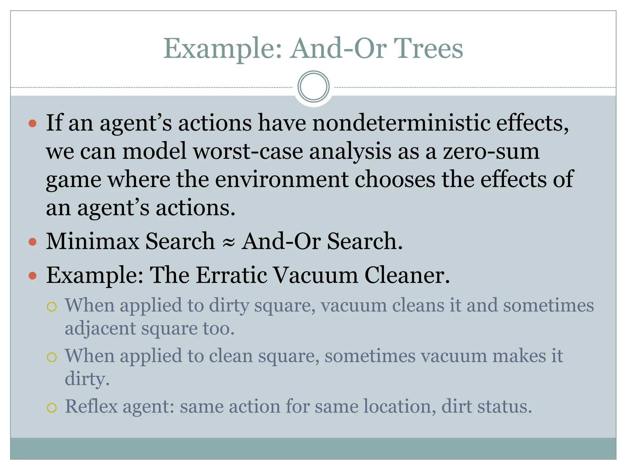
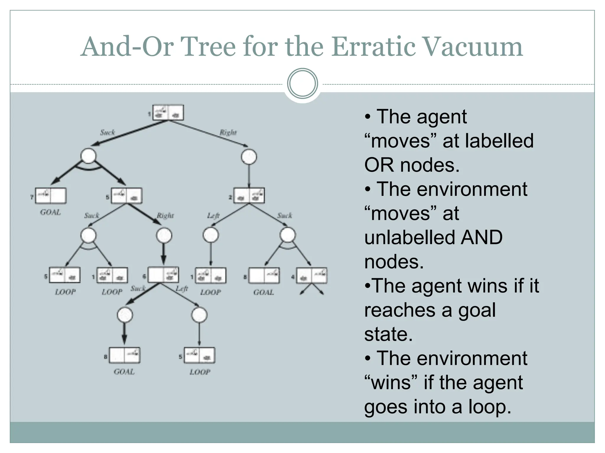
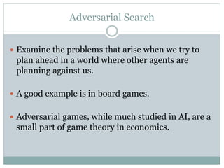
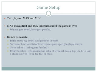
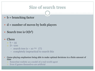
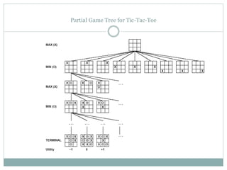
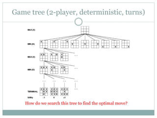
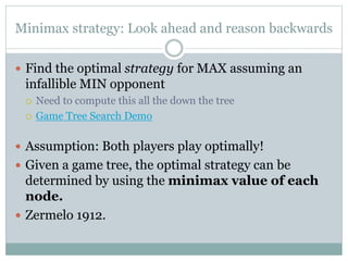
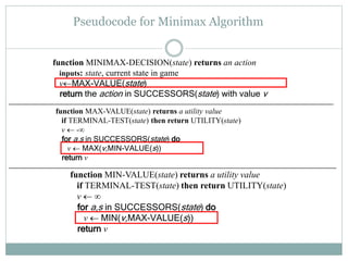
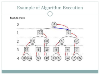
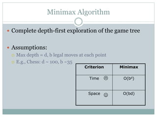
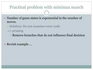
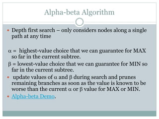
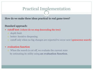
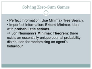
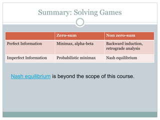
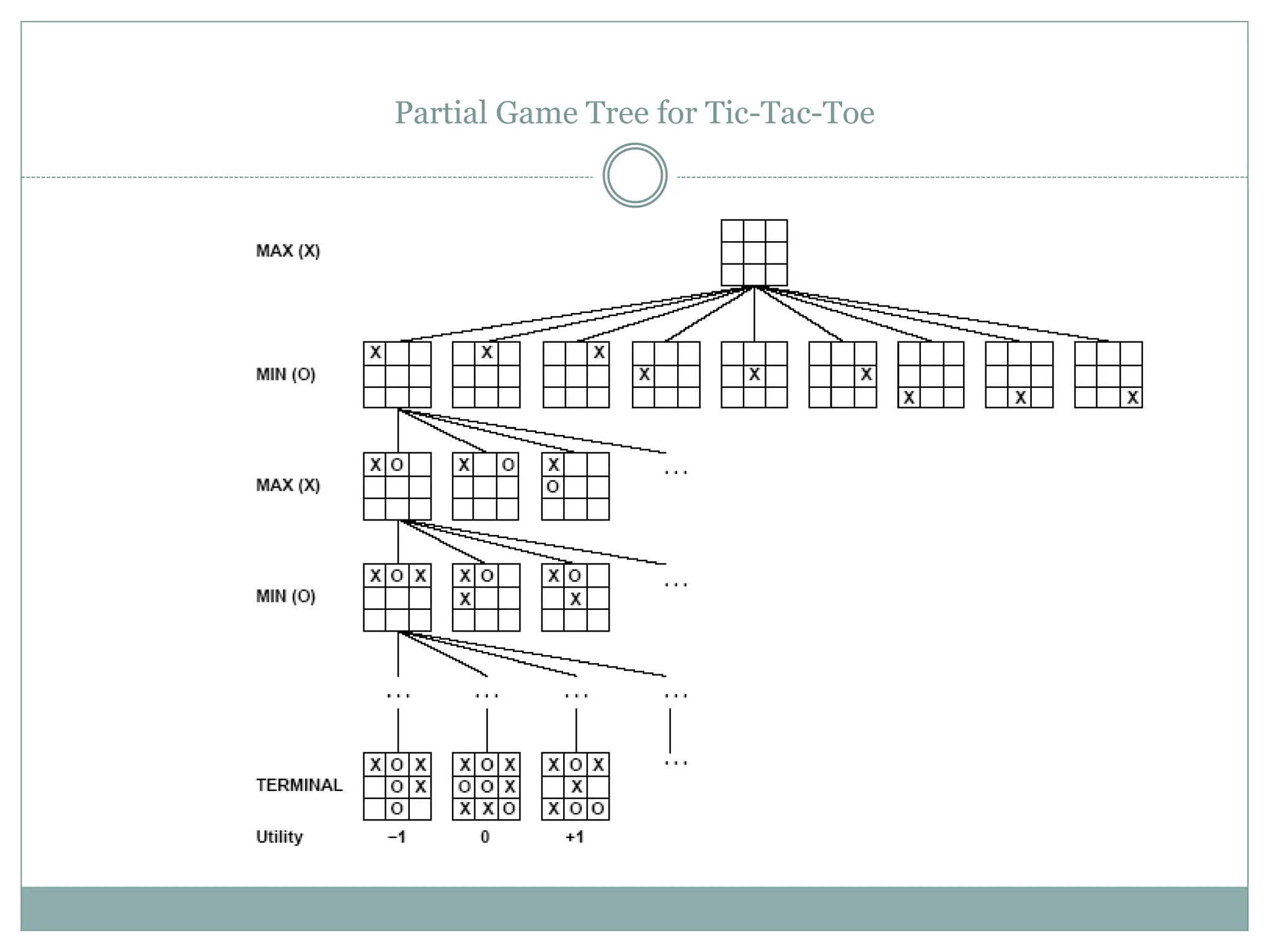
The document discusses adversarial search and game playing in artificial intelligence, focusing on the dynamics of two agents in games like chess and tic-tac-toe. It covers concepts such as minimax strategies, alpha-beta pruning, and evaluation functions, detailing how these techniques allow for optimal decision-making under time constraints. Additionally, it touches on the implications of game theory and how adversarial interactions mirror various multi-agent scenarios, emphasizing the computational challenges associated with simulating game states.

![Alpha-Beta Example
[-∞, +∞]
[-∞,+∞]
Range of possible values
Do DF-search until first leaf](https://image.slidesharecdn.com/mychapter5-240715045141-9c9e0e6f/85/Adversarial-Search-and-Game-Playing-ppt-20-320.jpg)
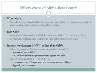
![Alpha-Beta Example (continued)
[-∞,3]
[-∞,+∞]](https://image.slidesharecdn.com/mychapter5-240715045141-9c9e0e6f/85/Adversarial-Search-and-Game-Playing-ppt-21-320.jpg)
![Alpha-Beta Example (continued)
[-∞,3]
[-∞,+∞]](https://image.slidesharecdn.com/mychapter5-240715045141-9c9e0e6f/85/Adversarial-Search-and-Game-Playing-ppt-22-320.jpg)
![Alpha-Beta Example (continued)
[3,+∞]
[3,3]](https://image.slidesharecdn.com/mychapter5-240715045141-9c9e0e6f/85/Adversarial-Search-and-Game-Playing-ppt-23-320.jpg)
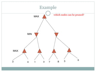
![Alpha-Beta Example (continued)
[-∞,2]
[3,+∞]
[3,3]
This node is worse
for MAX](https://image.slidesharecdn.com/mychapter5-240715045141-9c9e0e6f/85/Adversarial-Search-and-Game-Playing-ppt-24-320.jpg)
![Alpha-Beta Example (continued)
[-∞,2]
[3,14]
[3,3] [-∞,14]
,](https://image.slidesharecdn.com/mychapter5-240715045141-9c9e0e6f/85/Adversarial-Search-and-Game-Playing-ppt-25-320.jpg)
![Alpha-Beta Example (continued)
[−∞,2]
[3,5]
[3,3] [-∞,5]
,](https://image.slidesharecdn.com/mychapter5-240715045141-9c9e0e6f/85/Adversarial-Search-and-Game-Playing-ppt-26-320.jpg)
![Alpha-Beta Example (continued)
[2,2]
[−∞,2]
[3,3]
[3,3]](https://image.slidesharecdn.com/mychapter5-240715045141-9c9e0e6f/85/Adversarial-Search-and-Game-Playing-ppt-27-320.jpg)
![Alpha-Beta Example (continued)
[2,2]
[-∞,2]
[3,3]
[3,3]](https://image.slidesharecdn.com/mychapter5-240715045141-9c9e0e6f/85/Adversarial-Search-and-Game-Playing-ppt-28-320.jpg)
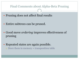
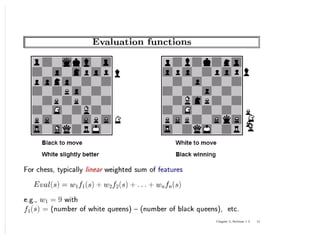
![Static (Heuristic) Evaluation Functions
An Evaluation Function:
estimates how good the current board configuration is for a player.
Typically, one figures how good it is for the player, and how good it is for the
opponent, and subtracts the opponents score from the players
Othello: Number of white pieces - Number of black pieces
Chess: Value of all white pieces - Value of all black pieces
Typical values from -infinity (loss) to +infinity (win) or [-1, +1].
If the board evaluation is X for a player, it’s -X for the opponent.
Many clever ideas about how to use the evaluation function.
e.g. null move heuristic: let opponent move twice.
Example:
Evaluating chess boards,
Checkers
Tic-tac-toe](https://image.slidesharecdn.com/mychapter5-240715045141-9c9e0e6f/85/Adversarial-Search-and-Game-Playing-ppt-34-320.jpg)


![Alpha-Beta Example
[-∞, +∞]
[-∞,+∞]
Range of possible values
Do DF-search until first leaf](https://image.slidesharecdn.com/mychapter5-240715045141-9c9e0e6f/75/Adversarial-Search-and-Game-Playing-ppt-20-2048.jpg)
![Alpha-Beta Example (continued)
[-∞,3]
[-∞,+∞]](https://image.slidesharecdn.com/mychapter5-240715045141-9c9e0e6f/75/Adversarial-Search-and-Game-Playing-ppt-21-2048.jpg)
![Alpha-Beta Example (continued)
[-∞,3]
[-∞,+∞]](https://image.slidesharecdn.com/mychapter5-240715045141-9c9e0e6f/75/Adversarial-Search-and-Game-Playing-ppt-22-2048.jpg)
![Alpha-Beta Example (continued)
[3,+∞]
[3,3]](https://image.slidesharecdn.com/mychapter5-240715045141-9c9e0e6f/75/Adversarial-Search-and-Game-Playing-ppt-23-2048.jpg)
![Alpha-Beta Example (continued)
[-∞,2]
[3,+∞]
[3,3]
This node is worse
for MAX](https://image.slidesharecdn.com/mychapter5-240715045141-9c9e0e6f/75/Adversarial-Search-and-Game-Playing-ppt-24-2048.jpg)
![Alpha-Beta Example (continued)
[-∞,2]
[3,14]
[3,3] [-∞,14]
,](https://image.slidesharecdn.com/mychapter5-240715045141-9c9e0e6f/75/Adversarial-Search-and-Game-Playing-ppt-25-2048.jpg)
![Alpha-Beta Example (continued)
[−∞,2]
[3,5]
[3,3] [-∞,5]
,](https://image.slidesharecdn.com/mychapter5-240715045141-9c9e0e6f/75/Adversarial-Search-and-Game-Playing-ppt-26-2048.jpg)
![Alpha-Beta Example (continued)
[2,2]
[−∞,2]
[3,3]
[3,3]](https://image.slidesharecdn.com/mychapter5-240715045141-9c9e0e6f/75/Adversarial-Search-and-Game-Playing-ppt-27-2048.jpg)
![Alpha-Beta Example (continued)
[2,2]
[-∞,2]
[3,3]
[3,3]](https://image.slidesharecdn.com/mychapter5-240715045141-9c9e0e6f/75/Adversarial-Search-and-Game-Playing-ppt-28-2048.jpg)
![Static (Heuristic) Evaluation Functions
An Evaluation Function:
estimates how good the current board configuration is for a player.
Typically, one figures how good it is for the player, and how good it is for the
opponent, and subtracts the opponents score from the players
Othello: Number of white pieces - Number of black pieces
Chess: Value of all white pieces - Value of all black pieces
Typical values from -infinity (loss) to +infinity (win) or [-1, +1].
If the board evaluation is X for a player, it’s -X for the opponent.
Many clever ideas about how to use the evaluation function.
e.g. null move heuristic: let opponent move twice.
Example:
Evaluating chess boards,
Checkers
Tic-tac-toe](https://image.slidesharecdn.com/mychapter5-240715045141-9c9e0e6f/75/Adversarial-Search-and-Game-Playing-ppt-34-2048.jpg)