Downloaded 605 times

![Bode Plot GM & PM
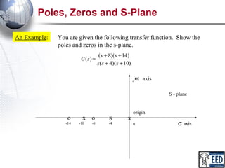
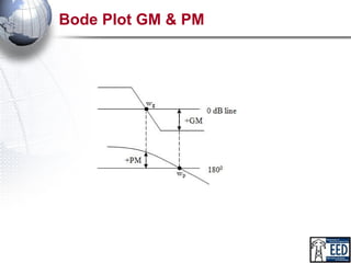
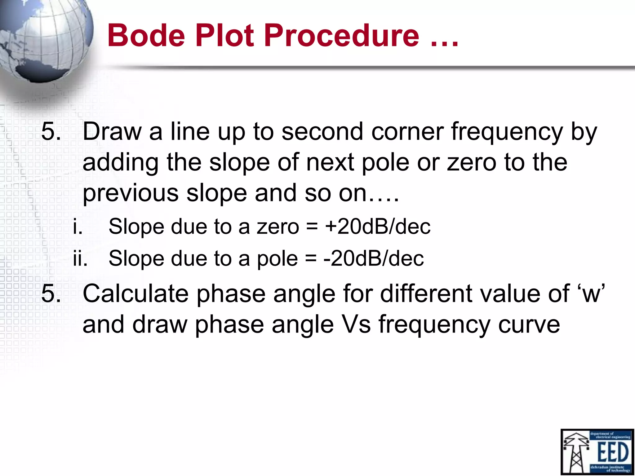
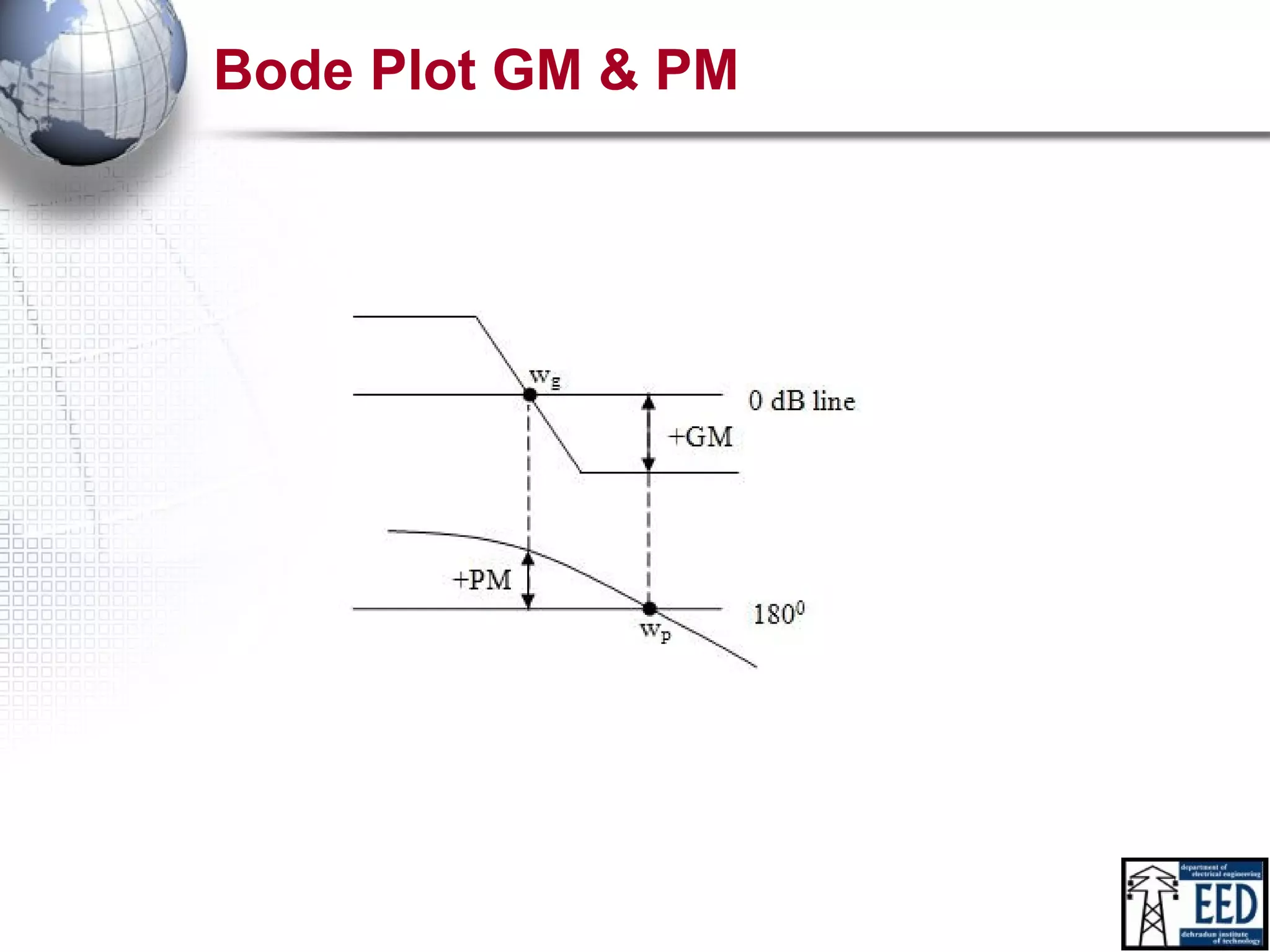
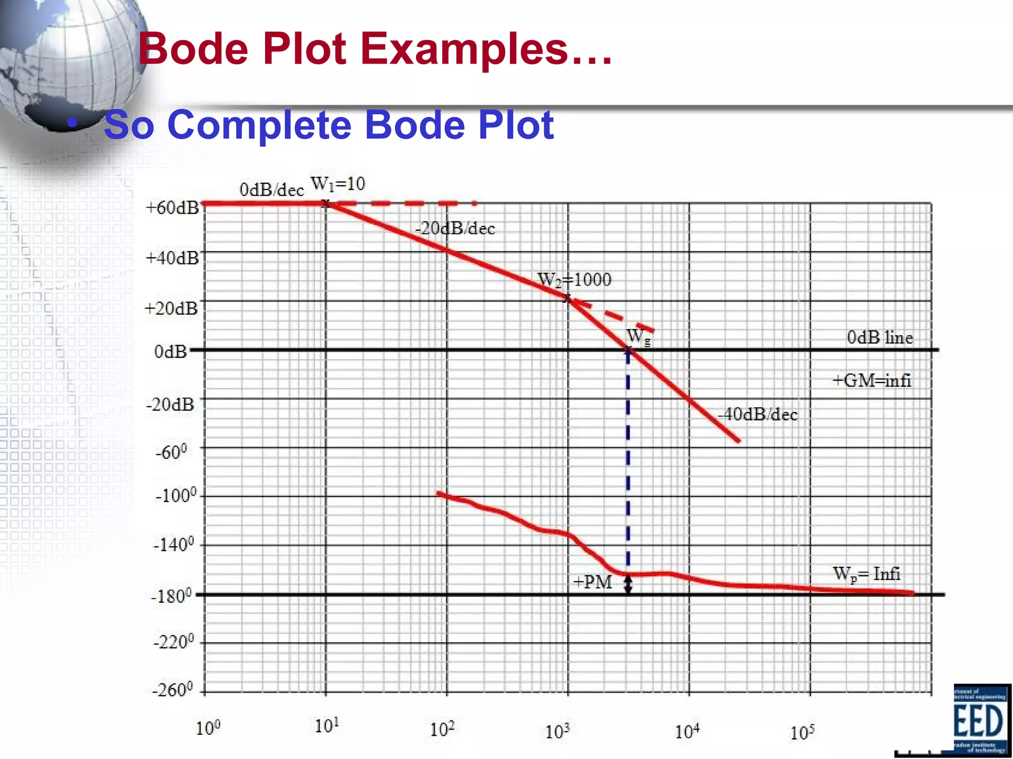
• Gain Margin: It is the amount of gain in db that can be
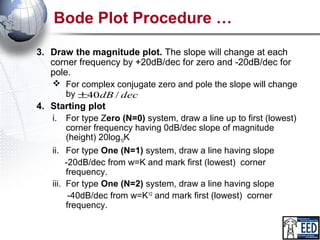
added to the system before the system become
unstable
– GM in dB = 20log10(1/|G(jw|) = -20log10|G(jw|
– Gain cross-over frequency: Frequency where magnitude plot
intersect the 0dB line (x-axis) denoted by wg
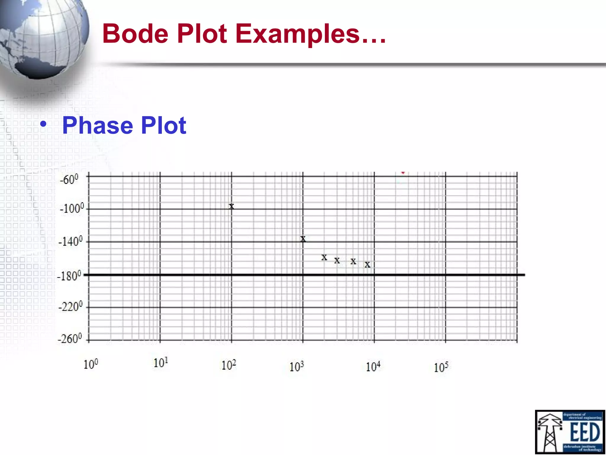
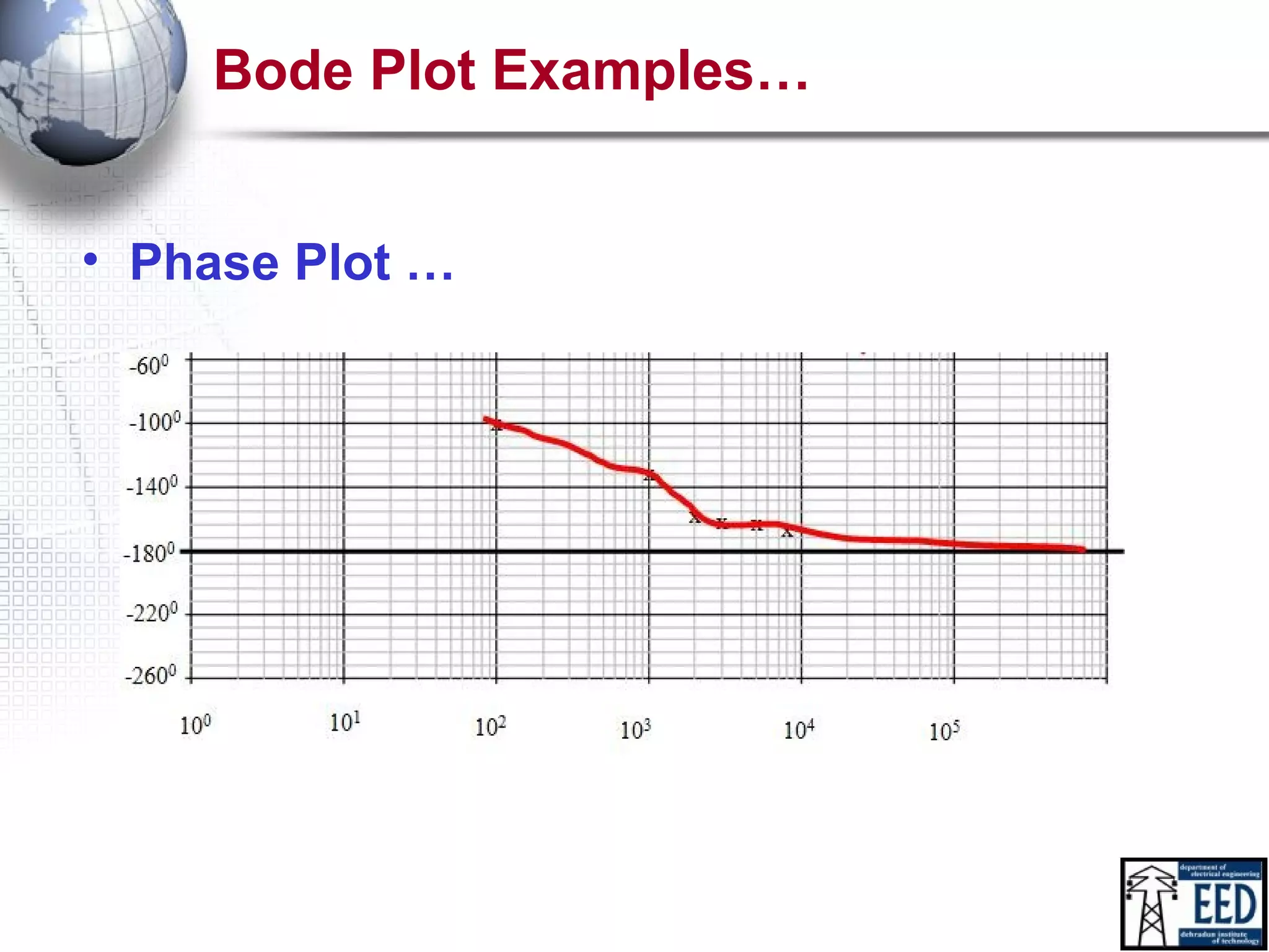
• Phase Margin: It is the amount of phase lag in degree
that can be added to the system before the system
become unstable
– PM in degree = 1800+angle[G(jw)]
– Phase cross-over frequency: Frequency where phase plot
intersect the 1800 dB line (x-axis) denoted by wp
– Less PM => More oscillating system](https://image.slidesharecdn.com/notestee602bodeplot-141201003423-conversion-gate01/85/bode_plot-By-DEV-12-320.jpg)


![Bode Plot GM & PM
• Gain Margin: It is the amount of gain in db that can be
added to the system before the system become
unstable
– GM in dB = 20log10(1/|G(jw|) = -20log10|G(jw|
– Gain cross-over frequency: Frequency where magnitude plot
intersect the 0dB line (x-axis) denoted by wg
• Phase Margin: It is the amount of phase lag in degree
that can be added to the system before the system
become unstable
– PM in degree = 1800+angle[G(jw)]
– Phase cross-over frequency: Frequency where phase plot
intersect the 1800 dB line (x-axis) denoted by wp
– Less PM => More oscillating system](https://image.slidesharecdn.com/notestee602bodeplot-141201003423-conversion-gate01/75/bode_plot-By-DEV-12-2048.jpg)
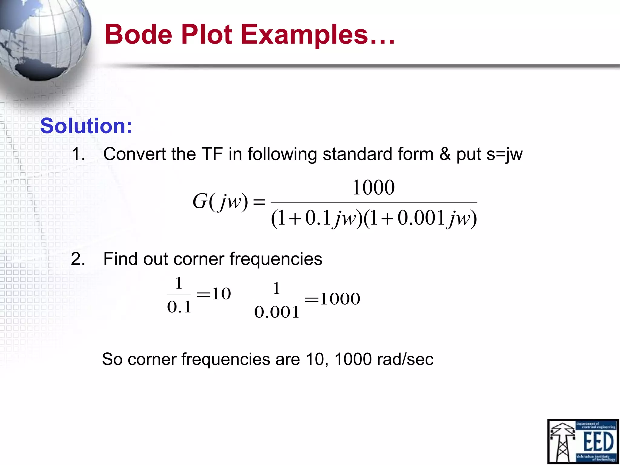


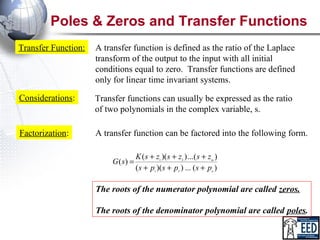
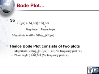
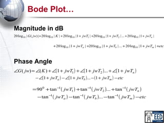
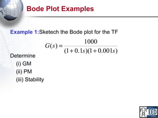
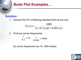
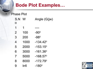
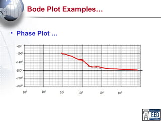
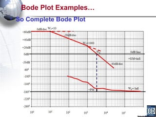
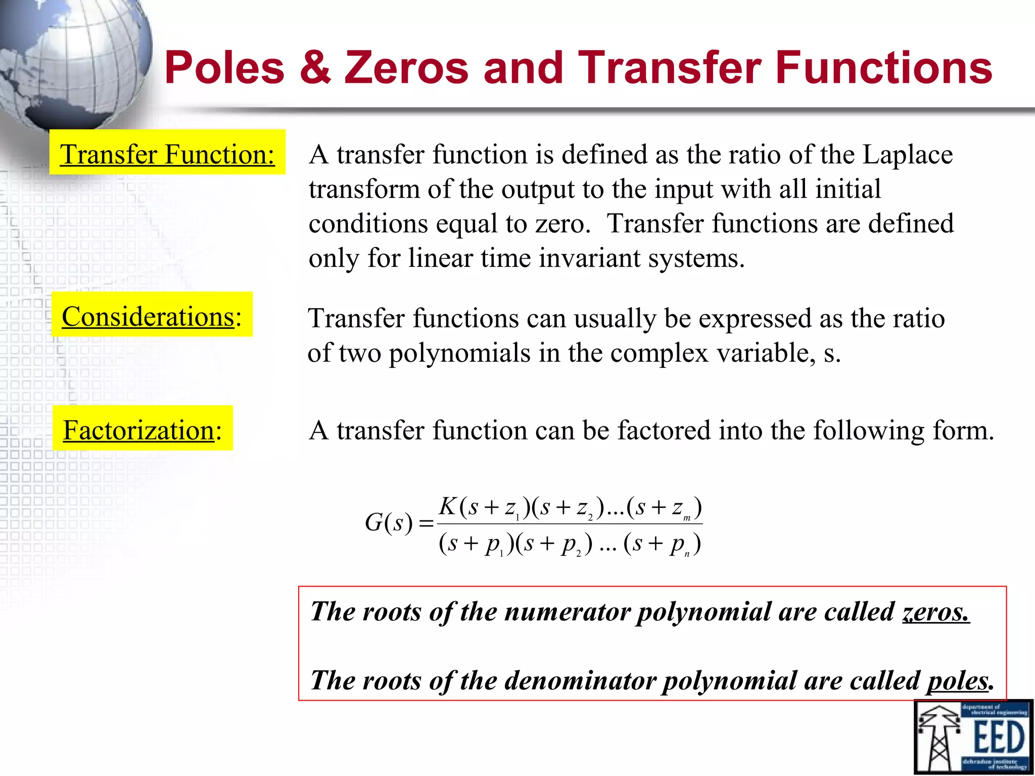
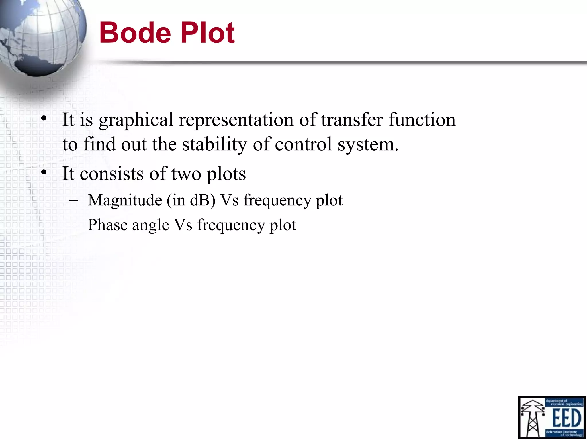
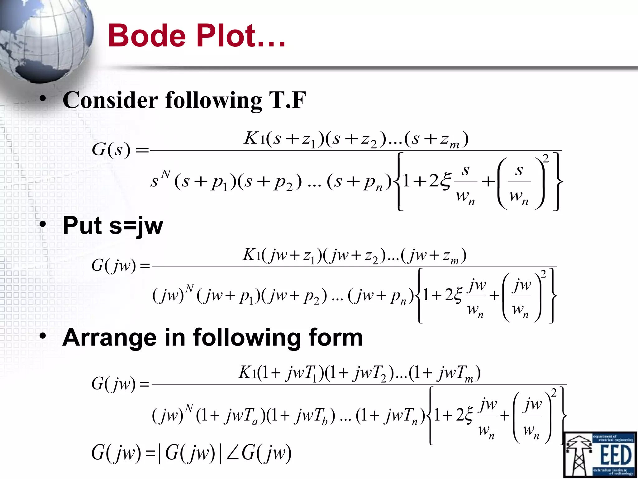
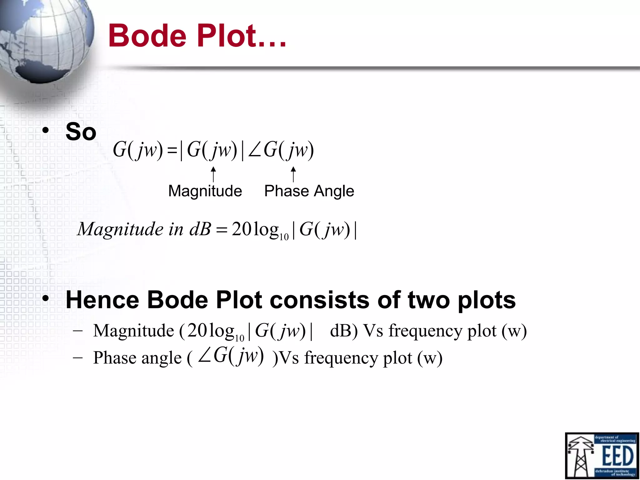
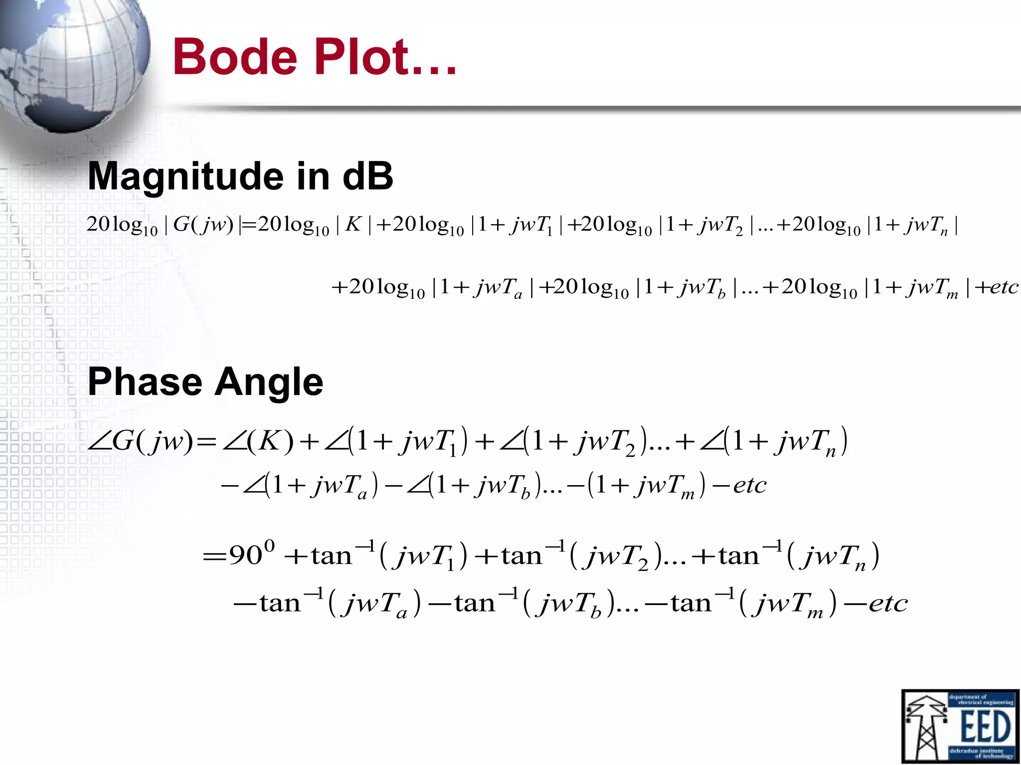
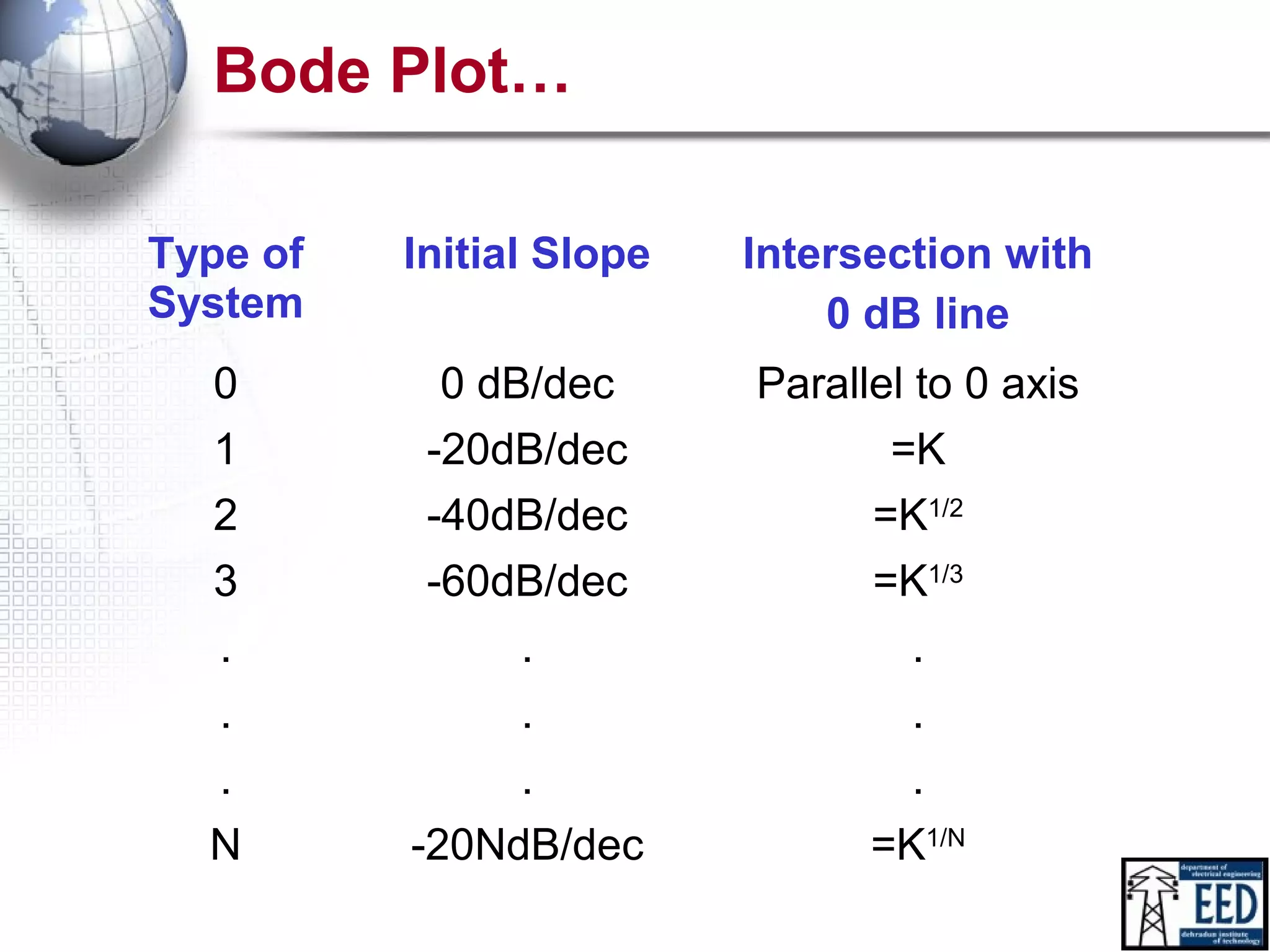
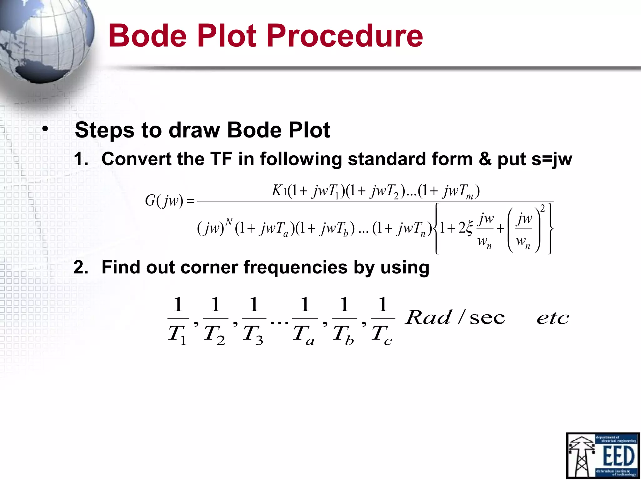
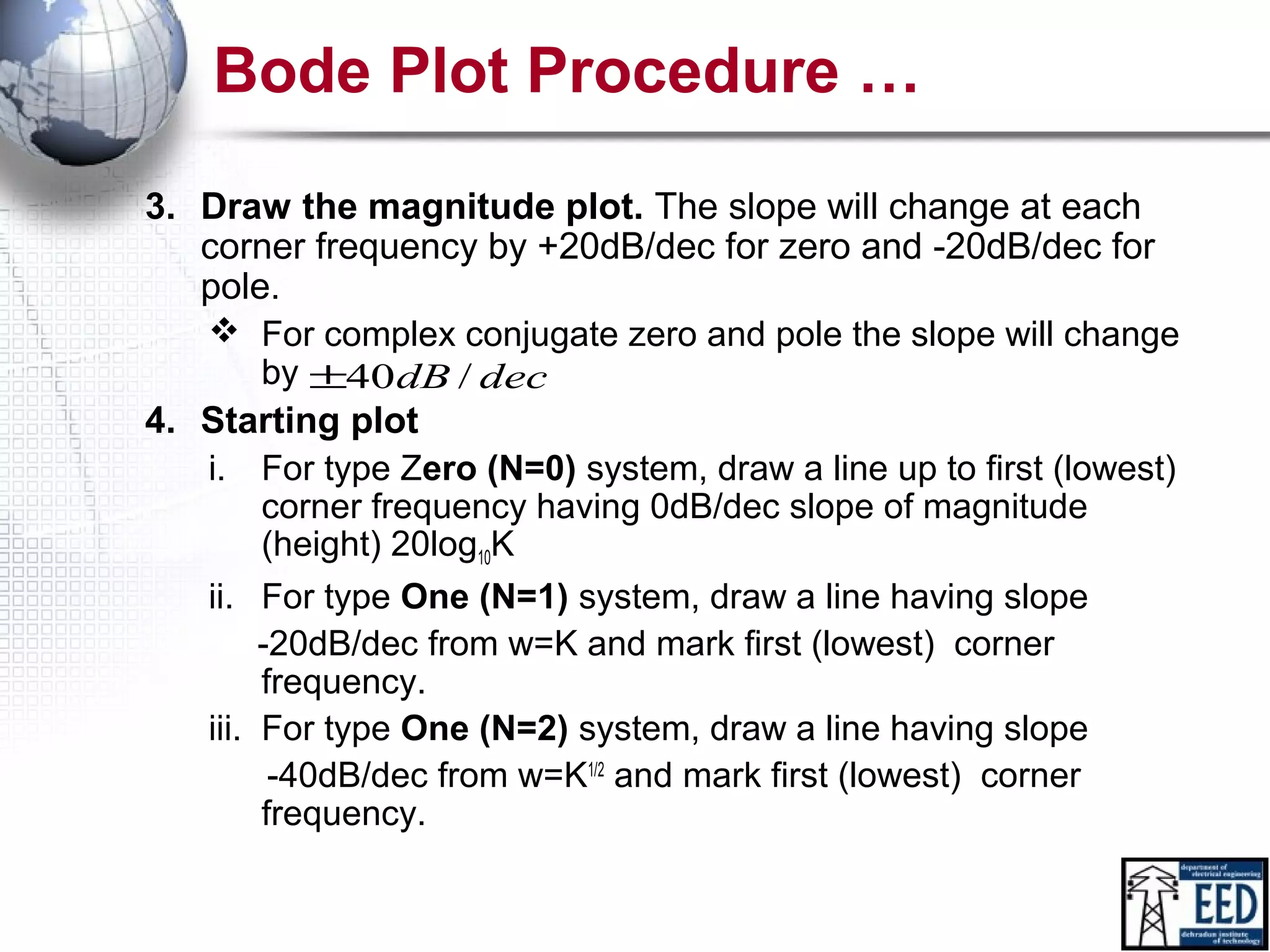
This document discusses Bode plots, which are used to analyze the stability of linear time-invariant control systems. Bode plots graphically represent a system's transfer function and consist of a magnitude plot and a phase plot versus frequency. The magnitude plot shows the gain in decibels and the phase plot shows the phase angle. Together these plots can determine the gain and phase margins of a system, which indicate its stability. Examples are provided to demonstrate how to construct Bode plots from transfer functions and analyze system stability.


![Circuit Network Analysis - [Chapter5] Transfer function, frequency response, ...](https://cdn.slidesharecdn.com/ss_thumbnails/ch5-150613063859-lva1-app6891-thumbnail.jpg?width=600ounds&width=560&fit=bounds)
![Circuit Network Analysis - [Chapter4] Laplace Transform](https://cdn.slidesharecdn.com/ss_thumbnails/ch4-150613063858-lva1-app6891-thumbnail.jpg?width=600ounds&width=560&fit=bounds)


