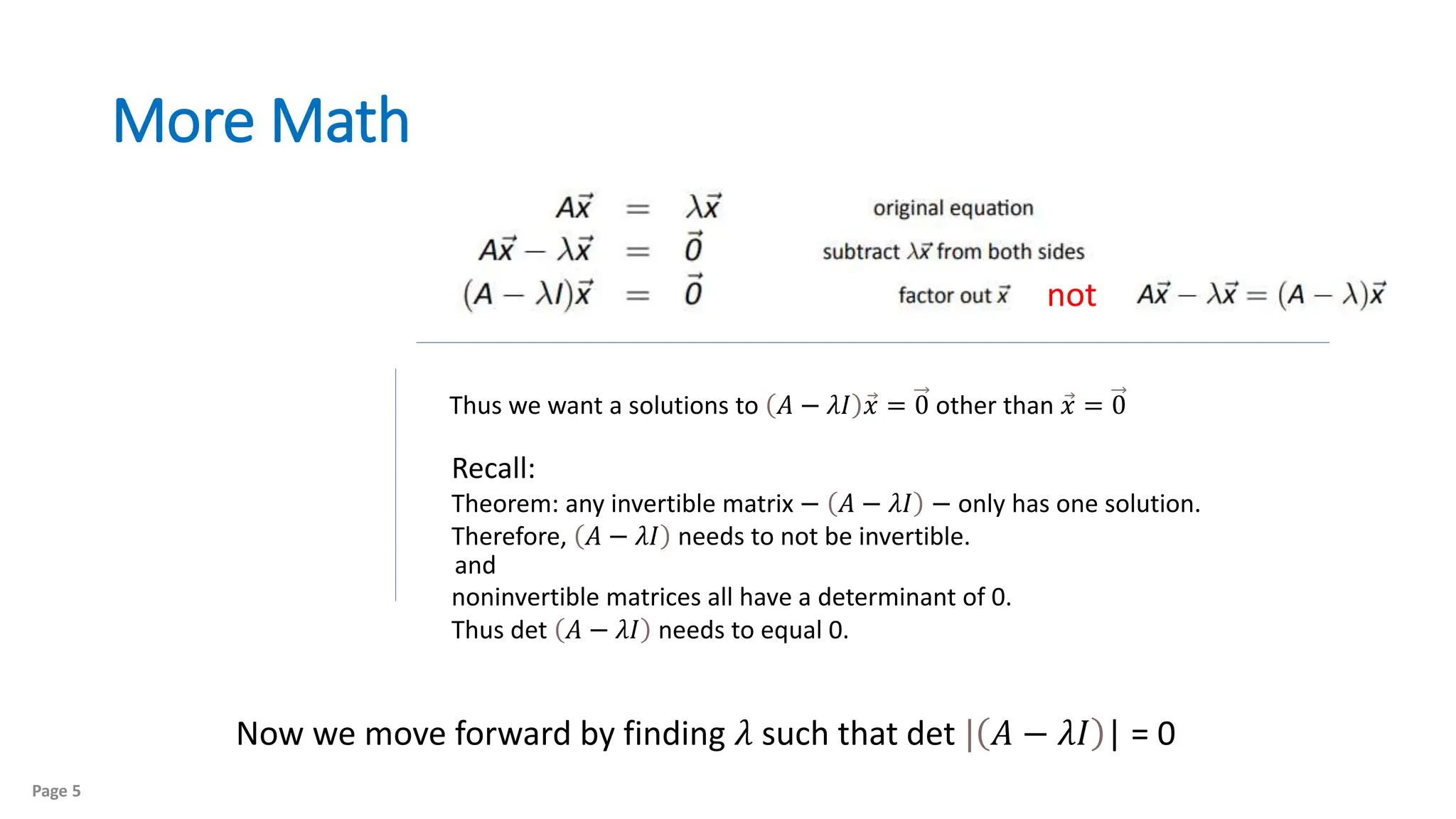
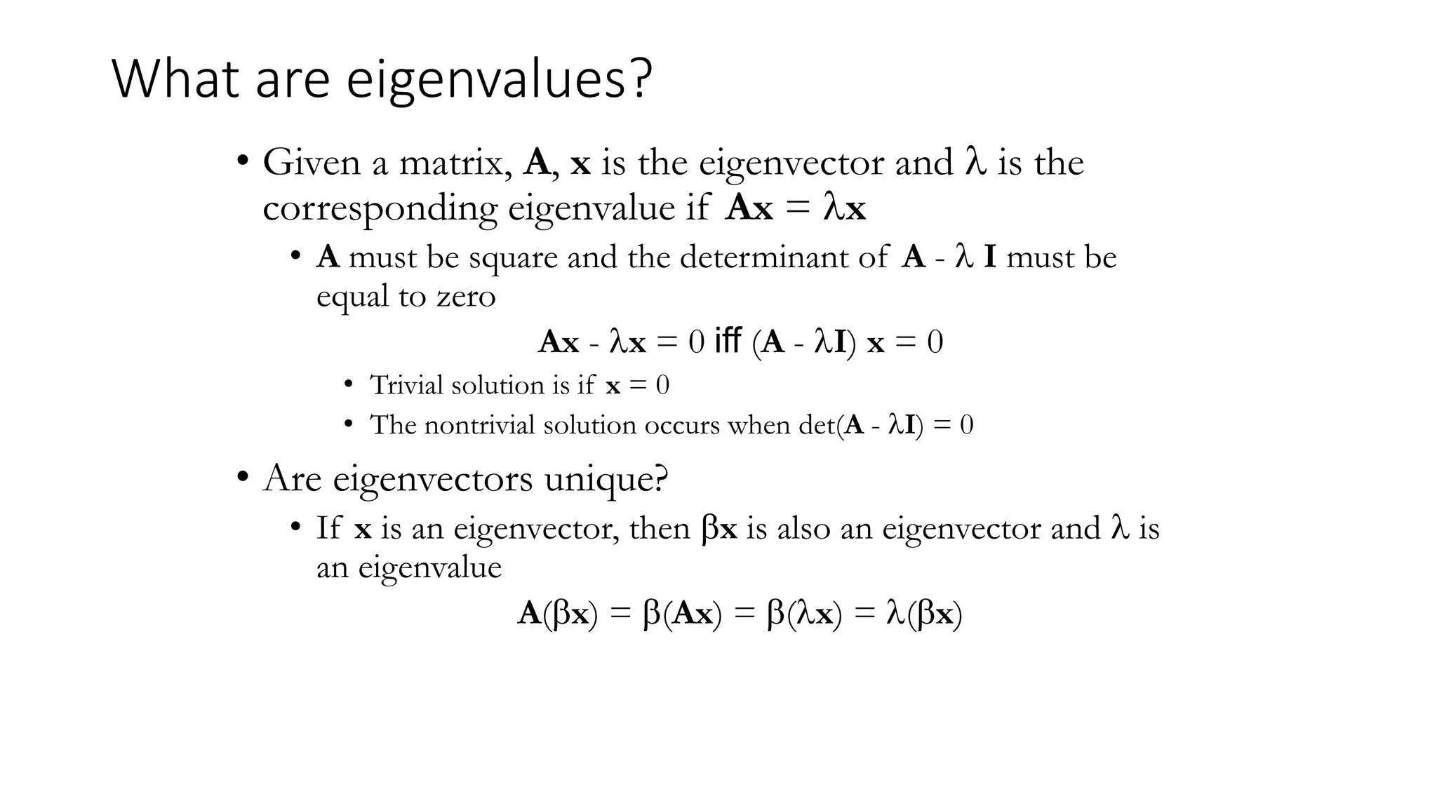
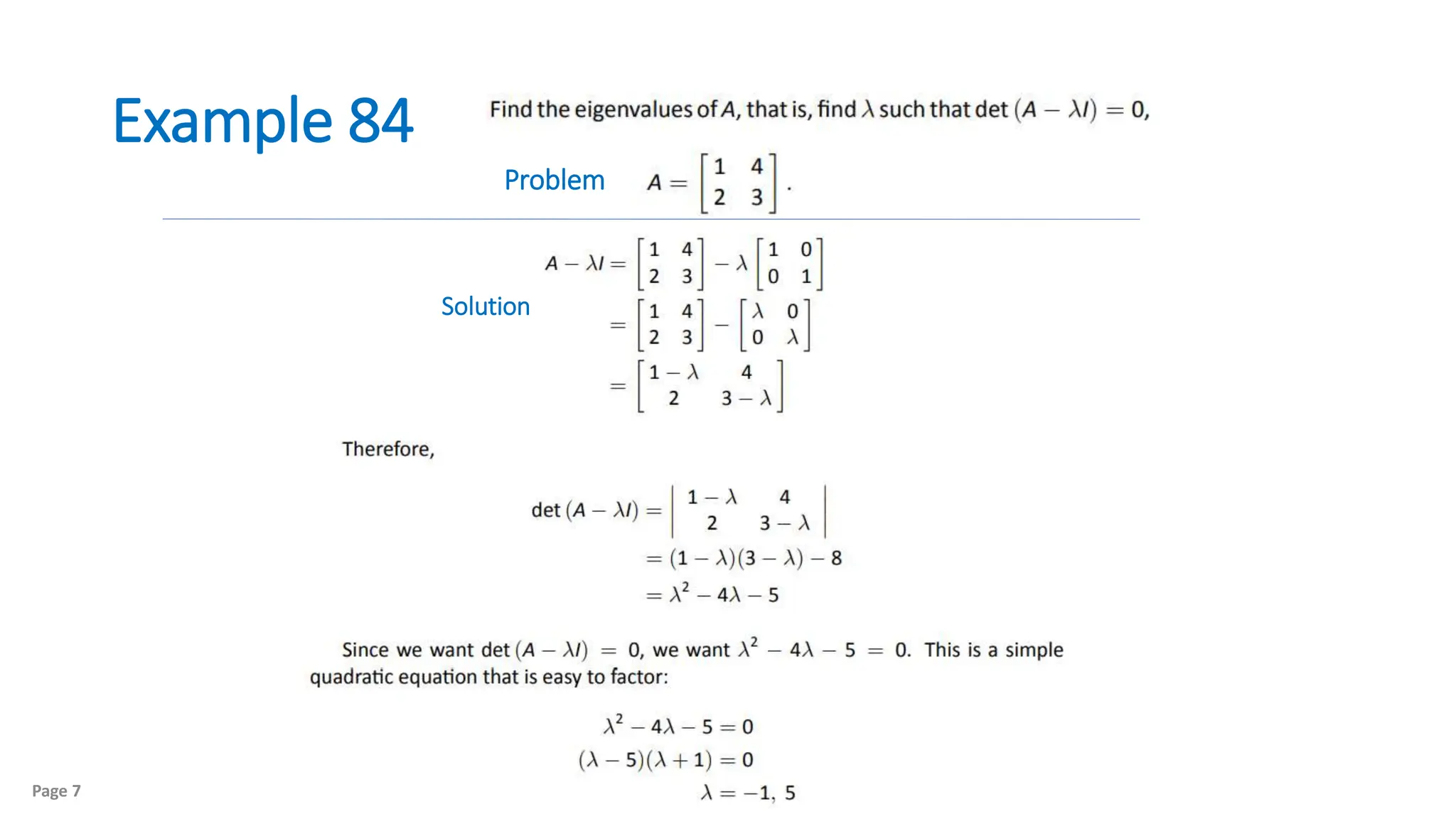
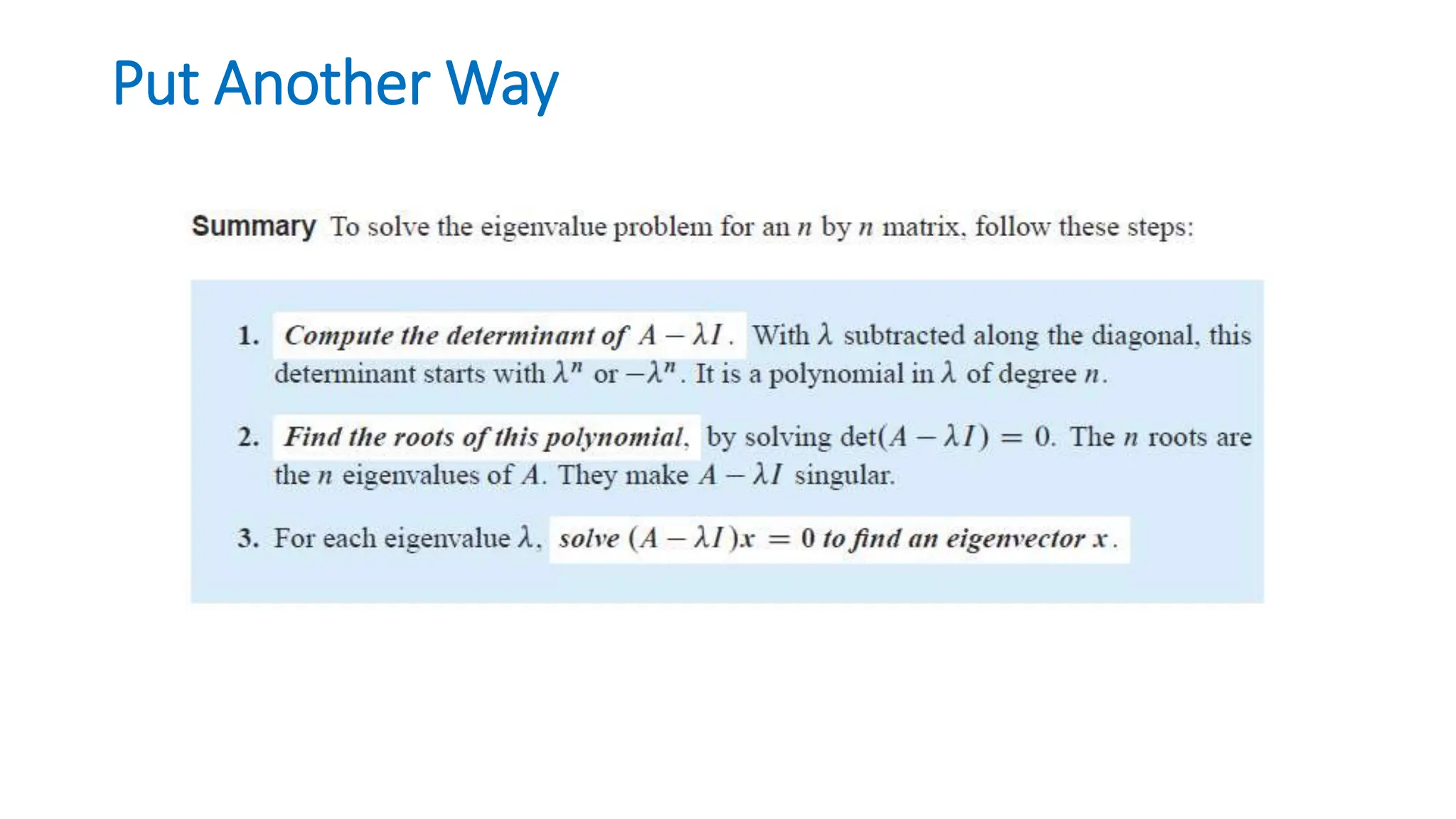
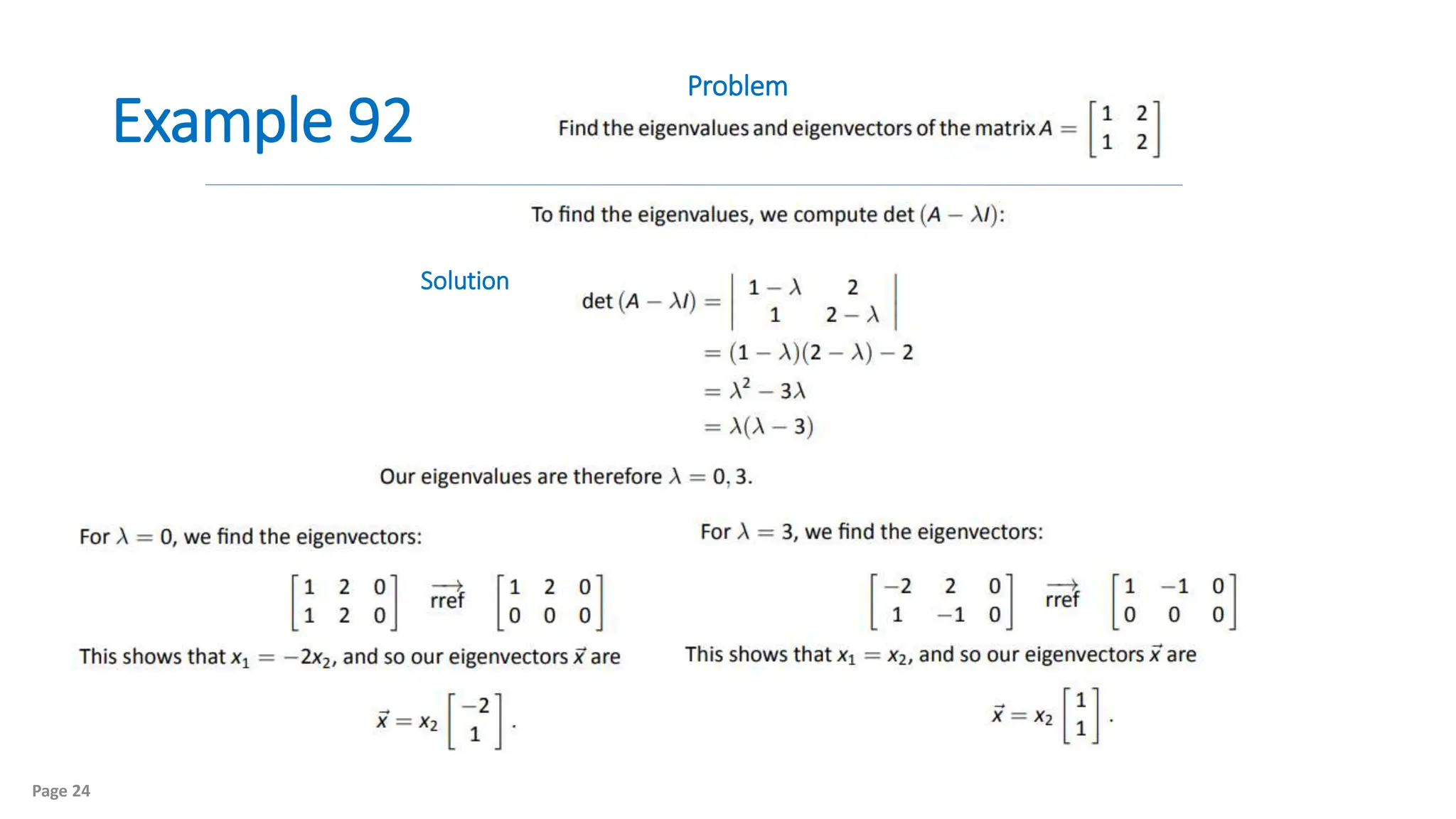
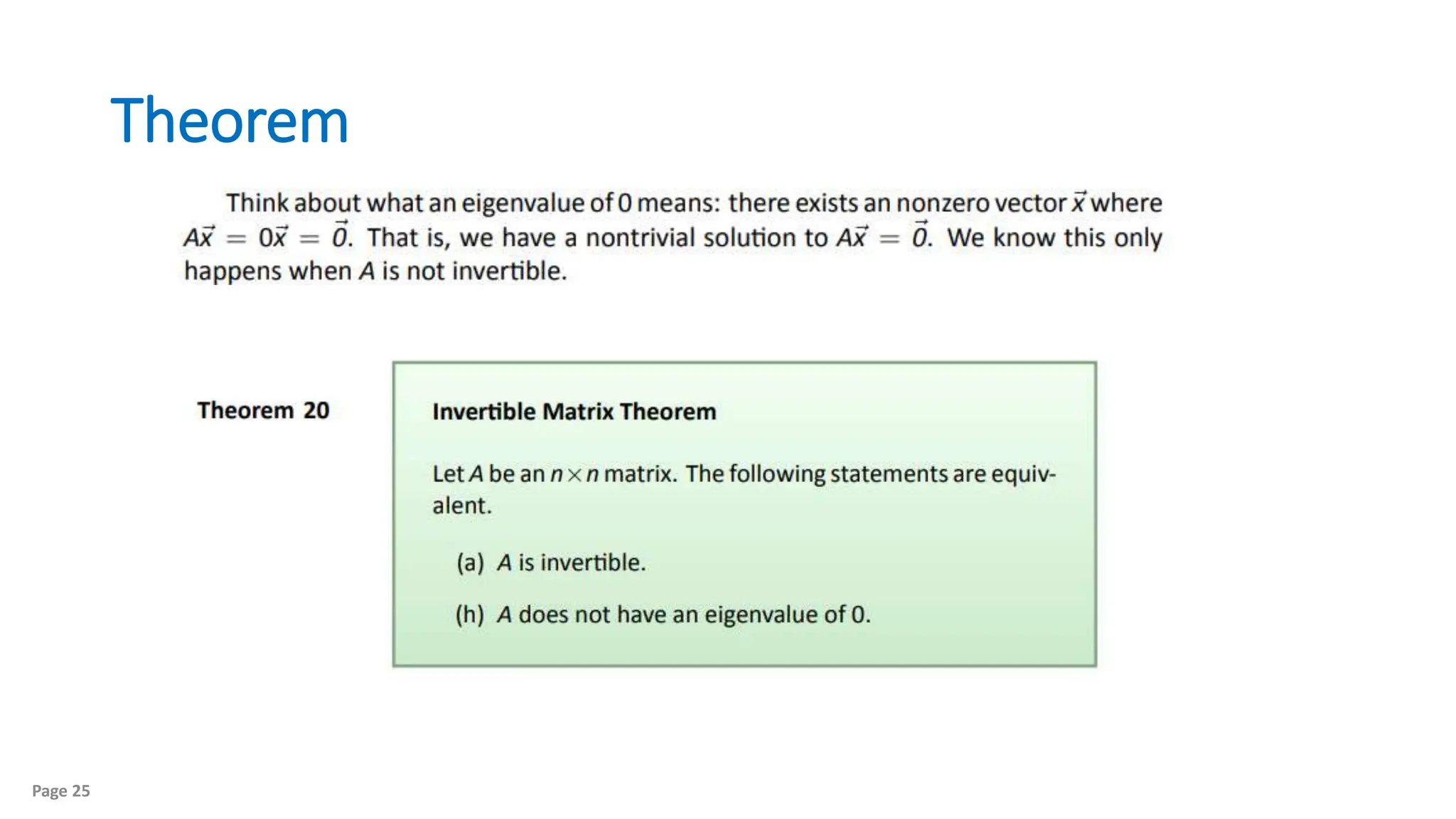
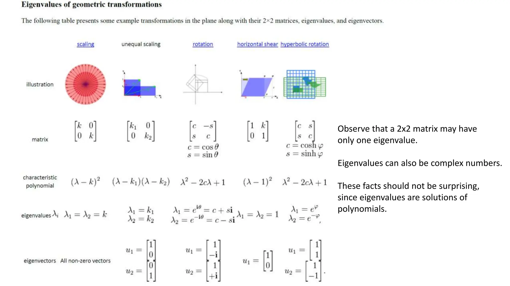
KEMBAR78
Chapter 4 EIgen values and eigen vectors.pptx
Chapter 4
Fundamentals of Matrix Algebra By Gregory Hartman
Do we ever have the case where where a is some scalar?
Central Question
4.1 Eigenvalues and
Eigenvectors
Predefinition Workup
Page 3
Page 4
More Math
Page 5
not
Thus we want a solutions to 𝐴 − 𝜆𝐼 𝑥 = 0 other than 𝑥 = 0
Recall:
Theorem: any invertible matrix − 𝐴 − 𝜆𝐼 − only has one solution.
Therefore, 𝐴 − 𝜆𝐼 needs to not be invertible.
noninvertible matrices all have a determinant of 0.
Thus det 𝐴 − 𝜆𝐼 needs to equal 0.
Now we move forward by finding 𝜆 such that det | 𝐴 − 𝜆𝐼 | = 0
and
What are eigenvalues?
• Given a matrix, A, x is the eigenvector and  is the
corresponding eigenvalue if Ax = x
• A must be square and the determinant of A -  I must be
equal to zero
Ax - x = 0 iff (A - I) x = 0
• Trivial solution is if x = 0
• The nontrivial solution occurs when det(A - I) = 0
• Are eigenvectors unique?
• If x is an eigenvector, then x is also an eigenvector and  is
an eigenvalue
A(x) = (Ax) = (x) = (x)
Example 84
Page 7
Solution
Problem
Example 85
Page 8
Problem
Solution
Calculating the Eigenvectors/values
• Expand the det(A - I) = 0 for a 2 x 2 matrix
• For a 2 x 2 matrix, this is a simple quadratic equation with two solutions
(maybe complex)
• This “characteristic equation” can be used to solve for x
 
  
    0
0
0
det
0
1
0
0
1
det
det
21
12
22
11
22
11
2
21
12
22
11
22
21
12
11
22
21
12
11











































a
a
a
a
a
a
a
a
a
a
a
a
a
a
a
a
a
a
I
A








   
 
21
12
22
11
2
22
11
22
11
4 a
a
a
a
a
a
a
a






Eigenvalue example
• Consider,
• The corresponding eigenvectors can be computed as
• For  = 0, one possible solution is x = (2, -1)
• For  = 5, one possible solution is x = (1, 2)
   
 






























5
,
0
)
4
1
(
0
2
2
4
1
)
4
1
(
0
4
2
2
1
2
2
21
12
22
11
22
11
2







 a
a
a
a
a
a
A

























































































































0
0
1
2
2
4
1
2
2
4
0
5
0
0
5
4
2
2
1
5
0
0
4
2
2
1
4
2
2
1
0
0
0
0
0
4
2
2
1
0
y
x
y
x
y
x
y
x
y
x
y
x
y
x
y
x


Definition
Page 11
Key Idea
Page 12
Put Another Way
Example 86
Page 14
Fine the eigenvalues of A, and for each eigenvalue, find an eigenvector where
Solution
Problem
Example 86
Page 15
Fine the eigenvalues of A, and for each eigenvalue, find an eigenvector where
Solution
Problem
Example 86
Page 16
Fine the eigenvalues of A, and for each eigenvalue, find an eigenvector where
Solution
Problem
Summary
Example 86
Page 17
Fine the eigenvalues of A, and for each eigenvalue, find an eigenvector where
Solution
Problem
4.2 Properties of Eigenvalues
and Eigenvectors
Page 19
Note regarding section material: matrices with a trace of 0 are important.
Example 90
Page 20
Solution
Problem
Page 21
The Eigenvectors and Eigenvalues of A and A-1
If 𝜆 is an eigenvalue of A, then 1/𝜆 is an eigenvalue of A-1.
The corresponding eigenvectors are the same.
Page 22
The Eigenvectors and Eigenvalues of A and AT
The Eigenvalues of A and AT are the same, but eigenvectors are different.
Page 23
Page 24
Example 92
Problem
Solution
Page 25
Theorem
Observe that a 2x2 matrix may have
only one eigenvalue.
Eigenvalues can also be complex numbers.
These facts should not be surprising,
since eigenvalues are solutions of
polynomials.
Page 27
Finding Eigenvalues in Real Applications
The eigenvalues of a matrix A can be determined by finding the roots of the characteristic polynomial. Explicit
algebraic formulas for the roots of a polynomial exist only if the degree n is 4 or less. Therefore, for matrices of
order 5 or more, the eigenvalues and eigenvectors cannot be obtained by an explicit algebraic formula and must
be computed by approximate numerical methods.
We would expect that for larger matrices a computer would be used to factor the characteristic polynomials. In
reality, this method is unreliable as roundoff errors cause unpredictable results. Furthermore, before computing
the characteristic polynomial, we need to compute the determinant, also a very expensive process. Efficient,
accurate methods to compute eigenvalues and eigenvectors of arbitrary matrices were not known until the
advent of the QR algorithm in 1961.
Question: how then are eigenvalues found?
Answer: Via iterative processes that transform matrix A into a matrix that is almost an upper triangular
matrix. The more iterations, the better approximation.
Once the value of an eigenvalue is known, the corresponding eigenvectors can be found by finding non-zero
solutions of the eigenvalue equation, that becomes a system of linear equations with known coefficients.
Page 28
Example Compute the eigenvalues and eigenvectors for matrix A. How about A2 , A-1 , and A + 4I ?
𝐴 =
2 −1
−1 2

Chapter 4 EIgen values and eigen vectors.pptx

  • 1.
    Chapter 4 Fundamentals ofMatrix Algebra By Gregory Hartman Do we ever have the case where where a is some scalar? Central Question
  • 2.
  • 3.
  • 4.
  • 5.
    More Math Page 5 not Thuswe want a solutions to 𝐴 − 𝜆𝐼 𝑥 = 0 other than 𝑥 = 0 Recall: Theorem: any invertible matrix − 𝐴 − 𝜆𝐼 − only has one solution. Therefore, 𝐴 − 𝜆𝐼 needs to not be invertible. noninvertible matrices all have a determinant of 0. Thus det 𝐴 − 𝜆𝐼 needs to equal 0. Now we move forward by finding 𝜆 such that det | 𝐴 − 𝜆𝐼 | = 0 and
  • 6.
    What are eigenvalues? •Given a matrix, A, x is the eigenvector and  is the corresponding eigenvalue if Ax = x • A must be square and the determinant of A -  I must be equal to zero Ax - x = 0 iff (A - I) x = 0 • Trivial solution is if x = 0 • The nontrivial solution occurs when det(A - I) = 0 • Are eigenvectors unique? • If x is an eigenvector, then x is also an eigenvector and  is an eigenvalue A(x) = (Ax) = (x) = (x)
  • 7.
  • 8.
  • 9.
    Calculating the Eigenvectors/values •Expand the det(A - I) = 0 for a 2 x 2 matrix • For a 2 x 2 matrix, this is a simple quadratic equation with two solutions (maybe complex) • This “characteristic equation” can be used to solve for x          0 0 0 det 0 1 0 0 1 det det 21 12 22 11 22 11 2 21 12 22 11 22 21 12 11 22 21 12 11                                            a a a a a a a a a a a a a a a a a a I A               21 12 22 11 2 22 11 22 11 4 a a a a a a a a      
  • 10.
    Eigenvalue example • Consider, •The corresponding eigenvectors can be computed as • For  = 0, one possible solution is x = (2, -1) • For  = 5, one possible solution is x = (1, 2)                                     5 , 0 ) 4 1 ( 0 2 2 4 1 ) 4 1 ( 0 4 2 2 1 2 2 21 12 22 11 22 11 2         a a a a a a A                                                                                                                          0 0 1 2 2 4 1 2 2 4 0 5 0 0 5 4 2 2 1 5 0 0 4 2 2 1 4 2 2 1 0 0 0 0 0 4 2 2 1 0 y x y x y x y x y x y x y x y x  
  • 11.
  • 12.
  • 13.
  • 14.
    Example 86 Page 14 Finethe eigenvalues of A, and for each eigenvalue, find an eigenvector where Solution Problem
  • 15.
    Example 86 Page 15 Finethe eigenvalues of A, and for each eigenvalue, find an eigenvector where Solution Problem
  • 16.
    Example 86 Page 16 Finethe eigenvalues of A, and for each eigenvalue, find an eigenvector where Solution Problem Summary
  • 17.
    Example 86 Page 17 Finethe eigenvalues of A, and for each eigenvalue, find an eigenvector where Solution Problem
  • 19.
    4.2 Properties ofEigenvalues and Eigenvectors Page 19 Note regarding section material: matrices with a trace of 0 are important.
  • 20.
  • 21.
    Page 21 The Eigenvectorsand Eigenvalues of A and A-1 If 𝜆 is an eigenvalue of A, then 1/𝜆 is an eigenvalue of A-1. The corresponding eigenvectors are the same.
  • 22.
    Page 22 The Eigenvectorsand Eigenvalues of A and AT The Eigenvalues of A and AT are the same, but eigenvectors are different.
  • 23.
  • 24.
  • 25.
  • 26.
    Observe that a2x2 matrix may have only one eigenvalue. Eigenvalues can also be complex numbers. These facts should not be surprising, since eigenvalues are solutions of polynomials.
  • 27.
    Page 27 Finding Eigenvaluesin Real Applications The eigenvalues of a matrix A can be determined by finding the roots of the characteristic polynomial. Explicit algebraic formulas for the roots of a polynomial exist only if the degree n is 4 or less. Therefore, for matrices of order 5 or more, the eigenvalues and eigenvectors cannot be obtained by an explicit algebraic formula and must be computed by approximate numerical methods. We would expect that for larger matrices a computer would be used to factor the characteristic polynomials. In reality, this method is unreliable as roundoff errors cause unpredictable results. Furthermore, before computing the characteristic polynomial, we need to compute the determinant, also a very expensive process. Efficient, accurate methods to compute eigenvalues and eigenvectors of arbitrary matrices were not known until the advent of the QR algorithm in 1961. Question: how then are eigenvalues found? Answer: Via iterative processes that transform matrix A into a matrix that is almost an upper triangular matrix. The more iterations, the better approximation. Once the value of an eigenvalue is known, the corresponding eigenvectors can be found by finding non-zero solutions of the eigenvalue equation, that becomes a system of linear equations with known coefficients.
  • 28.
    Page 28 Example Computethe eigenvalues and eigenvectors for matrix A. How about A2 , A-1 , and A + 4I ? 𝐴 = 2 −1 −1 2