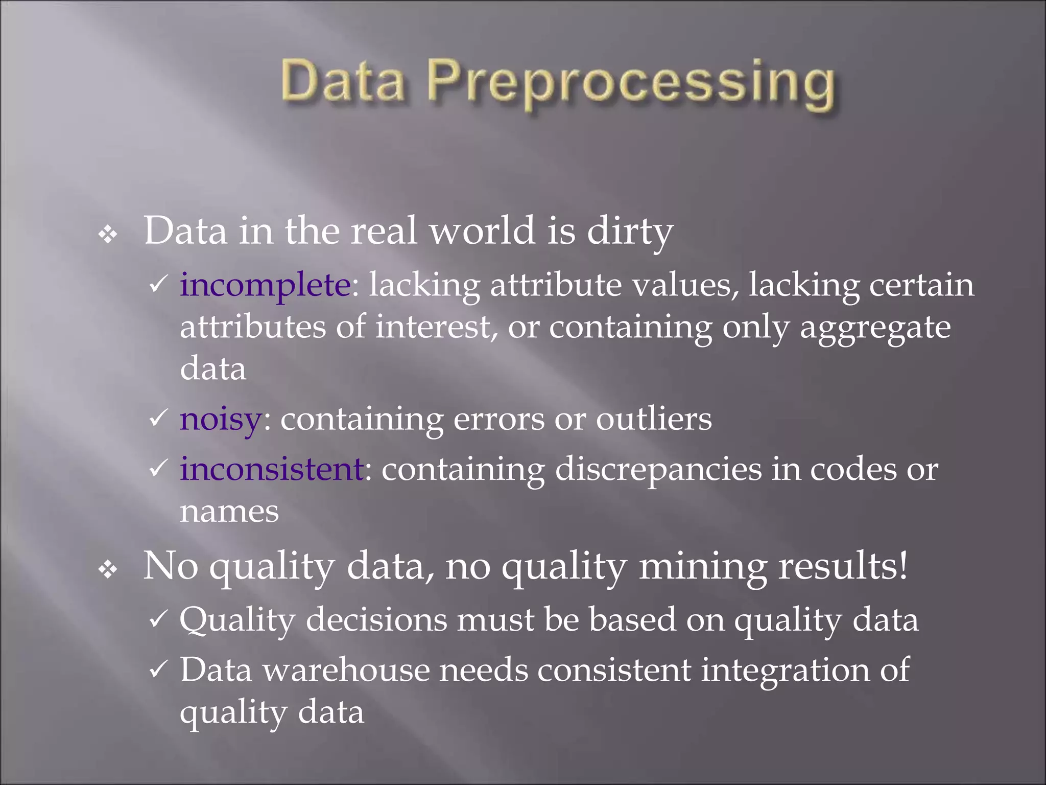
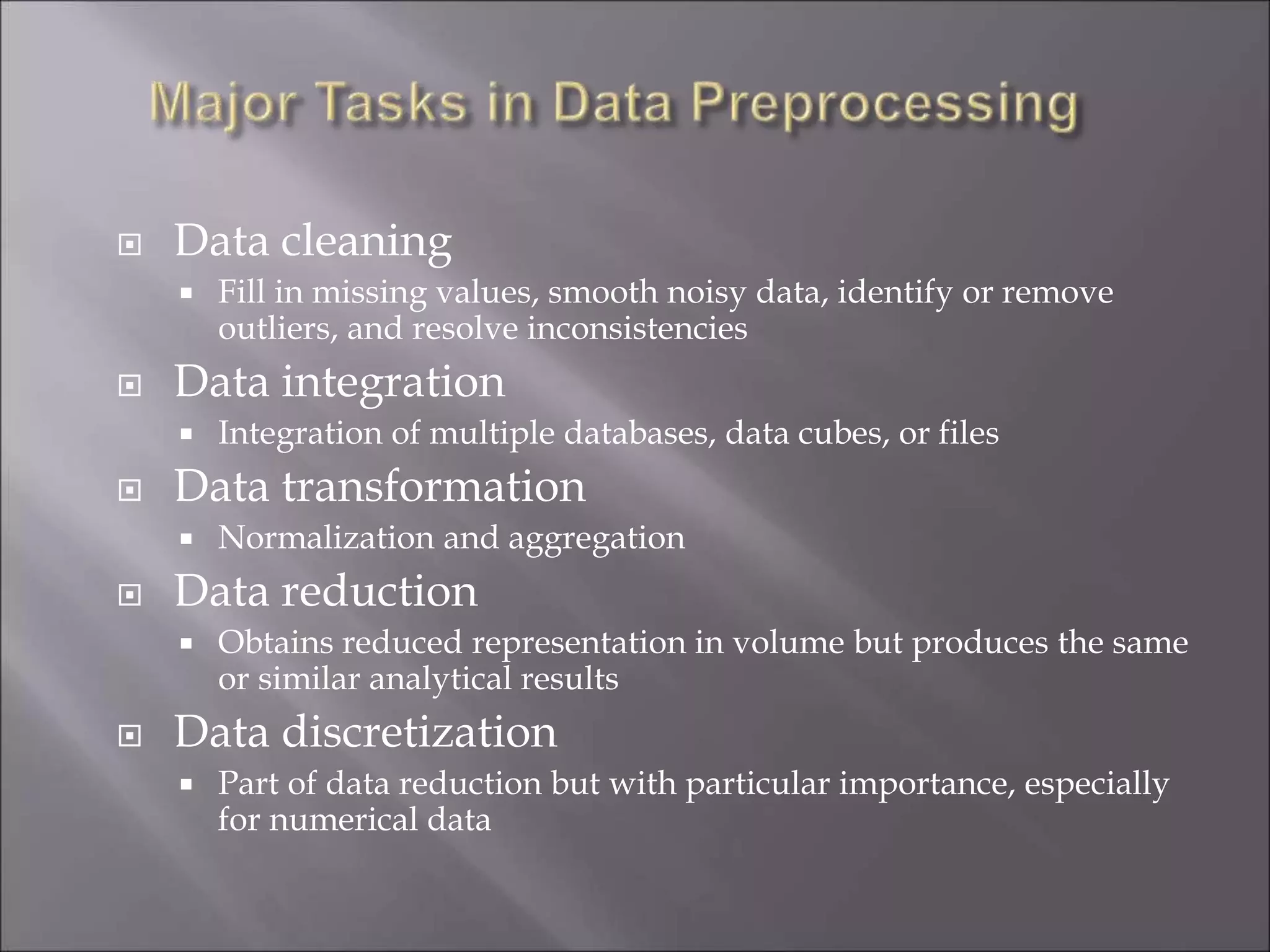
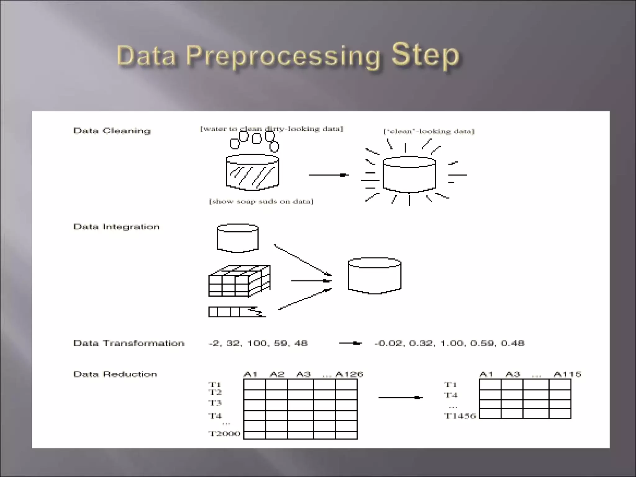
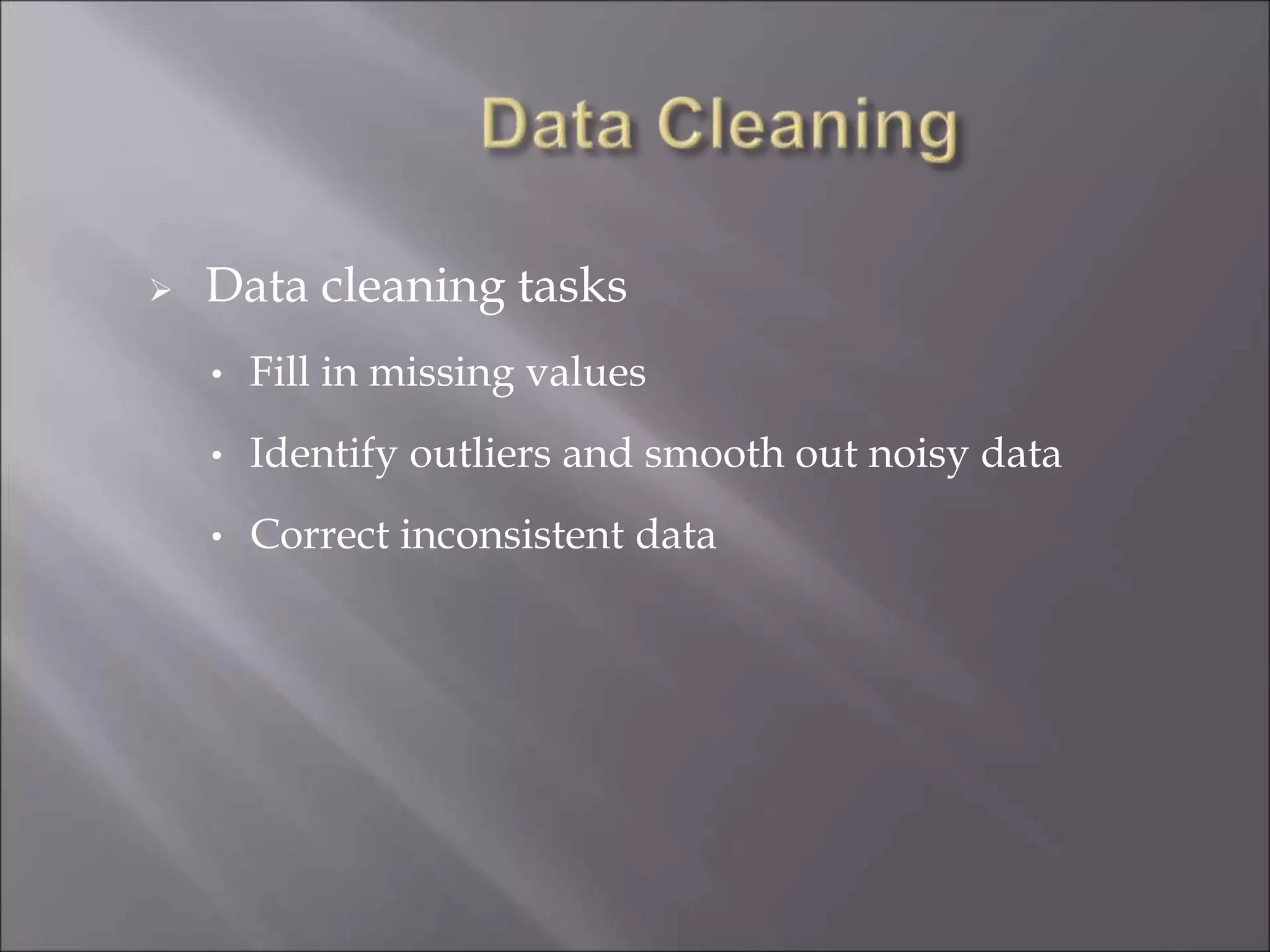
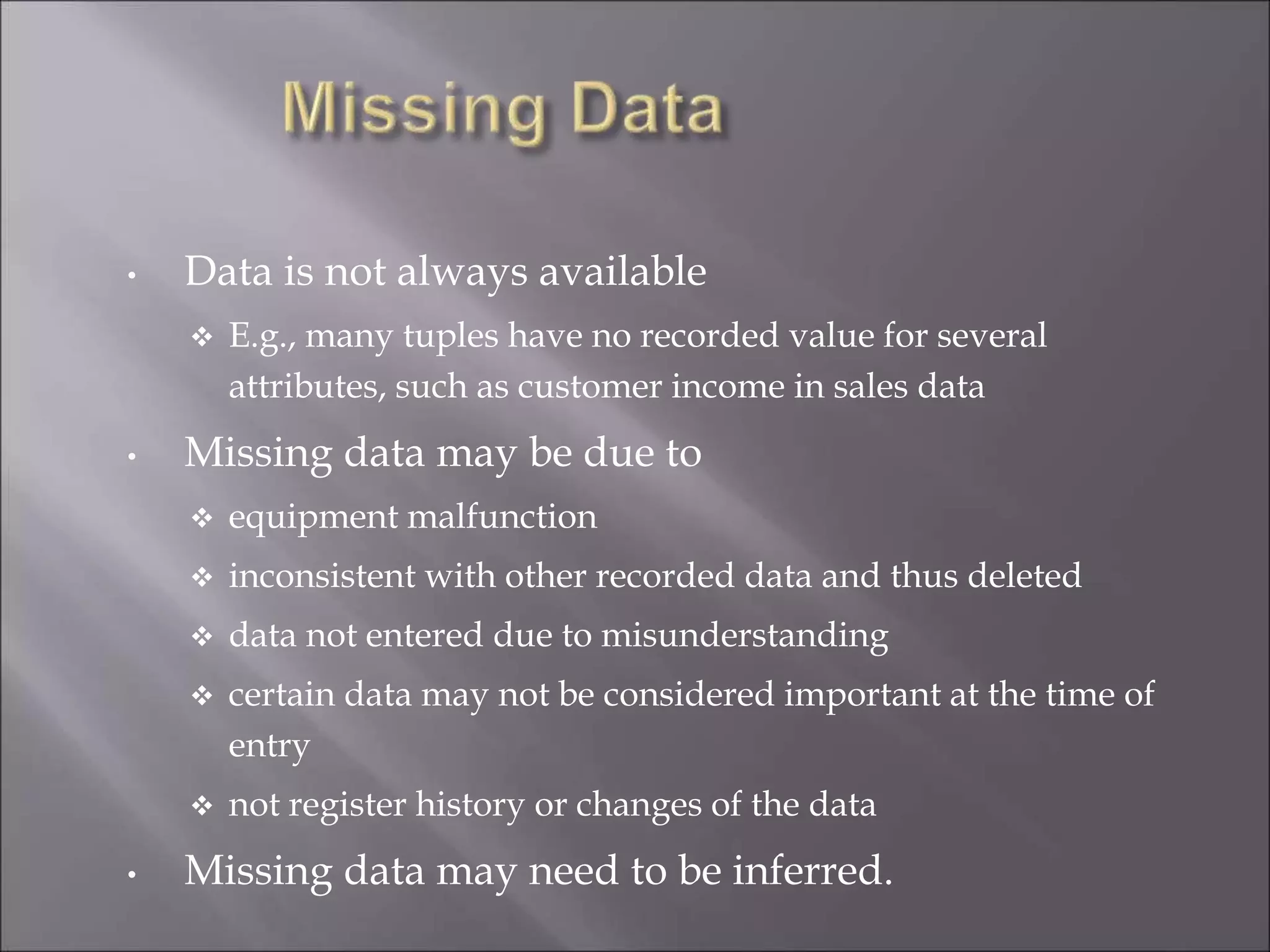
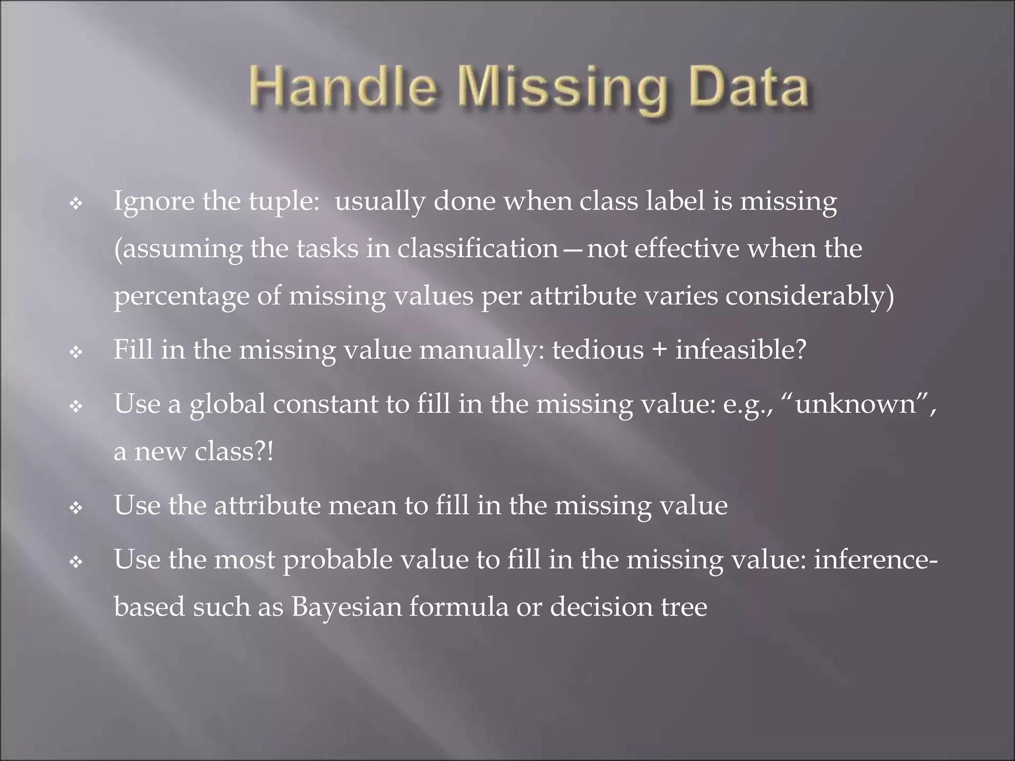
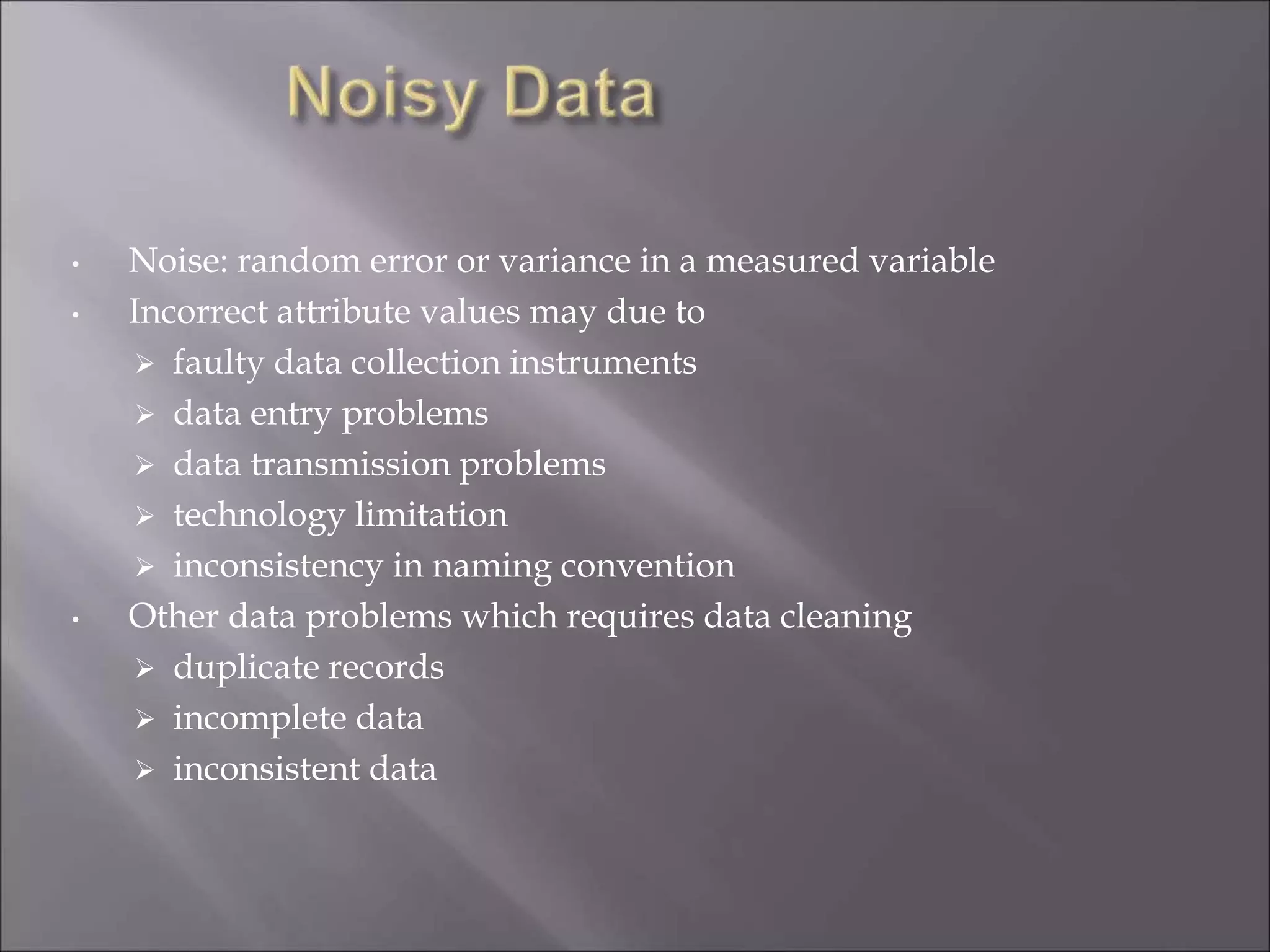
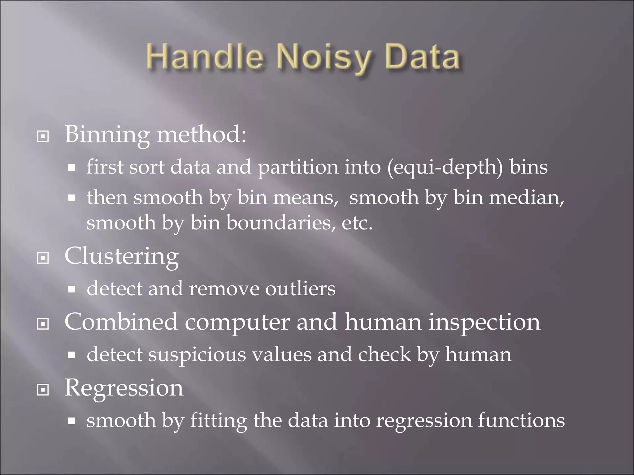
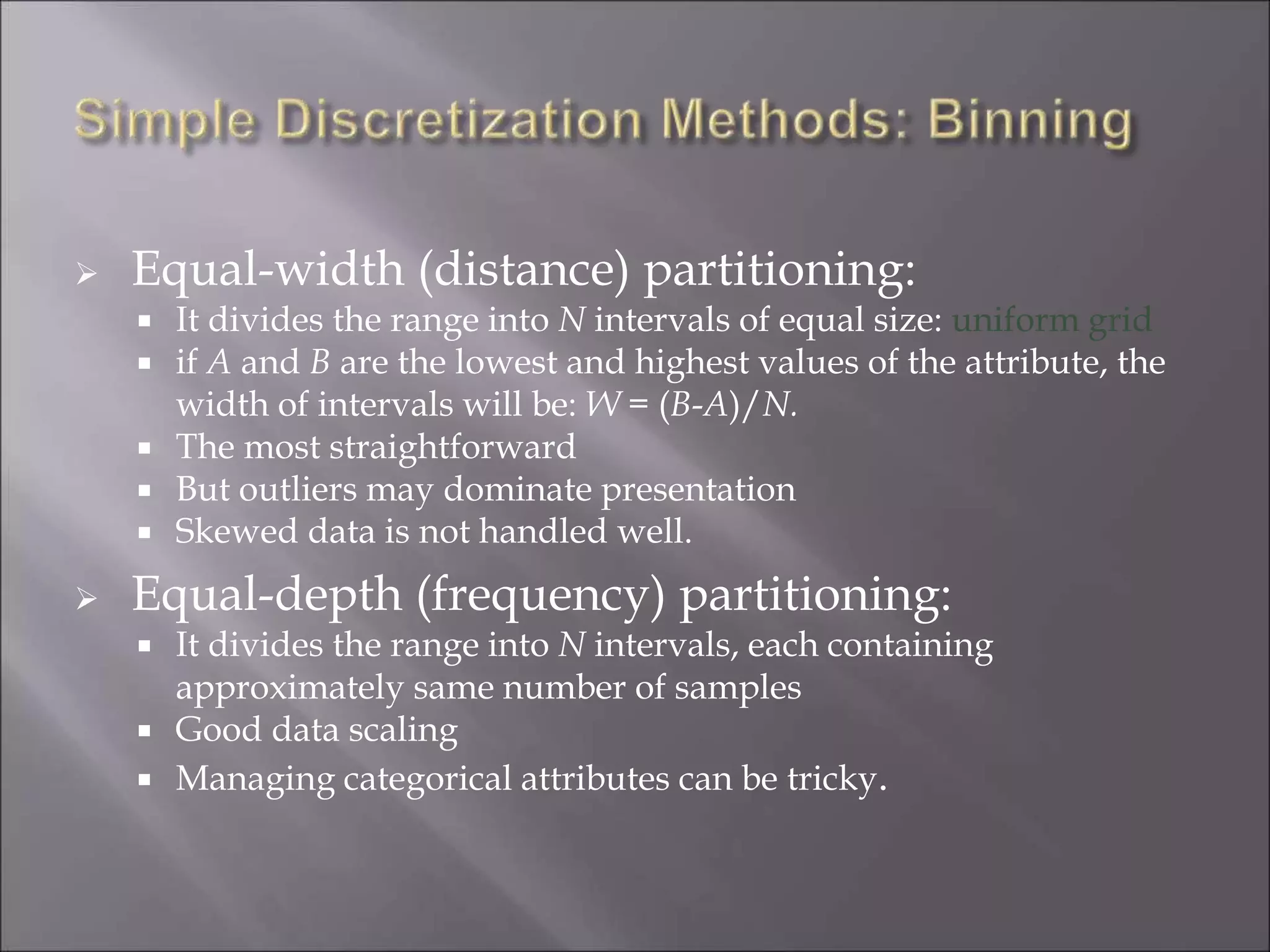
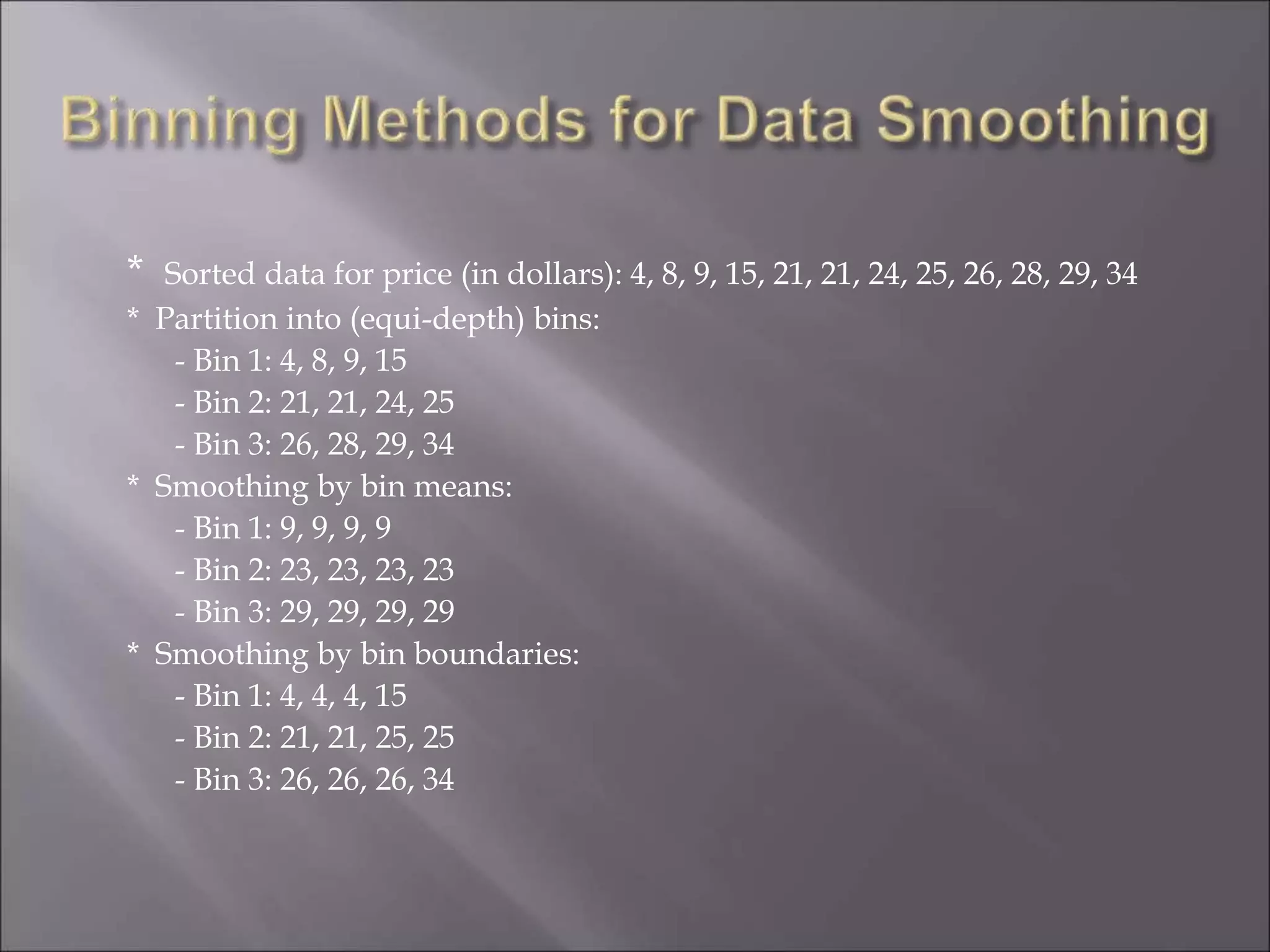
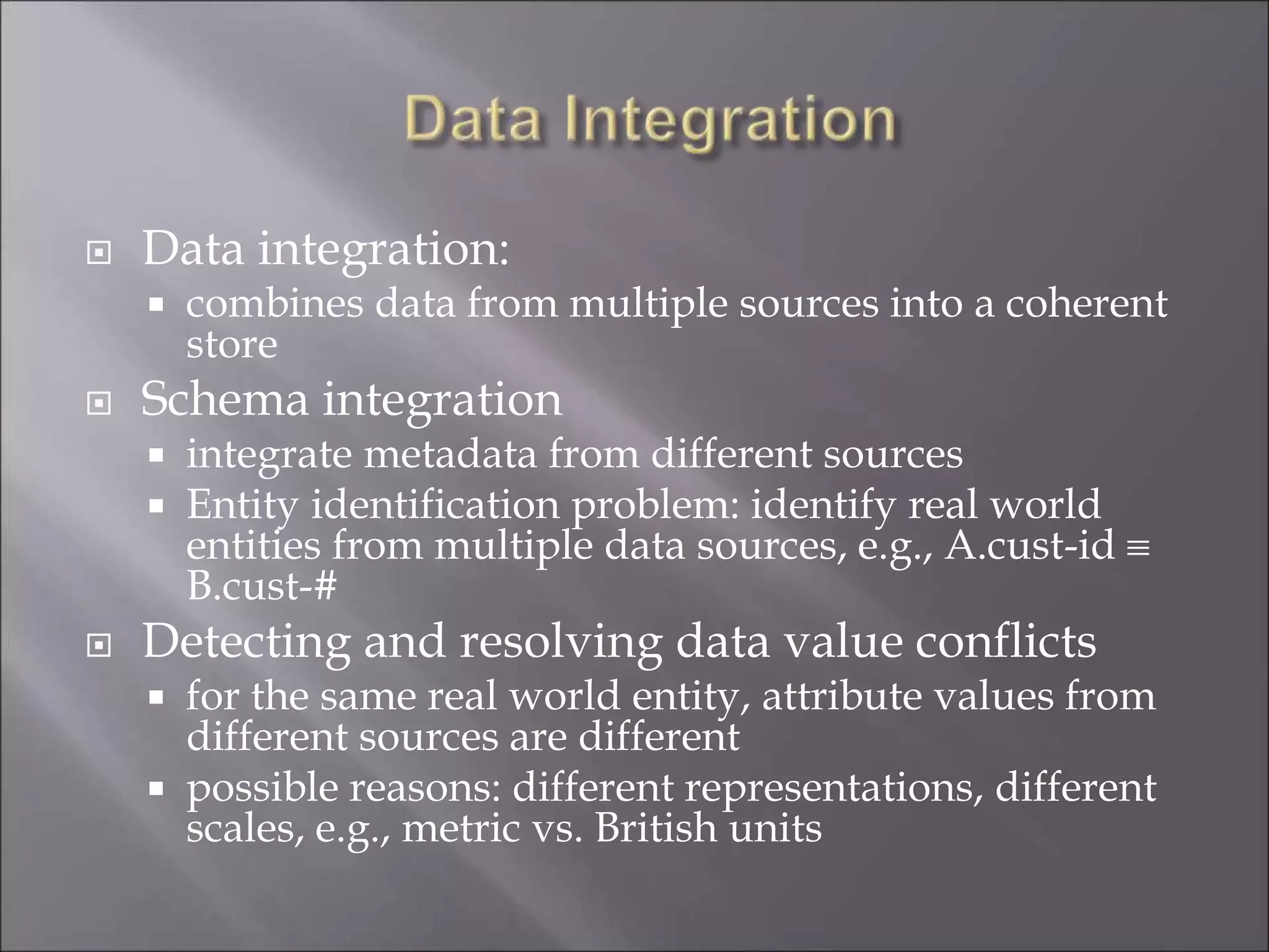
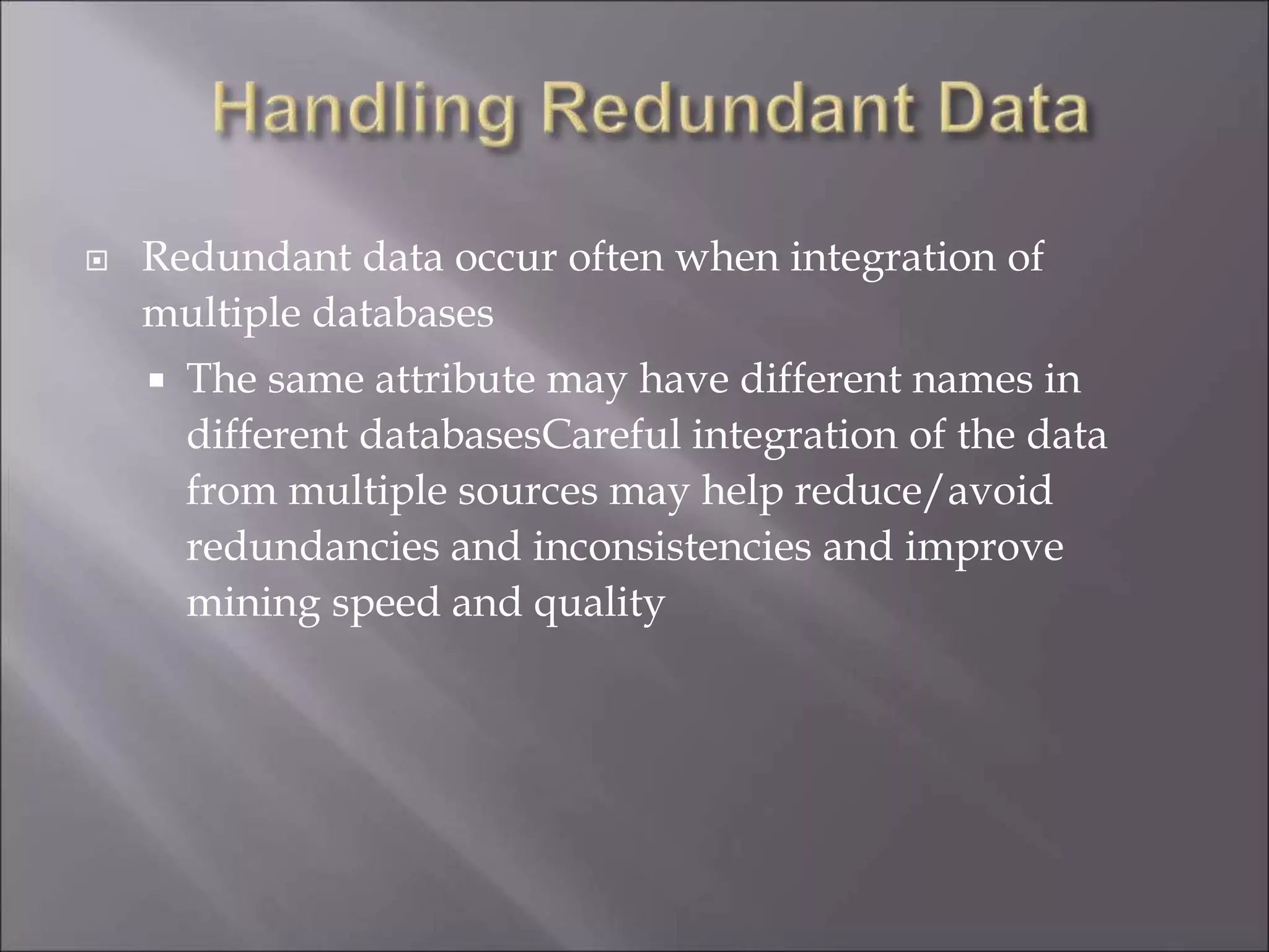
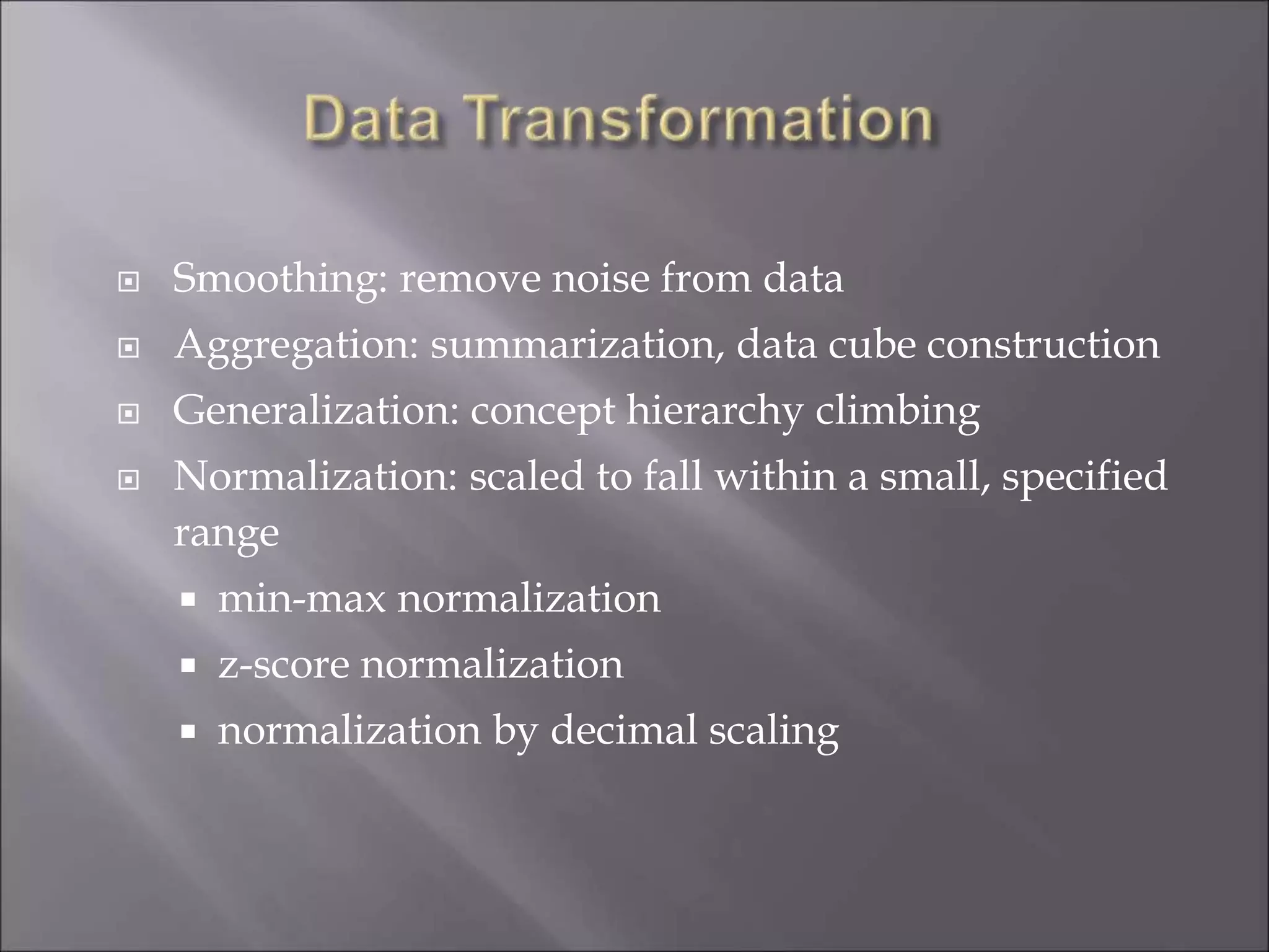
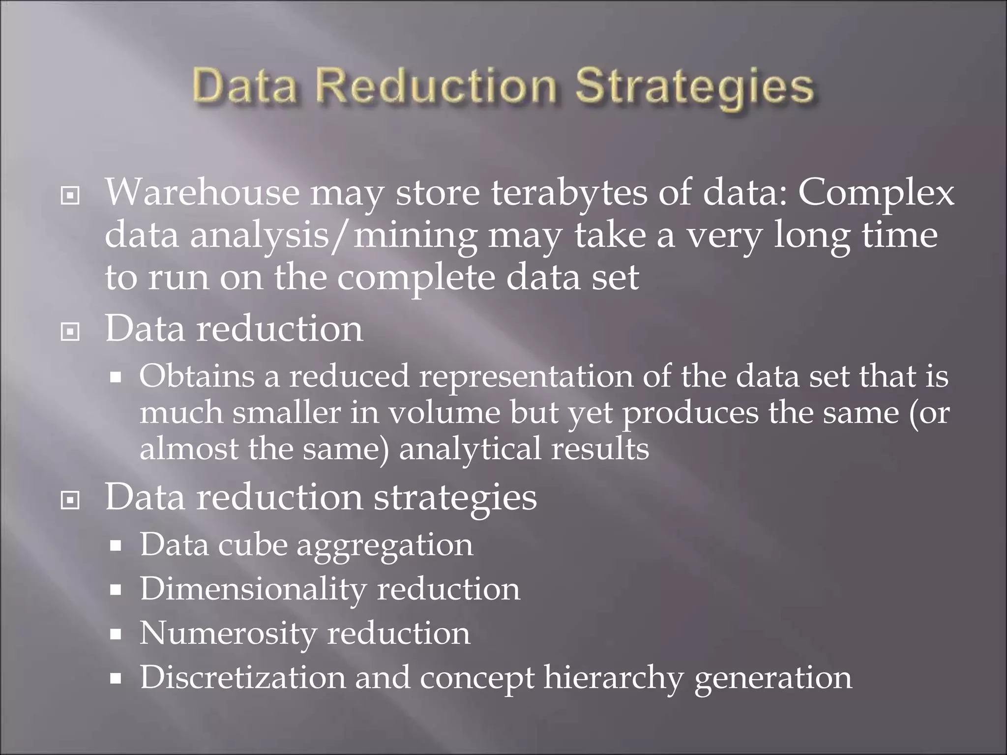
KEMBAR78
Data preprocessing in Data Mining | PPT
 Data in the real world is dirty
 incomplete: lacking attribute values, lacking certain
attributes of interest, or containing only aggregate
data
 noisy: containing errors or outliers
 inconsistent: containing discrepancies in codes or
names
 No quality data, no quality mining results!
 Quality decisions must be based on quality data
 Data warehouse needs consistent integration of
quality data
 Data cleaning
 Fill in missing values, smooth noisy data, identify or remove
outliers, and resolve inconsistencies
 Data integration
 Integration of multiple databases, data cubes, or files
 Data transformation
 Normalization and aggregation
 Data reduction
 Obtains reduced representation in volume but produces the same
or similar analytical results
 Data discretization
 Part of data reduction but with particular importance, especially
for numerical data
 Data cleaning tasks
• Fill in missing values
• Identify outliers and smooth out noisy data
• Correct inconsistent data
• Data is not always available
 E.g., many tuples have no recorded value for several
attributes, such as customer income in sales data
• Missing data may be due to
 equipment malfunction
 inconsistent with other recorded data and thus deleted
 data not entered due to misunderstanding
 certain data may not be considered important at the time of
entry
 not register history or changes of the data
• Missing data may need to be inferred.
 Ignore the tuple: usually done when class label is missing
(assuming the tasks in classification—not effective when the
percentage of missing values per attribute varies considerably)
 Fill in the missing value manually: tedious + infeasible?
 Use a global constant to fill in the missing value: e.g., “unknown”,
a new class?!
 Use the attribute mean to fill in the missing value
 Use the most probable value to fill in the missing value: inference-
based such as Bayesian formula or decision tree
• Noise: random error or variance in a measured variable
• Incorrect attribute values may due to
 faulty data collection instruments
 data entry problems
 data transmission problems
 technology limitation
 inconsistency in naming convention
• Other data problems which requires data cleaning
 duplicate records
 incomplete data
 inconsistent data
 Binning method:
 first sort data and partition into (equi-depth) bins
 then smooth by bin means, smooth by bin median,
smooth by bin boundaries, etc.
 Clustering
 detect and remove outliers
 Combined computer and human inspection
 detect suspicious values and check by human
 Regression
 smooth by fitting the data into regression functions
 Equal-width (distance) partitioning:
 It divides the range into N intervals of equal size: uniform grid
 if A and B are the lowest and highest values of the attribute, the
width of intervals will be: W = (B-A)/N.
 The most straightforward
 But outliers may dominate presentation
 Skewed data is not handled well.
 Equal-depth (frequency) partitioning:
 It divides the range into N intervals, each containing
approximately same number of samples
 Good data scaling
 Managing categorical attributes can be tricky.
* Sorted data for price (in dollars): 4, 8, 9, 15, 21, 21, 24, 25, 26, 28, 29, 34
* Partition into (equi-depth) bins:
- Bin 1: 4, 8, 9, 15
- Bin 2: 21, 21, 24, 25
- Bin 3: 26, 28, 29, 34
* Smoothing by bin means:
- Bin 1: 9, 9, 9, 9
- Bin 2: 23, 23, 23, 23
- Bin 3: 29, 29, 29, 29
* Smoothing by bin boundaries:
- Bin 1: 4, 4, 4, 15
- Bin 2: 21, 21, 25, 25
- Bin 3: 26, 26, 26, 34
 Data integration:
 combines data from multiple sources into a coherent
store
 Schema integration
 integrate metadata from different sources
 Entity identification problem: identify real world
entities from multiple data sources, e.g., A.cust-id 
B.cust-#
 Detecting and resolving data value conflicts
 for the same real world entity, attribute values from
different sources are different
 possible reasons: different representations, different
scales, e.g., metric vs. British units
 Redundant data occur often when integration of
multiple databases
 The same attribute may have different names in
different databasesCareful integration of the data
from multiple sources may help reduce/avoid
redundancies and inconsistencies and improve
mining speed and quality
 Smoothing: remove noise from data
 Aggregation: summarization, data cube construction
 Generalization: concept hierarchy climbing
 Normalization: scaled to fall within a small, specified
range
 min-max normalization
 z-score normalization
 normalization by decimal scaling
 min-max normalization
 z-score normalization
 normalization by decimal scaling
AAA
AA
A
minnewminnewmaxnew
minmax
minv
v _)__(' 



A
A
devstand
meanv
v
_
'


j
v
v
10
' Where j is the smallest integer such that Max(| |)<1'v
 Warehouse may store terabytes of data: Complex
data analysis/mining may take a very long time
to run on the complete data set
 Data reduction
 Obtains a reduced representation of the data set that is
much smaller in volume but yet produces the same (or
almost the same) analytical results
 Data reduction strategies
 Data cube aggregation
 Dimensionality reduction
 Numerosity reduction
 Discretization and concept hierarchy generation
 The lowest level of a data cube
 the aggregated data for an individual entity of interest
 e.g., a customer in a phone calling data warehouse.
 Multiple levels of aggregation in data cubes
 Further reduce the size of data to deal with
 Reference appropriate levels
 Use the smallest representation which is enough to
solve the task
 Feature selection (i.e., attribute subset selection):
 Select a minimum set of features such that the
probability distribution of different classes given the
values for those features is as close as possible to the
original distribution given the values of all features
 reduce # of patterns in the patterns, easier to
understand
Initial attribute set:
{A1, A2, A3, A4, A5, A6}
A4 ?
A1? A6?
Class 1 Class 2 Class 1 Class 2
> Reduced attribute set: {A1, A4, A6}
 Linear regression: Data are modeled to fit a straight
line
 Often uses the least-square method to fit the line
 Multiple regression: allows a response variable Y to be
modeled as a linear function of multidimensional
feature vector
 Log-linear model: approximates discrete
multidimensional probability distributions
 Linear regression: Y =  +  X
 Two parameters ,  and  specify the line and are to
be estimated by using the data at hand.
 using the least squares criterion to the known values
of Y1, Y2, …, X1, X2, ….
 Multiple regression: Y = b0 + b1 X1 + b2 X2.
 Many nonlinear functions can be transformed into the
above.
 Log-linear models:
 The multi-way table of joint probabilities is
approximated by a product of lower-order tables.
 Probability: p(a, b, c, d) = ab acad bcd
 A popular data
reduction technique
 Divide data into
buckets and store
average (sum) for each
bucket
 Can be constructed
optimally in one
dimension using
dynamic programming
 Related to quantization
problems. 0
5
10
15
20
25
30
35
40
10000 30000 50000 70000 90000
 Partition data set into clusters, and one can store
cluster representation only
 Can be very effective if data is clustered but not if data
is “smeared”
 Can have hierarchical clustering and be stored in
multi-dimensional index tree structures
 There are many choices of clustering definitions and
clustering algorithms, further detailed in Chapter 8
 Allow a mining algorithm to run in complexity that is
potentially sub-linear to the size of the data
 Choose a representative subset of the data
 Simple random sampling may have very poor
performance in the presence of skew
 Develop adaptive sampling methods
 Stratified sampling:
 Approximate the percentage of each class (or
subpopulation of interest) in the overall database
 Used in conjunction with skewed data
Sampling
Raw Data
 Three types of attributes:
 Nominal — values from an unordered set
 Ordinal — values from an ordered set
 Continuous — real numbers
 Discretization:
divide the range of a continuous attribute into
intervals
 Some classification algorithms only accept
categorical attributes.
 Reduce data size by discretization
 Prepare for further analysis
 Discretization
 reduce the number of values for a given continuous
attribute by dividing the range of the attribute into
intervals. Interval labels can then be used to replace
actual data values.
 Concept hierarchies
 reduce the data by collecting and replacing low
level concepts (such as numeric values for the
attribute age) by higher level concepts (such as
young, middle-aged, or senior).

Data preprocessing in Data Mining

  • 2.
     Data inthe real world is dirty  incomplete: lacking attribute values, lacking certain attributes of interest, or containing only aggregate data  noisy: containing errors or outliers  inconsistent: containing discrepancies in codes or names  No quality data, no quality mining results!  Quality decisions must be based on quality data  Data warehouse needs consistent integration of quality data
  • 3.
     Data cleaning Fill in missing values, smooth noisy data, identify or remove outliers, and resolve inconsistencies  Data integration  Integration of multiple databases, data cubes, or files  Data transformation  Normalization and aggregation  Data reduction  Obtains reduced representation in volume but produces the same or similar analytical results  Data discretization  Part of data reduction but with particular importance, especially for numerical data
  • 5.
     Data cleaningtasks • Fill in missing values • Identify outliers and smooth out noisy data • Correct inconsistent data
  • 6.
    • Data isnot always available  E.g., many tuples have no recorded value for several attributes, such as customer income in sales data • Missing data may be due to  equipment malfunction  inconsistent with other recorded data and thus deleted  data not entered due to misunderstanding  certain data may not be considered important at the time of entry  not register history or changes of the data • Missing data may need to be inferred.
  • 7.
     Ignore thetuple: usually done when class label is missing (assuming the tasks in classification—not effective when the percentage of missing values per attribute varies considerably)  Fill in the missing value manually: tedious + infeasible?  Use a global constant to fill in the missing value: e.g., “unknown”, a new class?!  Use the attribute mean to fill in the missing value  Use the most probable value to fill in the missing value: inference- based such as Bayesian formula or decision tree
  • 8.
    • Noise: randomerror or variance in a measured variable • Incorrect attribute values may due to  faulty data collection instruments  data entry problems  data transmission problems  technology limitation  inconsistency in naming convention • Other data problems which requires data cleaning  duplicate records  incomplete data  inconsistent data
  • 9.
     Binning method: first sort data and partition into (equi-depth) bins  then smooth by bin means, smooth by bin median, smooth by bin boundaries, etc.  Clustering  detect and remove outliers  Combined computer and human inspection  detect suspicious values and check by human  Regression  smooth by fitting the data into regression functions
  • 10.
     Equal-width (distance)partitioning:  It divides the range into N intervals of equal size: uniform grid  if A and B are the lowest and highest values of the attribute, the width of intervals will be: W = (B-A)/N.  The most straightforward  But outliers may dominate presentation  Skewed data is not handled well.  Equal-depth (frequency) partitioning:  It divides the range into N intervals, each containing approximately same number of samples  Good data scaling  Managing categorical attributes can be tricky.
  • 11.
    * Sorted datafor price (in dollars): 4, 8, 9, 15, 21, 21, 24, 25, 26, 28, 29, 34 * Partition into (equi-depth) bins: - Bin 1: 4, 8, 9, 15 - Bin 2: 21, 21, 24, 25 - Bin 3: 26, 28, 29, 34 * Smoothing by bin means: - Bin 1: 9, 9, 9, 9 - Bin 2: 23, 23, 23, 23 - Bin 3: 29, 29, 29, 29 * Smoothing by bin boundaries: - Bin 1: 4, 4, 4, 15 - Bin 2: 21, 21, 25, 25 - Bin 3: 26, 26, 26, 34
  • 12.
     Data integration: combines data from multiple sources into a coherent store  Schema integration  integrate metadata from different sources  Entity identification problem: identify real world entities from multiple data sources, e.g., A.cust-id  B.cust-#  Detecting and resolving data value conflicts  for the same real world entity, attribute values from different sources are different  possible reasons: different representations, different scales, e.g., metric vs. British units
  • 13.
     Redundant dataoccur often when integration of multiple databases  The same attribute may have different names in different databasesCareful integration of the data from multiple sources may help reduce/avoid redundancies and inconsistencies and improve mining speed and quality
  • 14.
     Smoothing: removenoise from data  Aggregation: summarization, data cube construction  Generalization: concept hierarchy climbing  Normalization: scaled to fall within a small, specified range  min-max normalization  z-score normalization  normalization by decimal scaling
  • 15.
     min-max normalization z-score normalization  normalization by decimal scaling AAA AA A minnewminnewmaxnew minmax minv v _)__('     A A devstand meanv v _ '   j v v 10 ' Where j is the smallest integer such that Max(| |)<1'v
  • 16.
     Warehouse maystore terabytes of data: Complex data analysis/mining may take a very long time to run on the complete data set  Data reduction  Obtains a reduced representation of the data set that is much smaller in volume but yet produces the same (or almost the same) analytical results  Data reduction strategies  Data cube aggregation  Dimensionality reduction  Numerosity reduction  Discretization and concept hierarchy generation
  • 17.
     The lowestlevel of a data cube  the aggregated data for an individual entity of interest  e.g., a customer in a phone calling data warehouse.  Multiple levels of aggregation in data cubes  Further reduce the size of data to deal with  Reference appropriate levels  Use the smallest representation which is enough to solve the task
  • 18.
     Feature selection(i.e., attribute subset selection):  Select a minimum set of features such that the probability distribution of different classes given the values for those features is as close as possible to the original distribution given the values of all features  reduce # of patterns in the patterns, easier to understand
  • 19.
    Initial attribute set: {A1,A2, A3, A4, A5, A6} A4 ? A1? A6? Class 1 Class 2 Class 1 Class 2 > Reduced attribute set: {A1, A4, A6}
  • 20.
     Linear regression:Data are modeled to fit a straight line  Often uses the least-square method to fit the line  Multiple regression: allows a response variable Y to be modeled as a linear function of multidimensional feature vector  Log-linear model: approximates discrete multidimensional probability distributions
  • 21.
     Linear regression:Y =  +  X  Two parameters ,  and  specify the line and are to be estimated by using the data at hand.  using the least squares criterion to the known values of Y1, Y2, …, X1, X2, ….  Multiple regression: Y = b0 + b1 X1 + b2 X2.  Many nonlinear functions can be transformed into the above.  Log-linear models:  The multi-way table of joint probabilities is approximated by a product of lower-order tables.  Probability: p(a, b, c, d) = ab acad bcd
  • 22.
     A populardata reduction technique  Divide data into buckets and store average (sum) for each bucket  Can be constructed optimally in one dimension using dynamic programming  Related to quantization problems. 0 5 10 15 20 25 30 35 40 10000 30000 50000 70000 90000
  • 23.
     Partition dataset into clusters, and one can store cluster representation only  Can be very effective if data is clustered but not if data is “smeared”  Can have hierarchical clustering and be stored in multi-dimensional index tree structures  There are many choices of clustering definitions and clustering algorithms, further detailed in Chapter 8
  • 24.
     Allow amining algorithm to run in complexity that is potentially sub-linear to the size of the data  Choose a representative subset of the data  Simple random sampling may have very poor performance in the presence of skew  Develop adaptive sampling methods  Stratified sampling:  Approximate the percentage of each class (or subpopulation of interest) in the overall database  Used in conjunction with skewed data
  • 25.
  • 26.
     Three typesof attributes:  Nominal — values from an unordered set  Ordinal — values from an ordered set  Continuous — real numbers  Discretization: divide the range of a continuous attribute into intervals  Some classification algorithms only accept categorical attributes.  Reduce data size by discretization  Prepare for further analysis
  • 27.
     Discretization  reducethe number of values for a given continuous attribute by dividing the range of the attribute into intervals. Interval labels can then be used to replace actual data values.  Concept hierarchies  reduce the data by collecting and replacing low level concepts (such as numeric values for the attribute age) by higher level concepts (such as young, middle-aged, or senior).