The document discusses design of experiments (DOE) and provides details about:
1) DOE is a process optimization technique that relies on planned experimentation and statistical analysis to study multiple factors and their interactions.
2) Traditional experimentation methods study one factor at a time and ignore interactions, while DOE allows studying multiple factors and interactions using fewer experiments.
3) Steps for DOE include defining objectives, factors, responses, levels, and designing the experiment using full or fractional factorial designs such as orthogonal arrays.
Presentation by the Society of Statistical Quality Control Engineers on the Design of Experiments (DOE) as a critical process optimization technique.
DOE defined as a systematic approach to experimentation, maximizing data from planned experiments for process optimization.
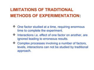
Traditional experimentation methods are inefficient, studying one factor at a time and ignoring interactions, leading to lengthy experiments and potential errors.
DOE optimizes processes with fewer trials, considers interactions, utilizes ANOVA for data analysis, and employs Orthogonal Arrays for efficient designs.
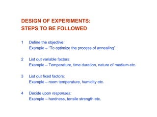
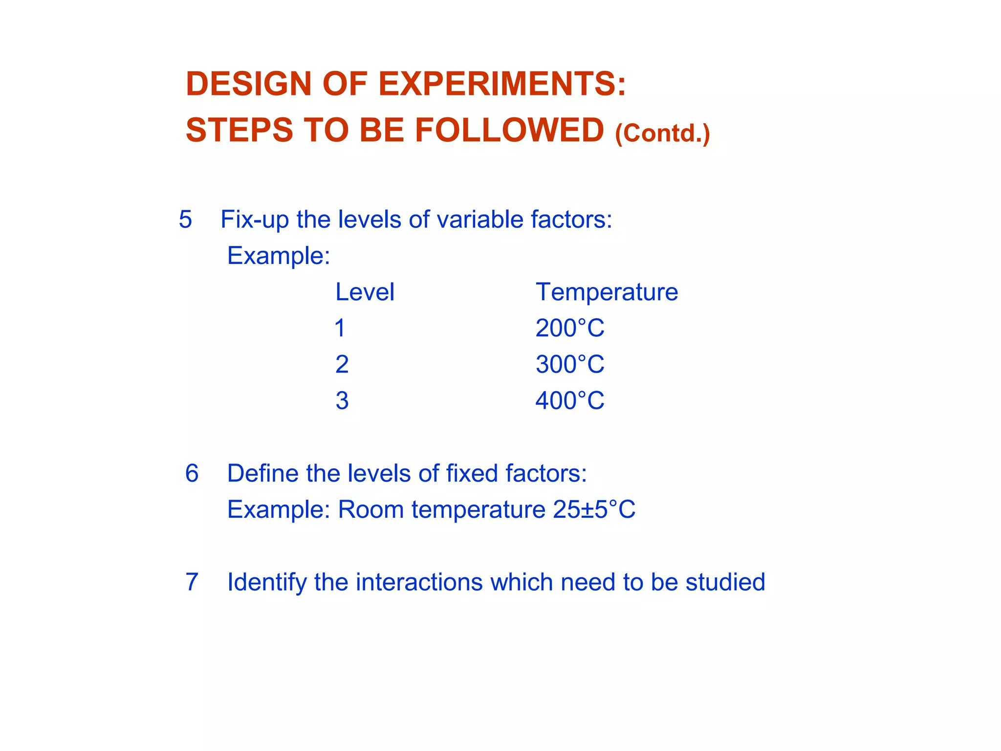
Initial steps in DOE include defining objectives, identifying variable and fixed factors, and outlining response variables for the experiment.
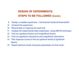
Continued steps in DOE involve fixing factor levels, identifying necessary interactions, and preparing experimental designs.
Final steps involve conducting the experiments, recording data, analyzing results through ANOVA, identifying significant factors, and reporting optimum levels.
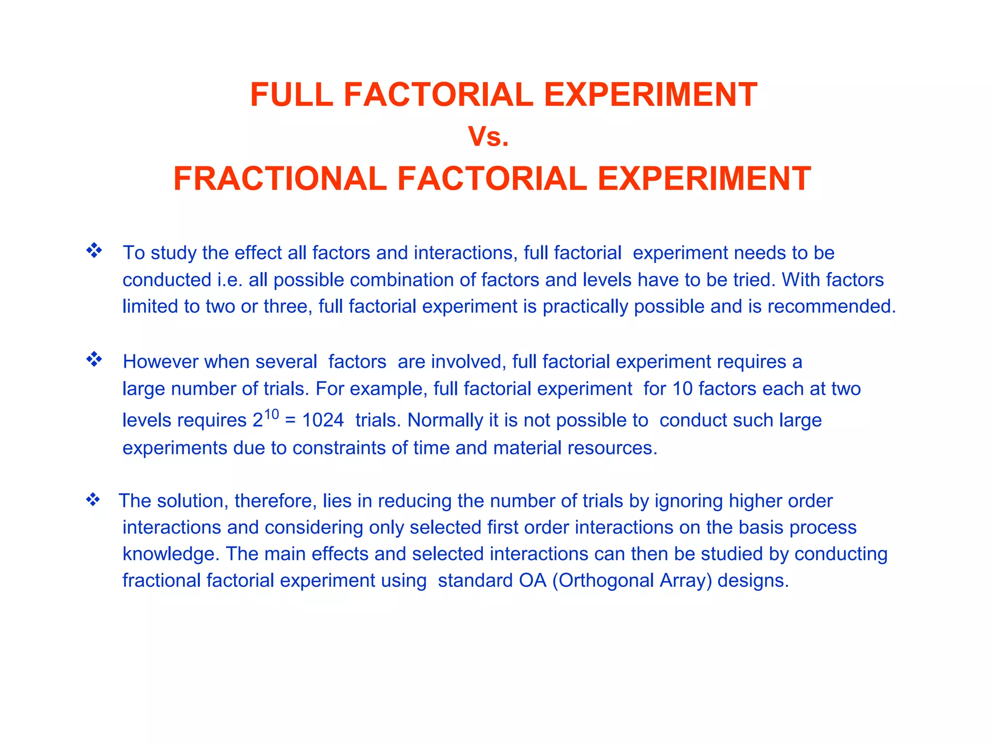
Full factorial experiments provide comprehensive data but may require impractical trials, whereas fractional factorial designs reduce trial numbers by focusing on significant interactions.
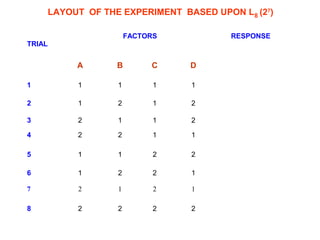
Published orthogonal arrays allow for efficient experimental designs based on factors and interactions, categorized into various levels.
Overview of practical examples to illustrate the application of DOE principles.
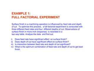
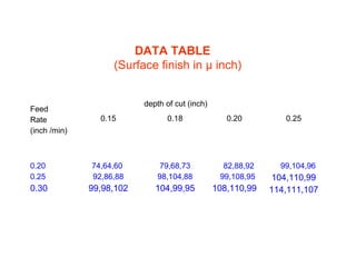
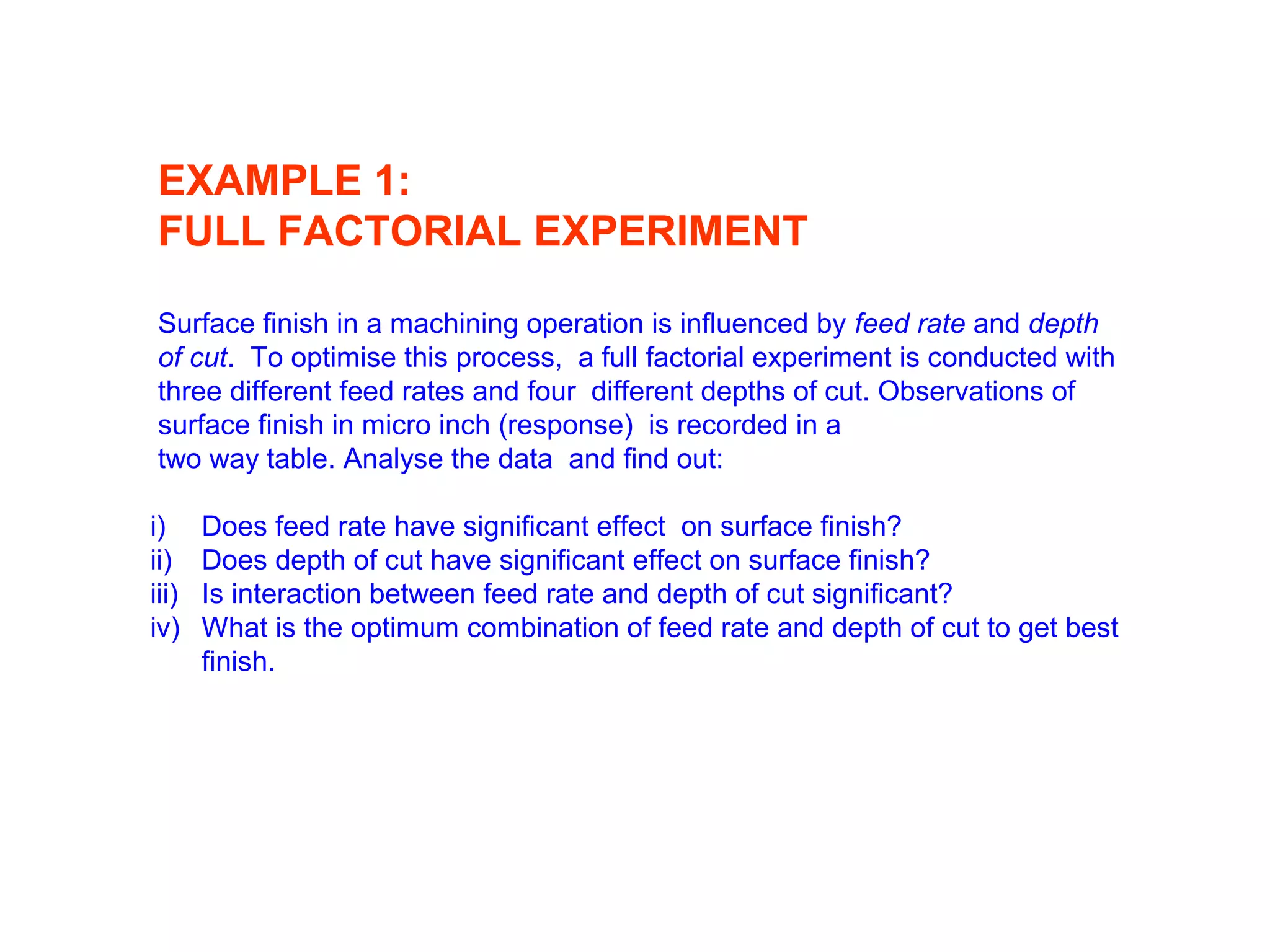
Case study on surface finish affected by feed rate and depth of cut using a full factorial experiment.
Data table recording surface finish related to different feed rates and depths of cut from the factorial experiment for further analysis.
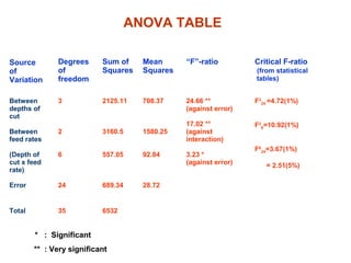
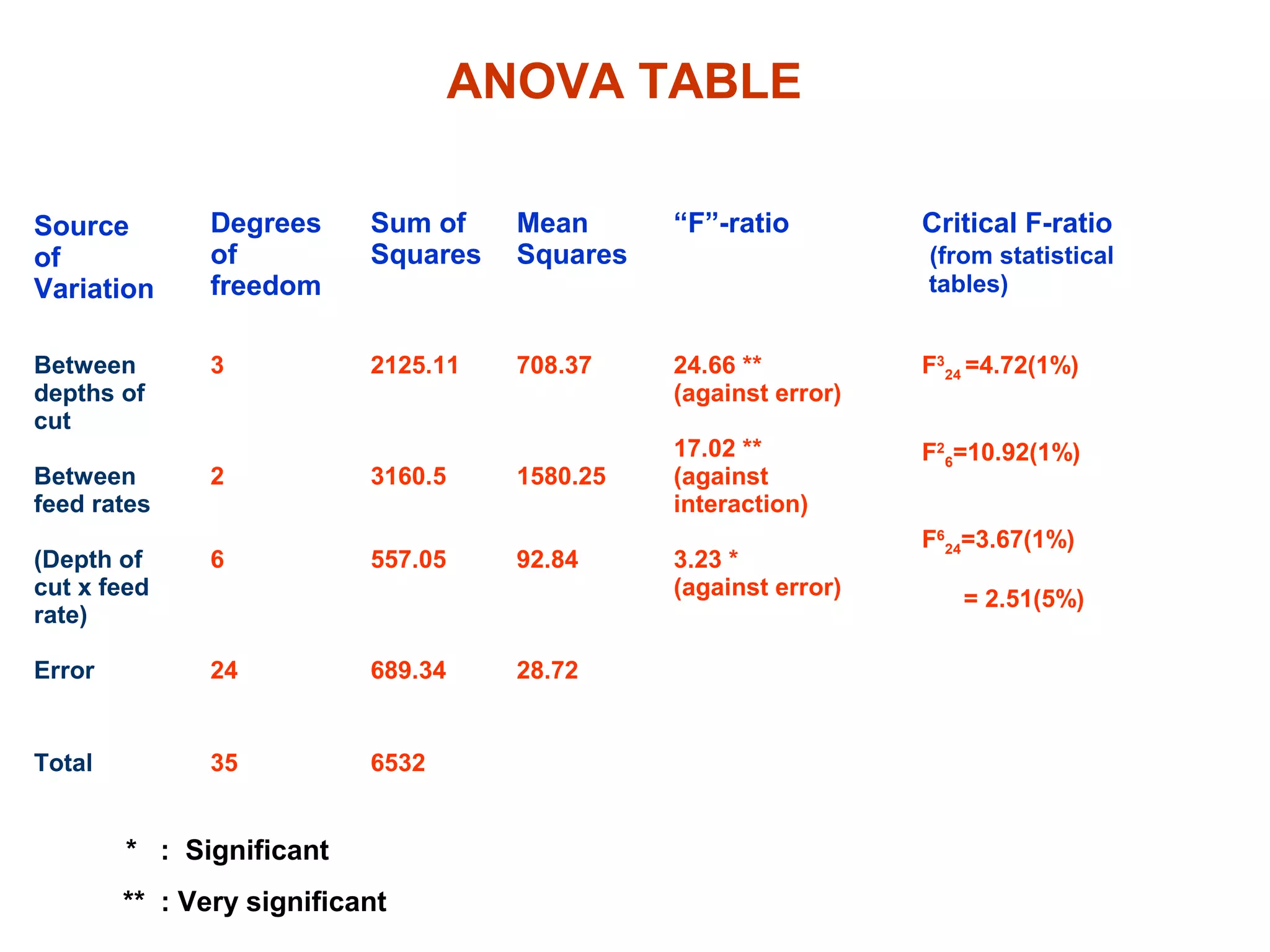
ANOVA results detailing variations due to depth of cut and feed rates, including significance levels of factors and their interactions.
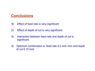
Key findings indicate significant effects of both feed rate and depth of cut on surface finish, with optimal parameters identified.
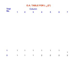
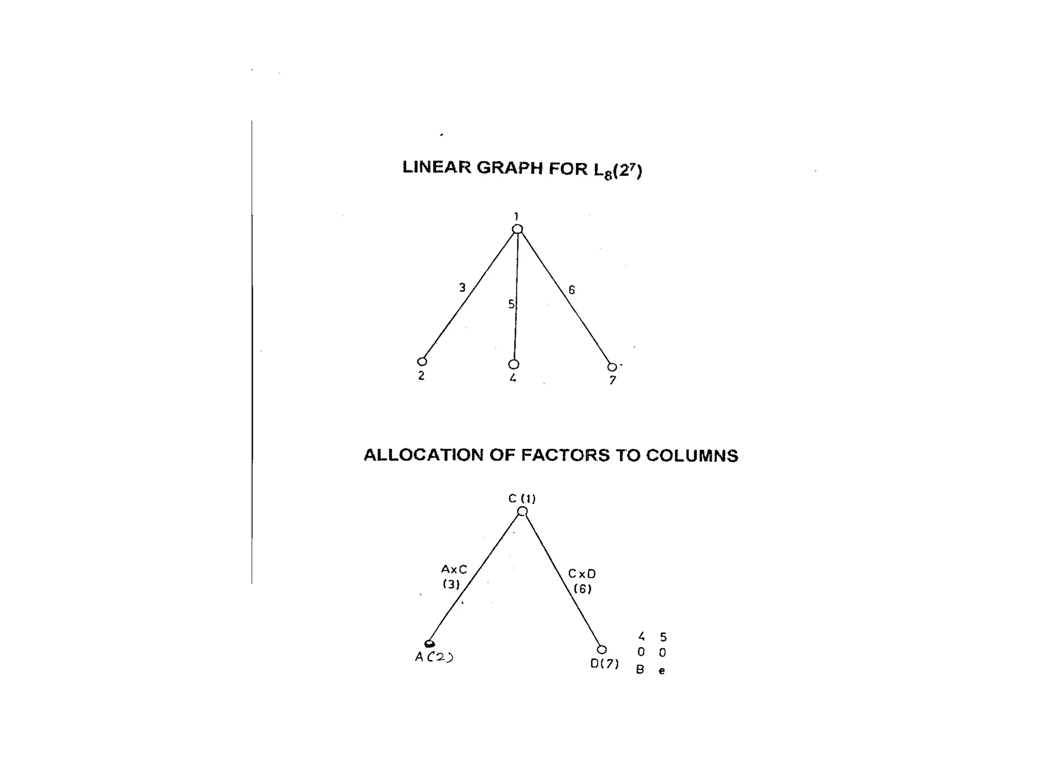
Design practice involves four factors with selected interactions to illustrate the application of orthogonal arrays in DOE.
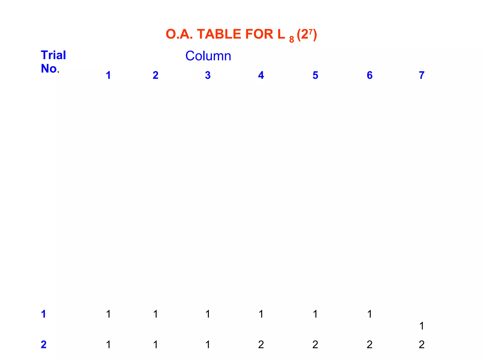
Formation of an orthogonal array table for systematic testing of factors in the designed experiment.
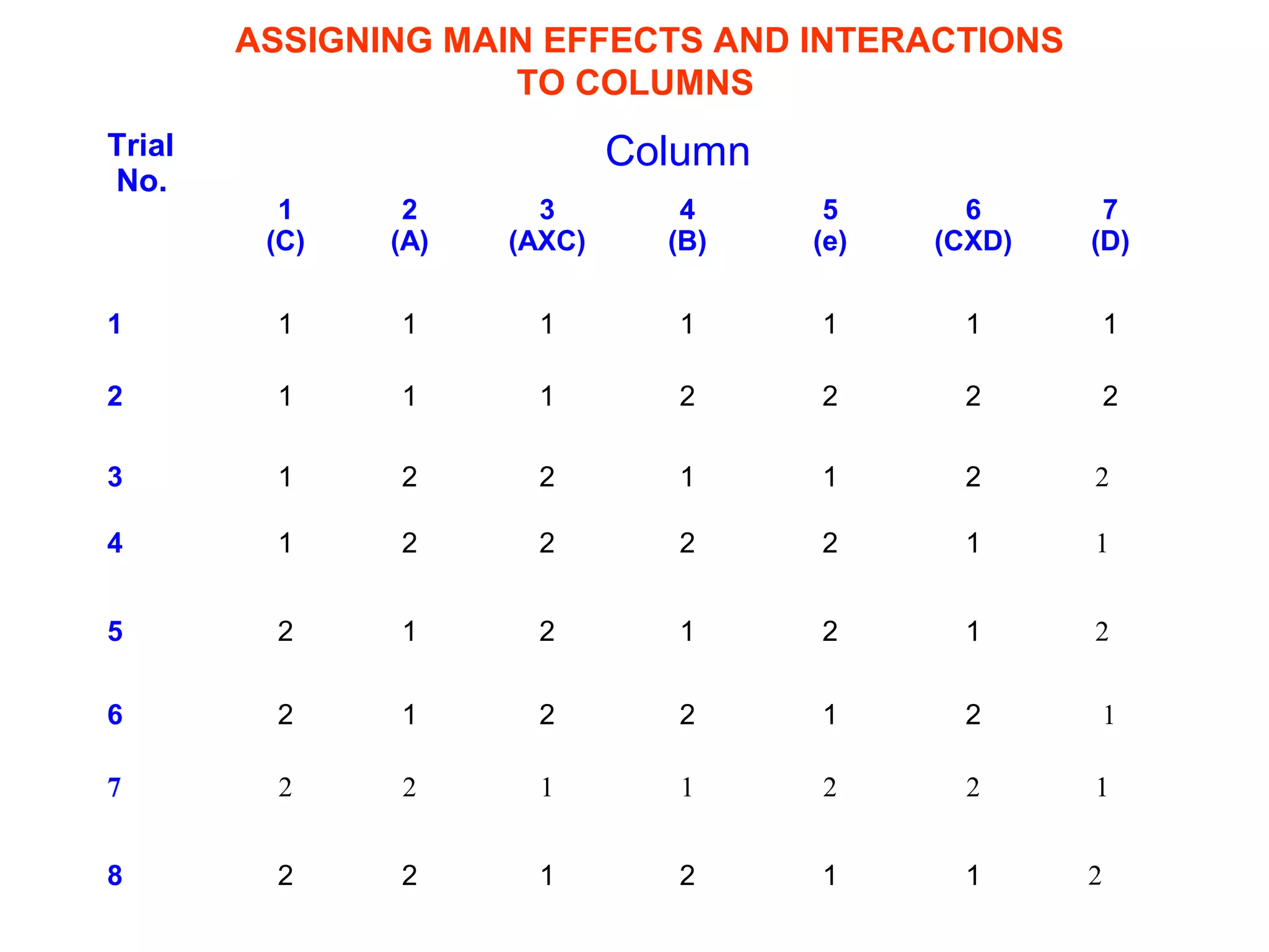
Methodology for assigning main effects and interactions to experimental design columns in orthogonal array.
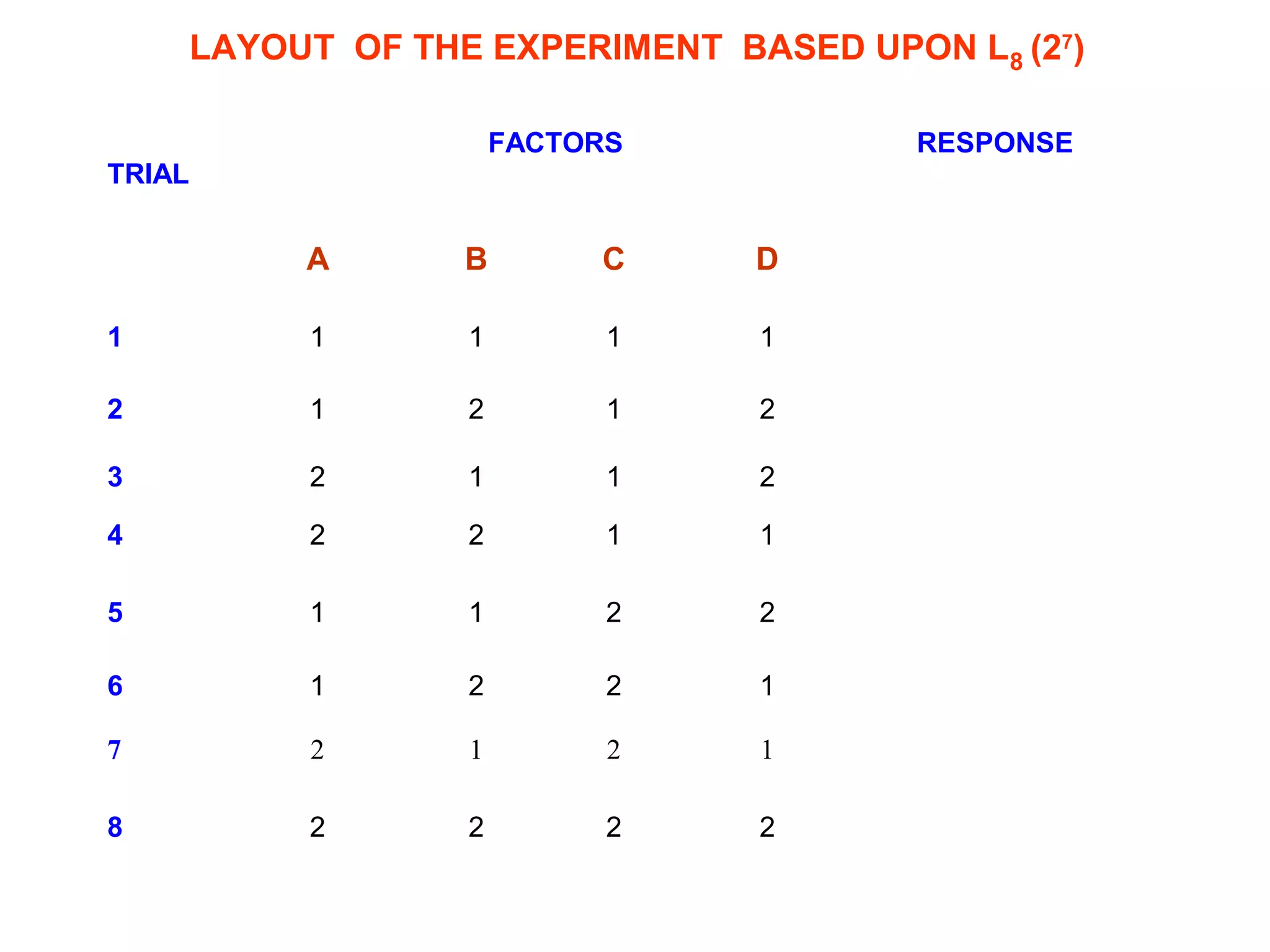
Final layout of the experimental design detailing factors and response variables for conducting the trial.
What is DOE
DOEis a process optimization
technique that relies on planned
experimentation and statistical
analysis of results
3.
LIMITATIONS OF TRADITIONAL
METHODSOF EXPERIMENTATION:
One factor studied at a time, requiring enormous
time to complete the experiment.
Interactions i.e. effect of one factor on another, are
ignored leading to erroneous results.
Complex processes involving a number of factors,
levels, interactions can not be studied by traditional
approach.
4.
DOE ADVANTAGES:
Optimizesprocess parameters with minimum number
of trials, thus saving time and resources on
experimentation.
Interactions (effect of one factor on another) also taken
into consideration.
Results analysed using ANOVA technique for
objective judgement.
Orthogonal Arrays (OA) technique used for finding
efficient designs of experiments.
5.
DESIGN OF EXPERIMENTS:
STEPSTO BE FOLLOWED
1 Define the objective:
Example – “To optimize the process of annealing”
2 List out variable factors:
Example – Temperature, time duration, nature of medium etc.
3 List out fixed factors:
Example – room temperature, humidity etc.
4 Decide upon responses:
Example – hardness, tensile strength etc.
6.
DESIGN OF EXPERIMENTS:
STEPSTO BE FOLLOWED (Contd.)
5 Fix-up the levels of variable factors:
Example:
Level Temperature
1 200°C
2 300°C
3 400°C
6 Define the levels of fixed factors:
Example: Room temperature 25±5°C
7 Identify the interactions which need to be studied
7.
DESIGN OF EXPERIMENTS:
STEPSTO BE FOLLOWED (Contd.)
8 Design a suitable experiment – full factorial/ fractional factorial/OA
9 Conduct the experiment
10 Record data on response for each trial
11 Analyse the experimental data (responses) using ANOVA technique
12 Find out significant factors and insignificant factors
13 Find out significant interactions and insignificant interactions
14 Plot response curves to find out optimum levels of significant
factors.
15 Report optimum levels of process parameters as final result
8.
FULL FACTORIAL EXPERIMENT
Vs.
FRACTIONALFACTORIAL EXPERIMENT
To study the effect all factors and interactions, full factorial experiment needs to be
conducted i.e. all possible combination of factors and levels have to be tried. With factors
limited to two or three, full factorial experiment is practically possible and is recommended.
However when several factors are involved, full factorial experiment requires a
large number of trials. For example, full factorial experiment for 10 factors each at two
levels requires 210
= 1024 trials. Normally it is not possible to conduct such large
experiments due to constraints of time and material resources.
The solution, therefore, lies in reducing the number of trials by ignoring higher order
interactions and considering only selected first order interactions on the basis process
knowledge. The main effects and selected interactions can then be studied by conducting
fractional factorial experiment using standard OA (Orthogonal Array) designs.
9.
ABOUT ORTHOGONAL ARRAYDESIGNS
Published orthogonal array designs are available for various experimental sizes
which are in powers of 2,3,4 etc. Depending on the number of factors, levels and
number of interactions to be estimated, a suitable design can be arrived at using
these tables.
Some standard Orthogonal tables are:
2 level series : L8 (27
), L16 (215
), L32 (231
)
3 level series : L9 (34
), L 27 (313
)….
Mixed series : L18 (21
x 37
),
L50 (21
x 5 11
) etc
Thus in L16 (215
), 16 represents the number of experimental trials, 2 the number of
levels at which each factor is examined and 15 the number of columns in the
design.
The allocation of factors and interactions to columns is done with the aid of Linear
Graphs.
EXAMPLE 1:
FULL FACTORIALEXPERIMENT
Surface finish in a machining operation is influenced by feed rate and depth
of cut. To optimise this process, a full factorial experiment is conducted with
three different feed rates and four different depths of cut. Observations of
surface finish in micro inch (response) is recorded in a
two way table. Analyse the data and find out:
i) Does feed rate have significant effect on surface finish?
ii) Does depth of cut have significant effect on surface finish?
iii) Is interaction between feed rate and depth of cut significant?
iv) What is the optimum combination of feed rate and depth of cut to get best
finish.
Source
of
Variation
Degrees
of
freedom
Sum of
Squares
Mean
Squares
“F”-ratio CriticalF-ratio
(from statistical
tables)
Between
depths of
cut
Between
feed rates
(Depth of
cut x feed
rate)
Error
3
2
6
24
2125.11
3160.5
557.05
689.34
708.37
1580.25
92.84
28.72
24.66 **
(against error)
17.02 **
(against
interaction)
3.23 *
(against error)
F3
24 =4.72(1%)
F2
6=10.92(1%)
F6
24=3.67(1%)
= 2.51(5%)
Total 35 6532
ANOVA TABLE
* : Significant
** : Very significant
14.
Conclusions
1) Effect offeed rate is very significant
2) Effect of depth of cut is very significant
3) Interaction between feed rate and depth of cut is
significant.
4) Optimum combination is: feed rate 0.2 inch /min and depth
of cut 0.15 inch
15.
EXAMPLE 2:
DESIGNING EXPERIMENTUSING ORTHOGONAL ARRAYS
No. of factors = 4 (A, B, C, D)
1st Order interactions = AxB, AxC, AxD, BxC, BxD, CxD
2nd Order interactions = AxBxC, BxCxD, CxDxA, DxAxB
3rd Order interaction = AxBxCxD
In practice, only few first order interactions are of interest. Rest of the
interactions can be neglected. In this case , it is given that only two interactions
AxC and CxD are to be considered.