

![Directed Diffusion
Naming
Task descriptions are named by a list of attribute value pairs that
describe a task
eg:
type=wheeled vehicle // detect vehicle location
interval=20ms // send events every 20 ms
duration=10s // for the next 10s
rect=[-100,100,200,400]// from sensors within rectangle
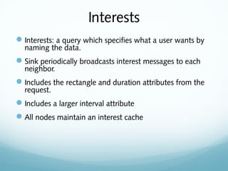
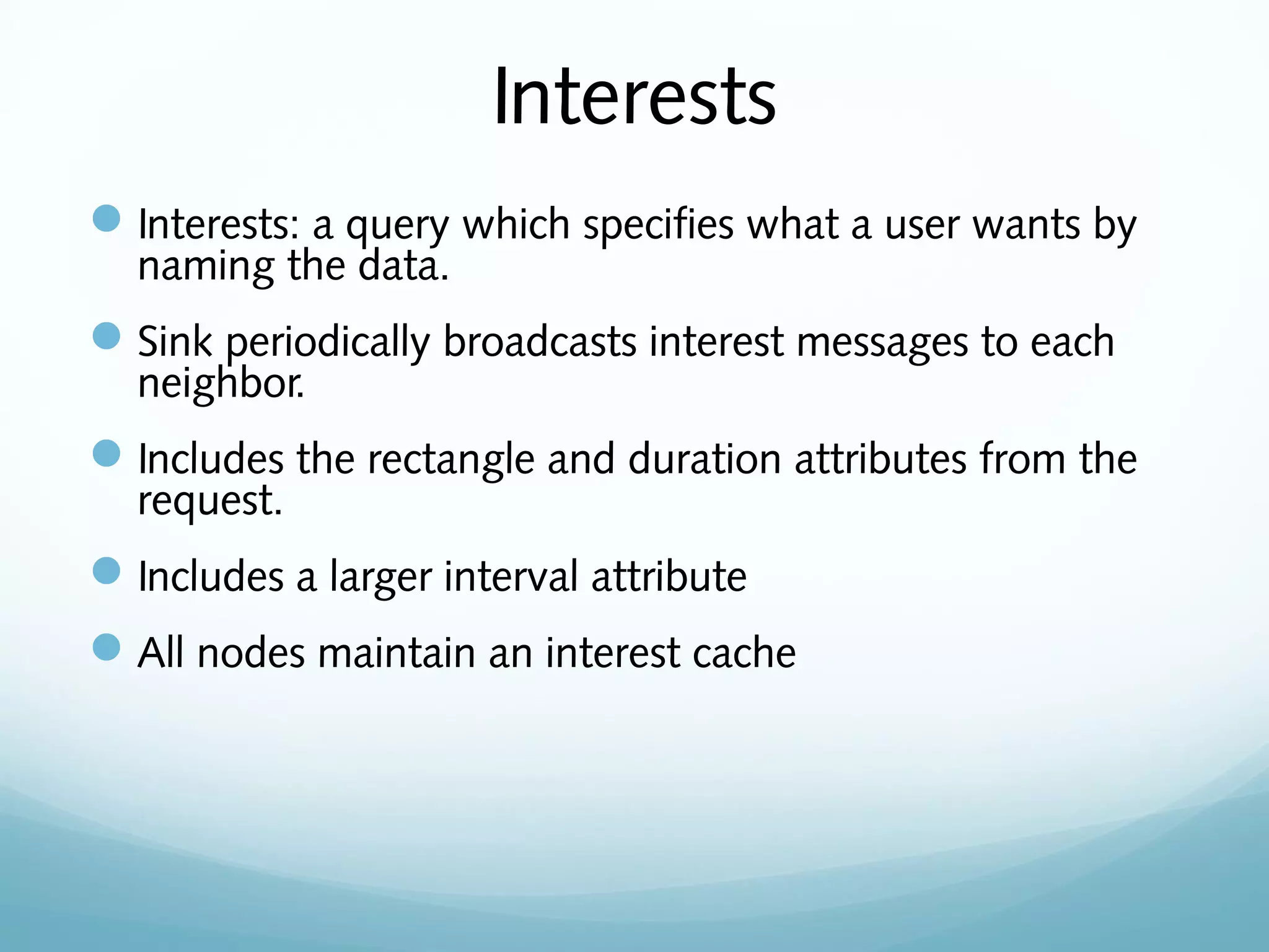
Interests and Gradients
Interest is usually injected to the network from sink
For each active task, sink periodically broadcasts an interest
message to each of its neighbors
Initial interest contains the specified rect and duration attributes
but larger interval attribute
Interests tries to determine if there are any sensor nodes that
detect the wheeled vehicle(exploratory).](https://image.slidesharecdn.com/directeddiffusionforwirelesssensornetworking-130704095551-phpapp02/85/Directed-diffusion-for-wireless-sensor-networking-11-320.jpg)


![Directed Diffusion
Naming
Task descriptions are named by a list of attribute value pairs that
describe a task
eg:
type=wheeled vehicle // detect vehicle location
interval=20ms // send events every 20 ms
duration=10s // for the next 10s
rect=[-100,100,200,400]// from sensors within rectangle
Interests and Gradients
Interest is usually injected to the network from sink
For each active task, sink periodically broadcasts an interest
message to each of its neighbors
Initial interest contains the specified rect and duration attributes
but larger interval attribute
Interests tries to determine if there are any sensor nodes that
detect the wheeled vehicle(exploratory).](https://image.slidesharecdn.com/directeddiffusionforwirelesssensornetworking-130704095551-phpapp02/75/Directed-diffusion-for-wireless-sensor-networking-11-2048.jpg)


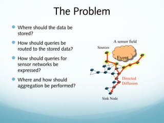
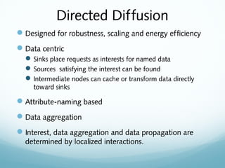
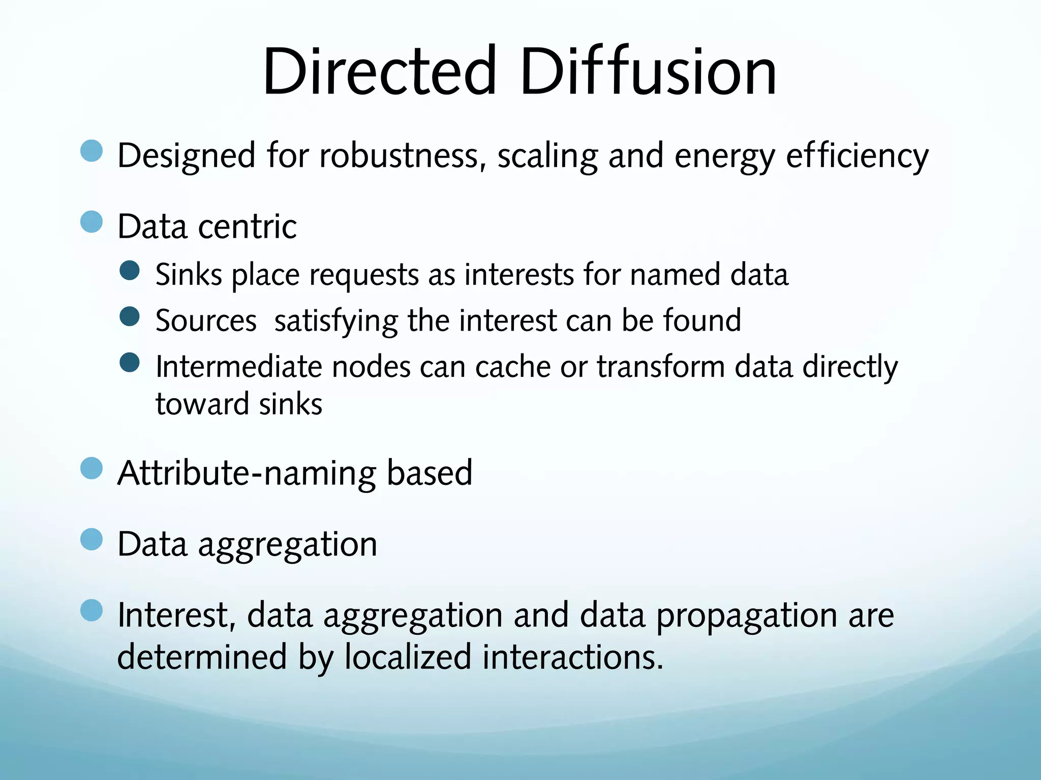
This document summarizes the key ideas of the "Directed Diffusion for Wireless Sensor Networking" paper. It introduces directed diffusion as a data-centric paradigm for wireless sensor networks that is designed for robustness, scalability, and energy efficiency. The core concepts of directed diffusion are interests, data, gradients, and reinforcement, which work together to efficiently route queries to sensor data in the network. Through localized interactions and data aggregation, directed diffusion is shown to significantly reduce energy consumption compared to flooding-based approaches in wireless sensor networks.
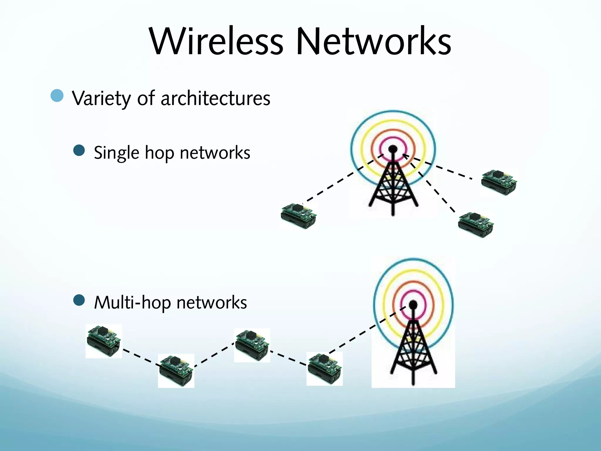
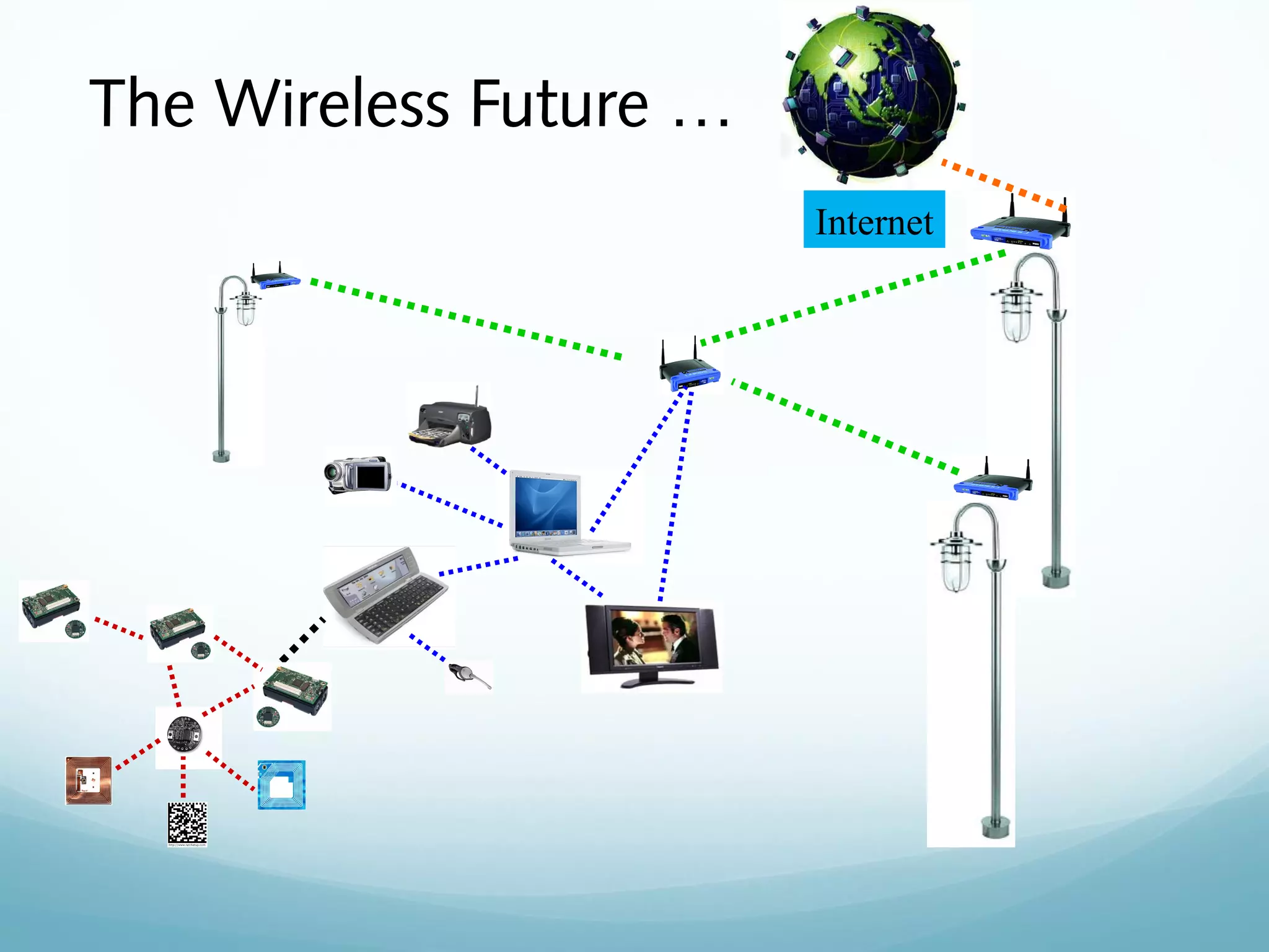
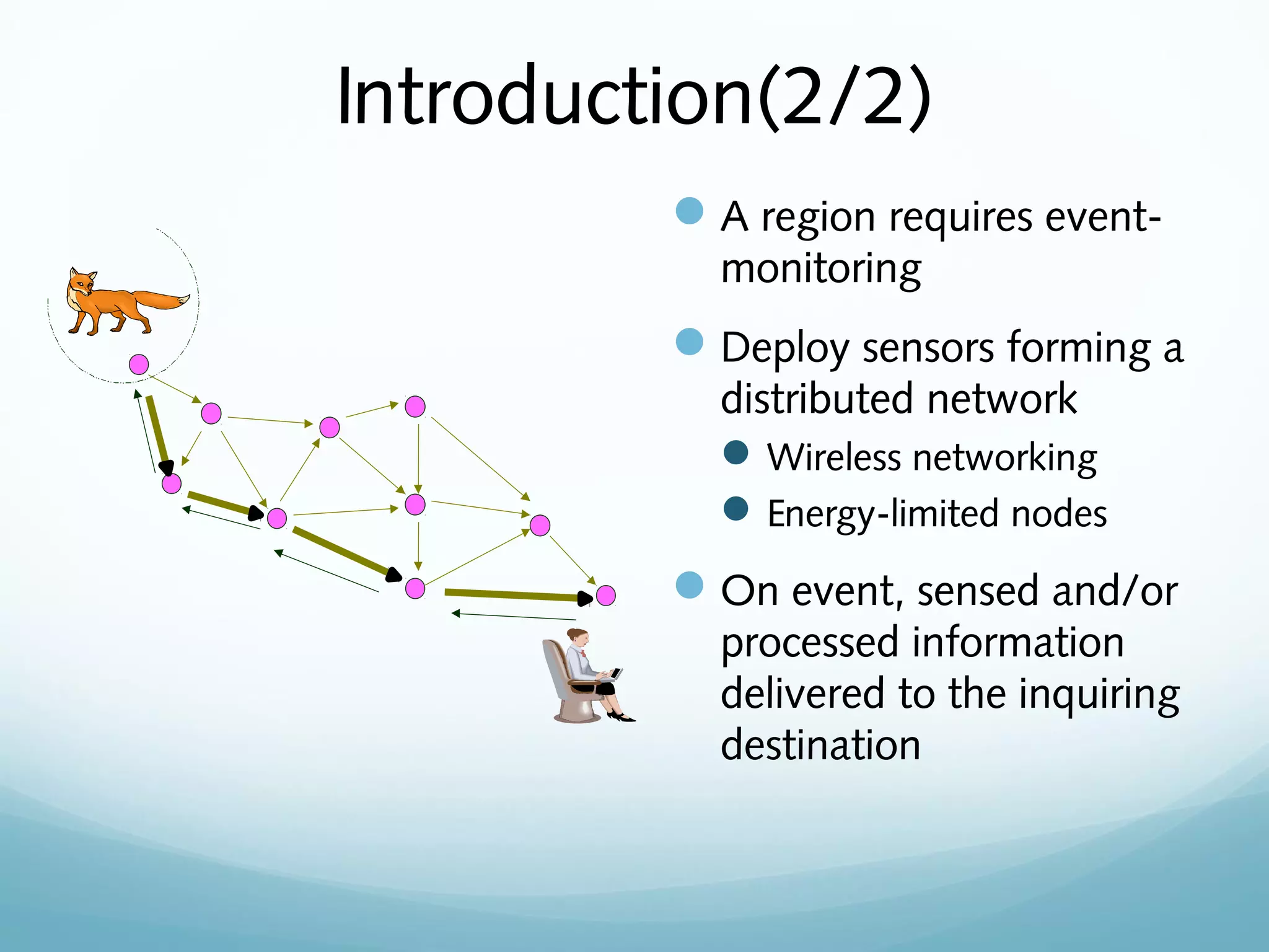
Introduction to wireless sensor networks, discussing architectures, properties, and deployment.
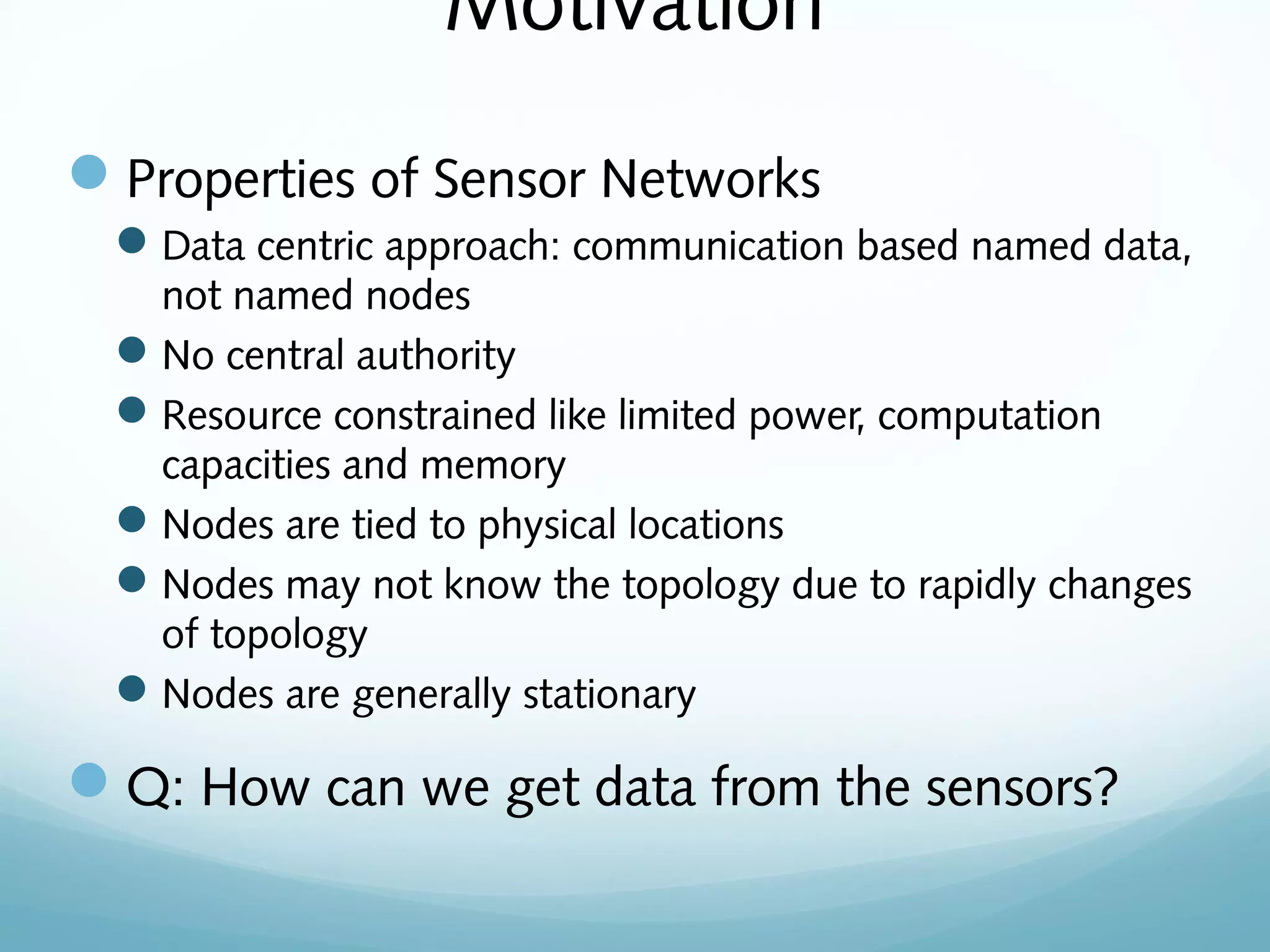
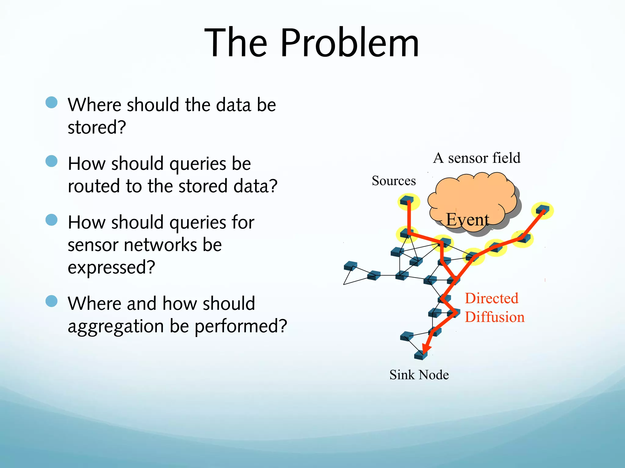
Key problems in sensor networks, introducing directed diffusion as a solution focusing on data-centric approaches.
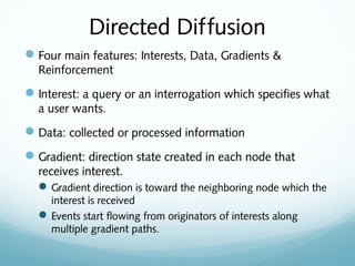
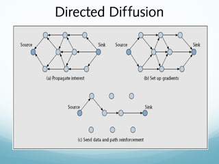
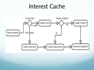
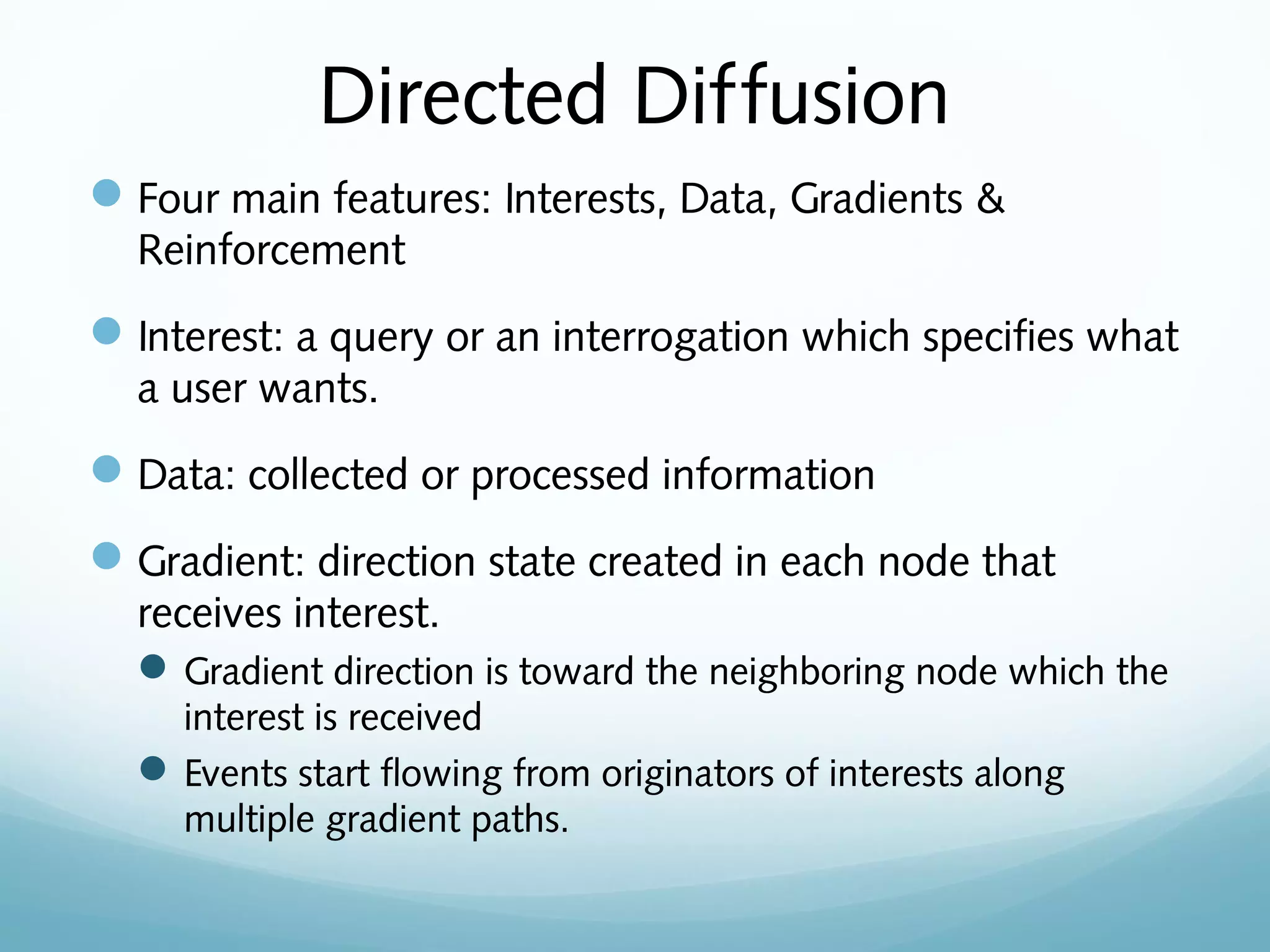
Overview of directed diffusion components like interests, data, and gradients for efficient communication.
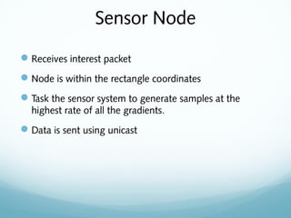
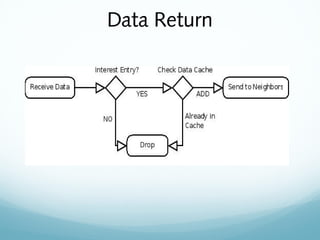
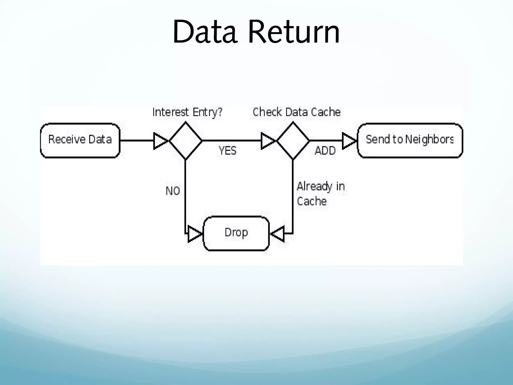
How sensor nodes manage interest packets and return data, including tasks for efficient sampling.
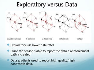
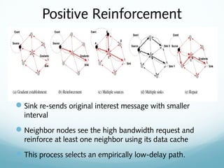
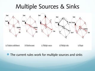
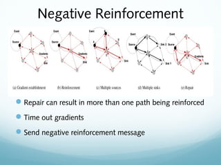
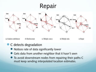
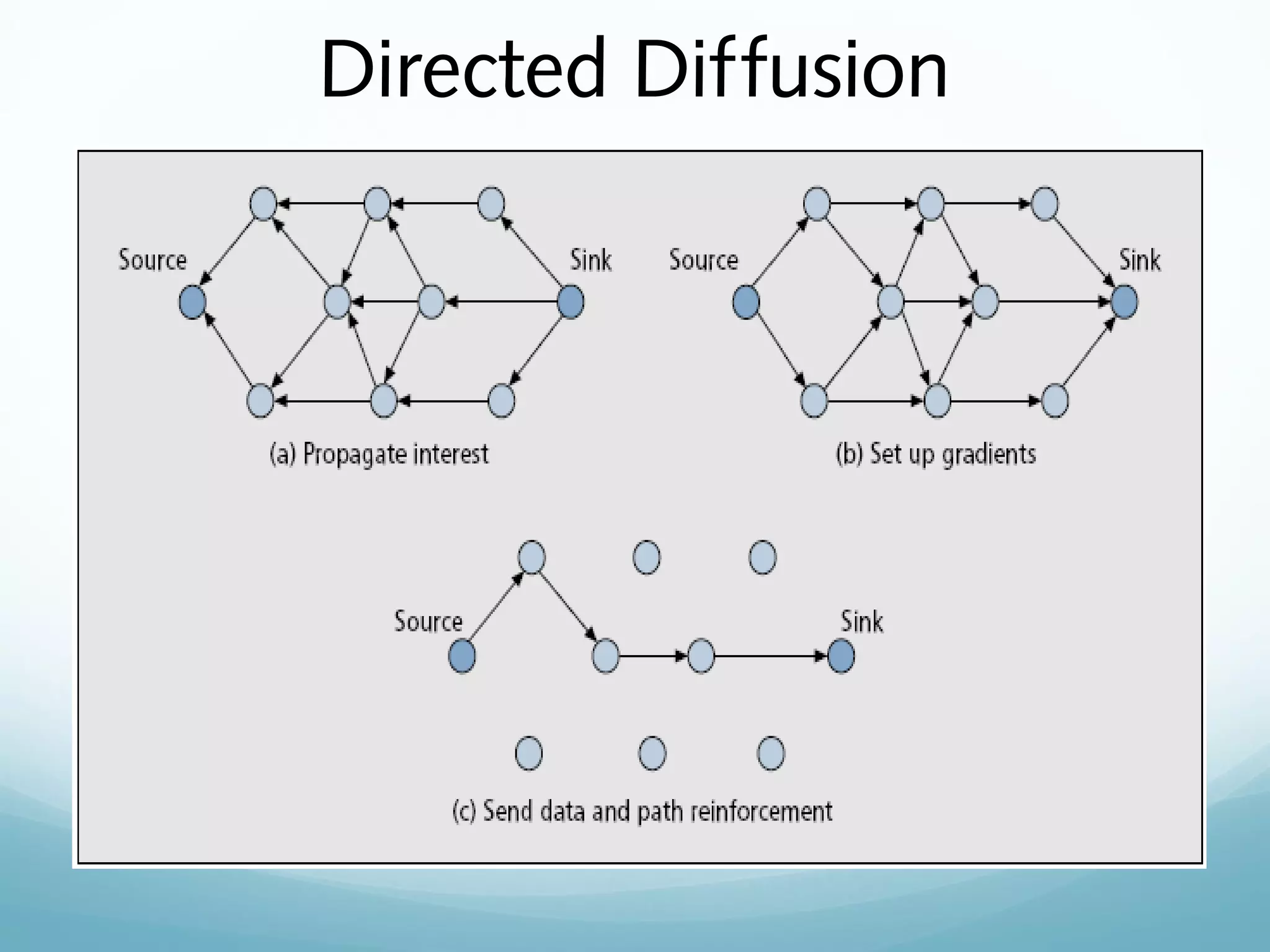
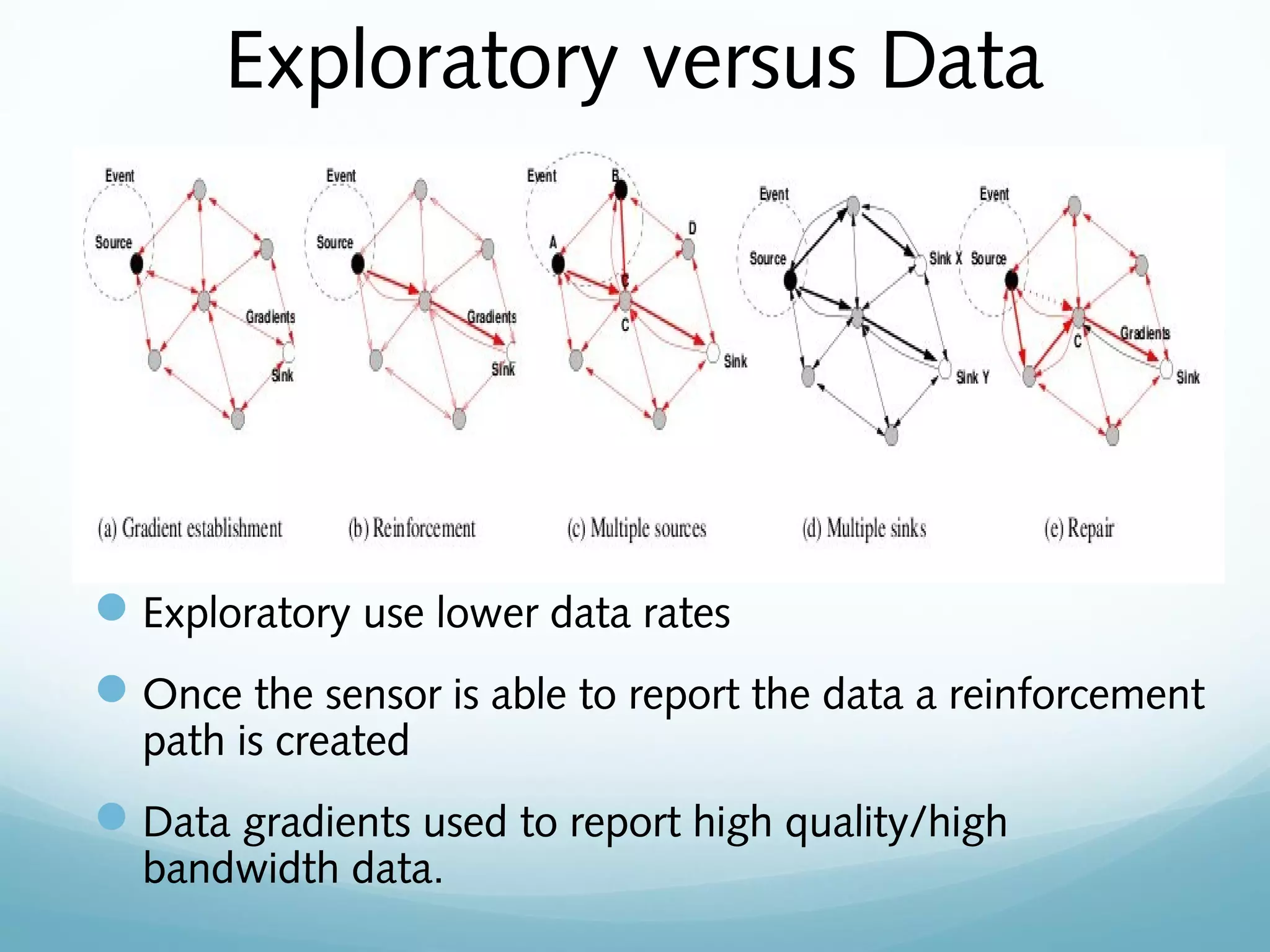
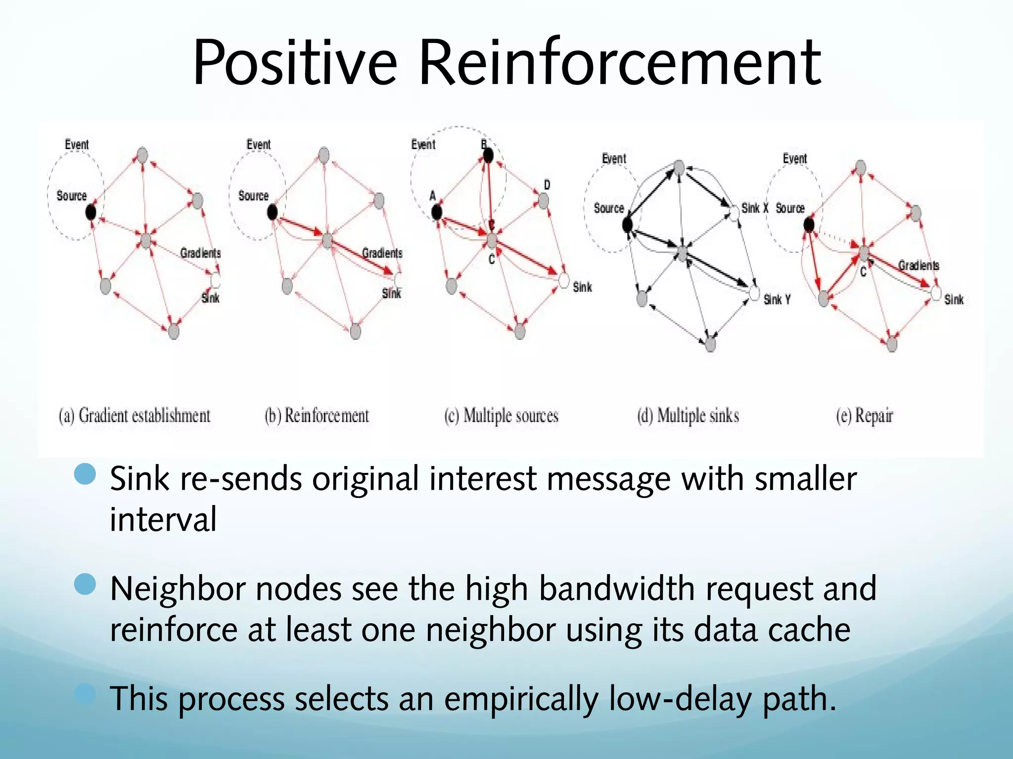
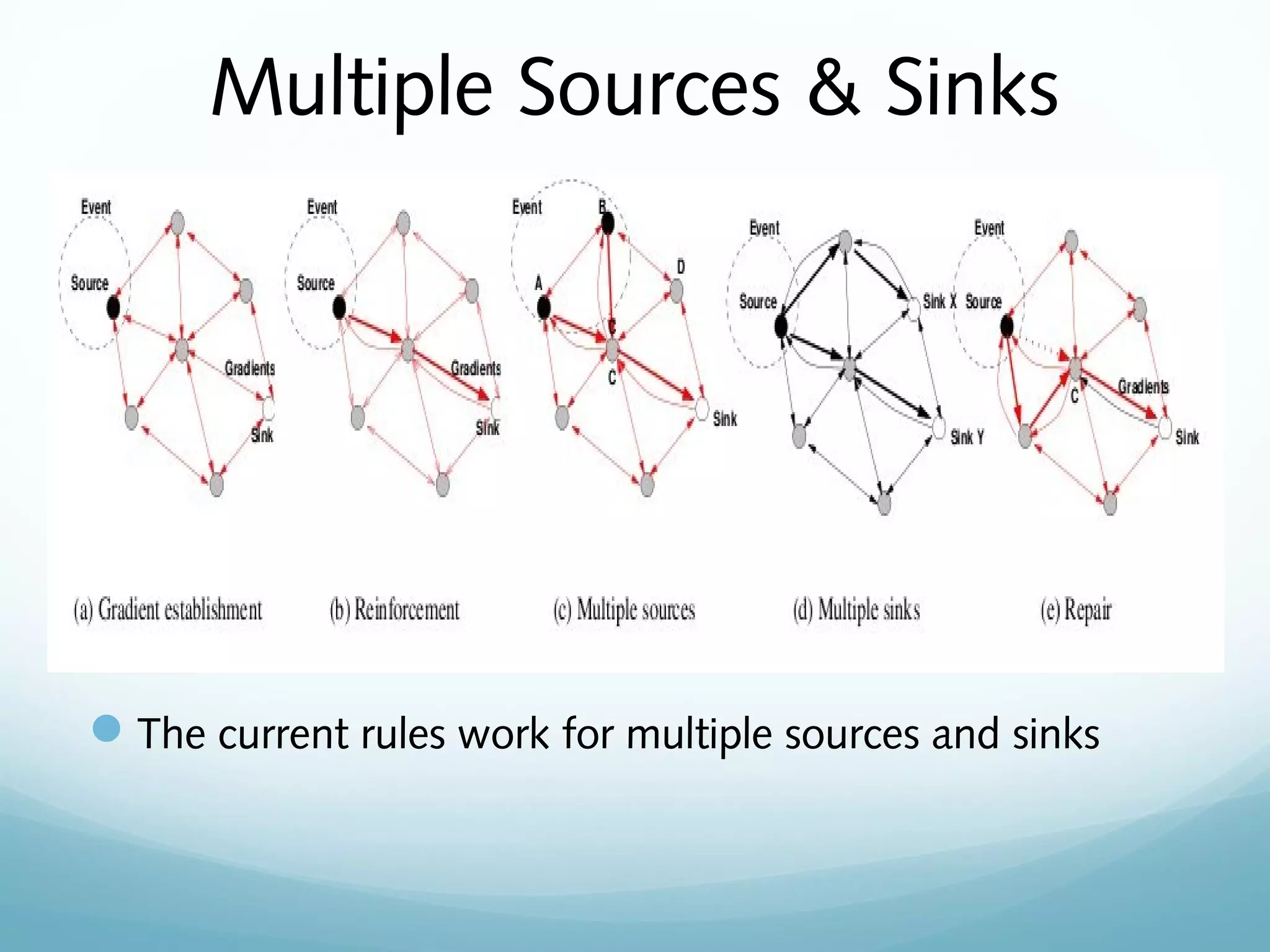
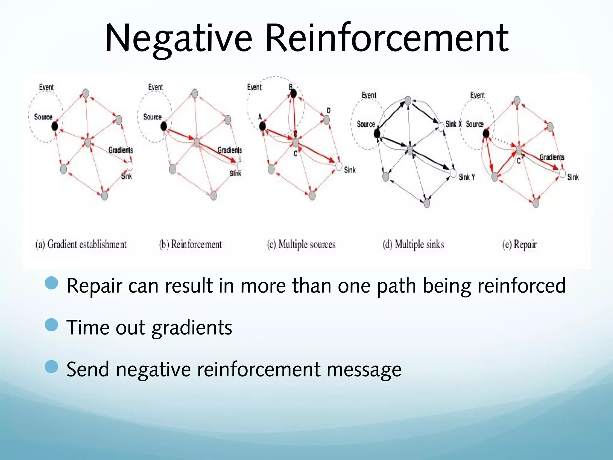
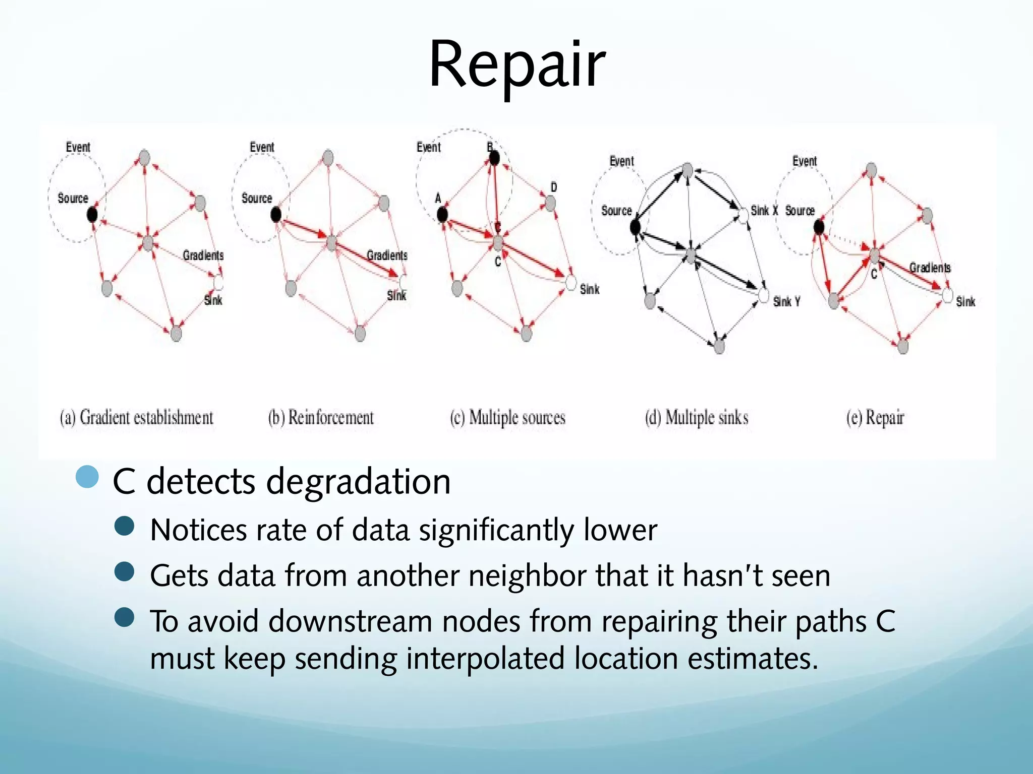
Discussion on exploratory data versus full data pathways, reinforcement methods, and repair techniques.
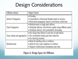
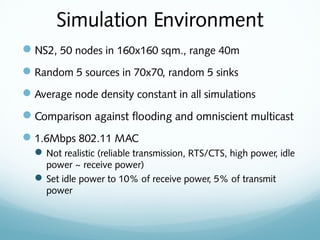
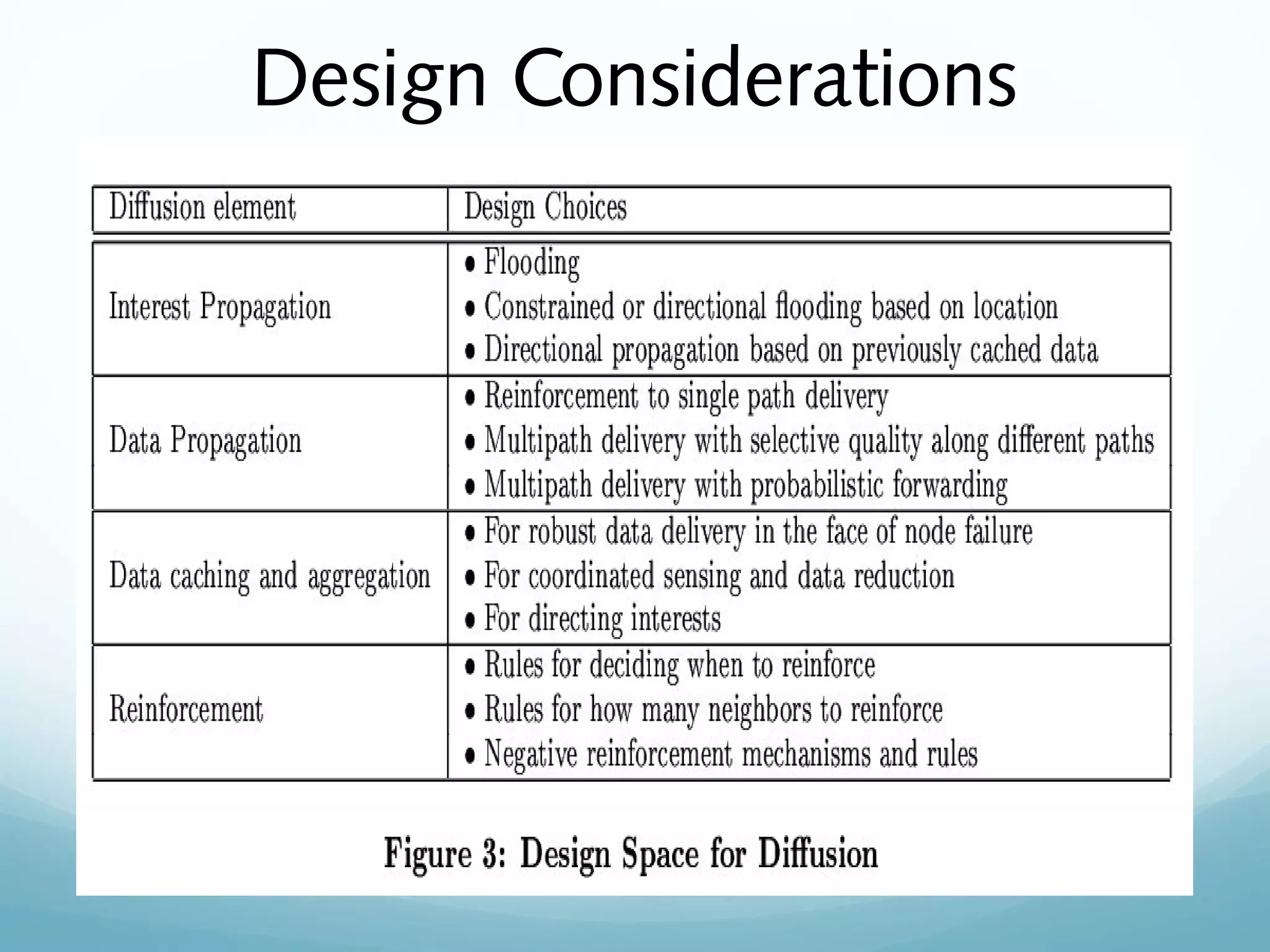
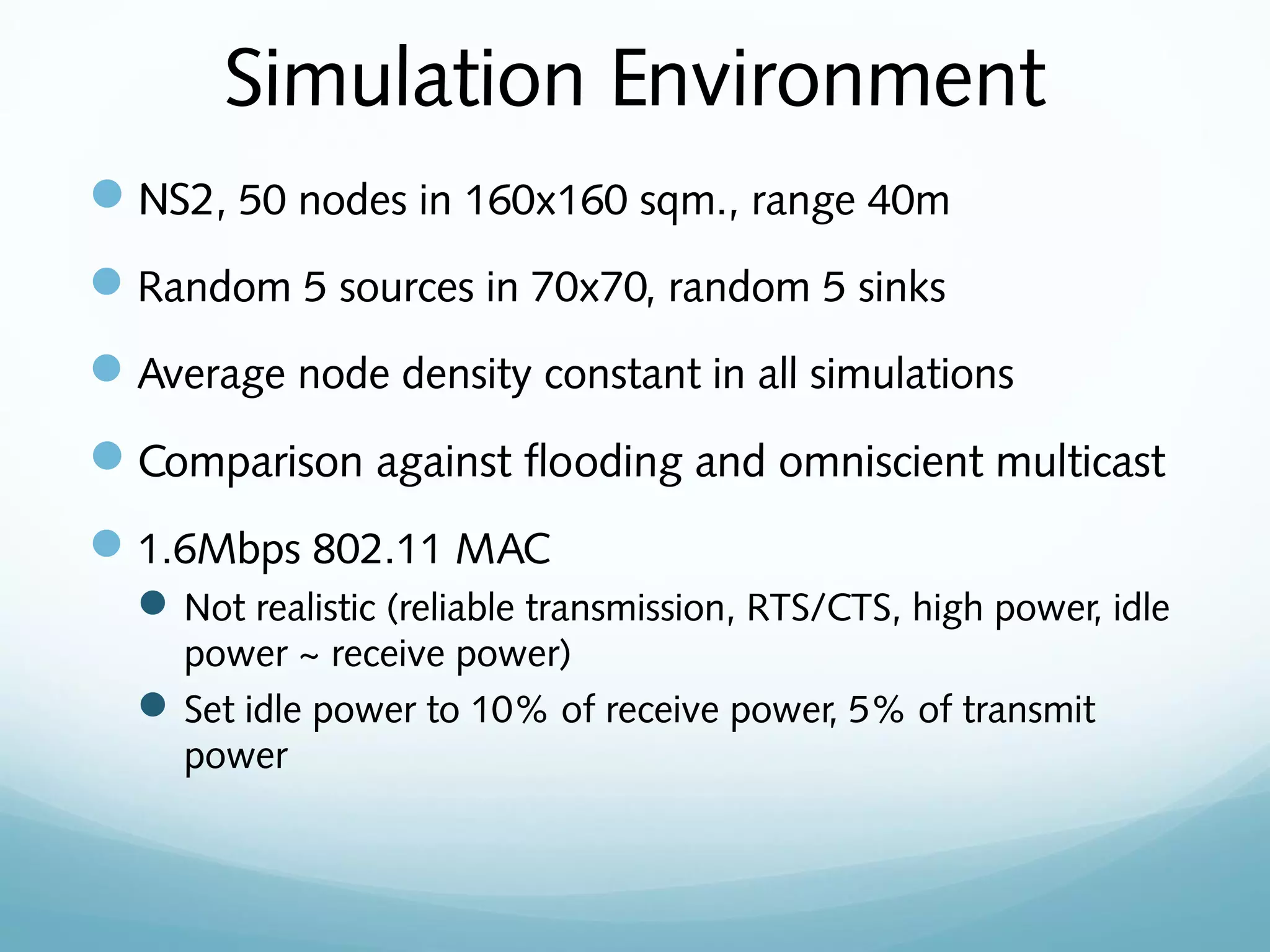
Design considerations and simulation environments used to test directed diffusion with various metrics.
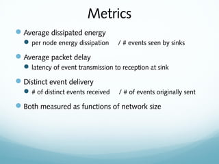
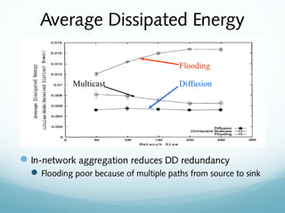
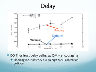
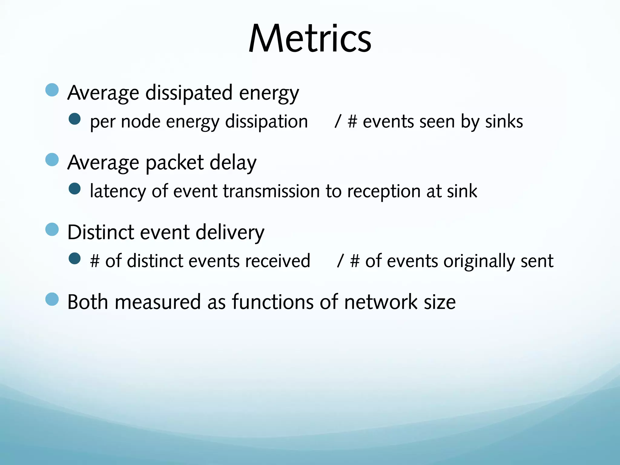
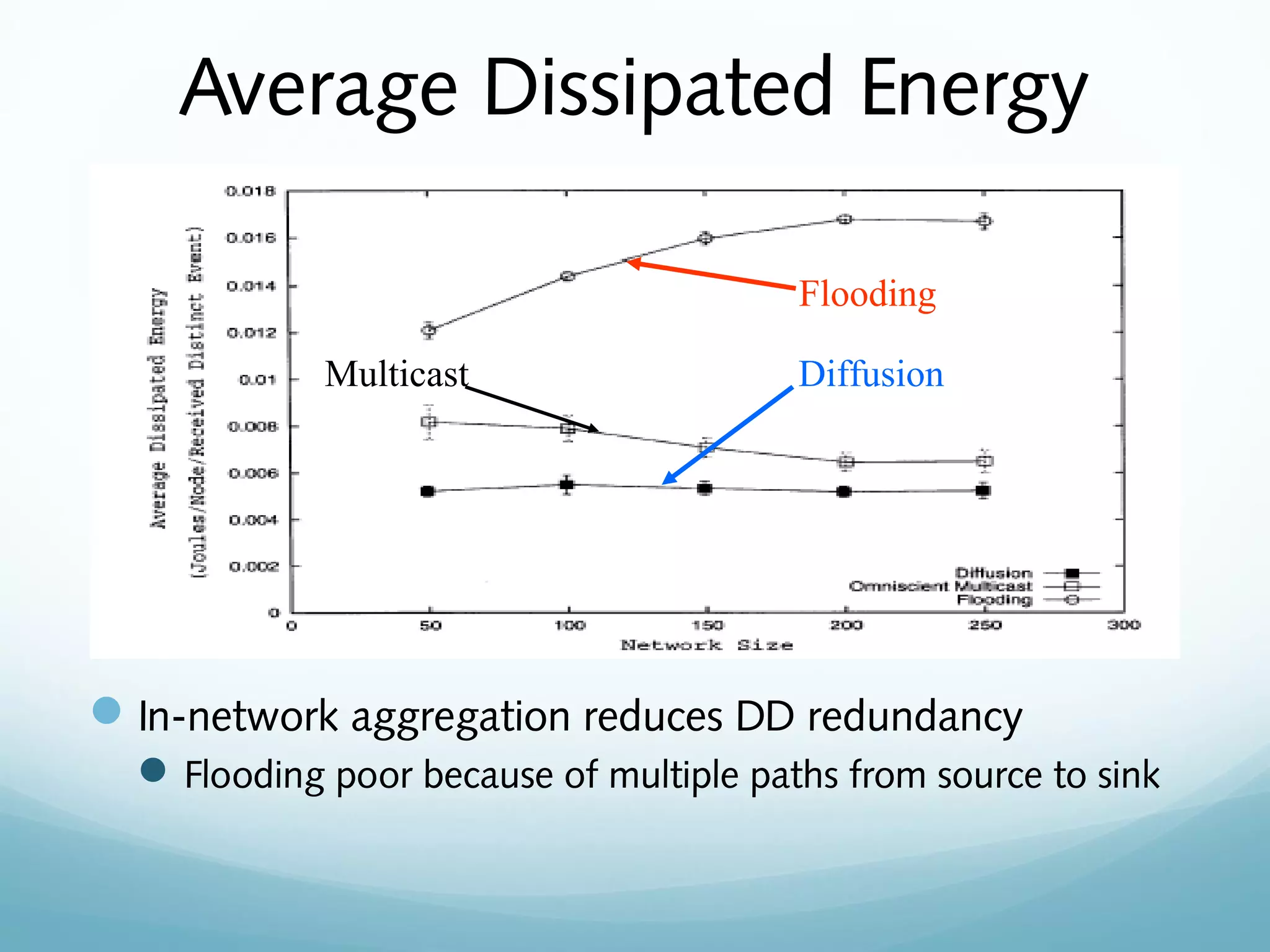
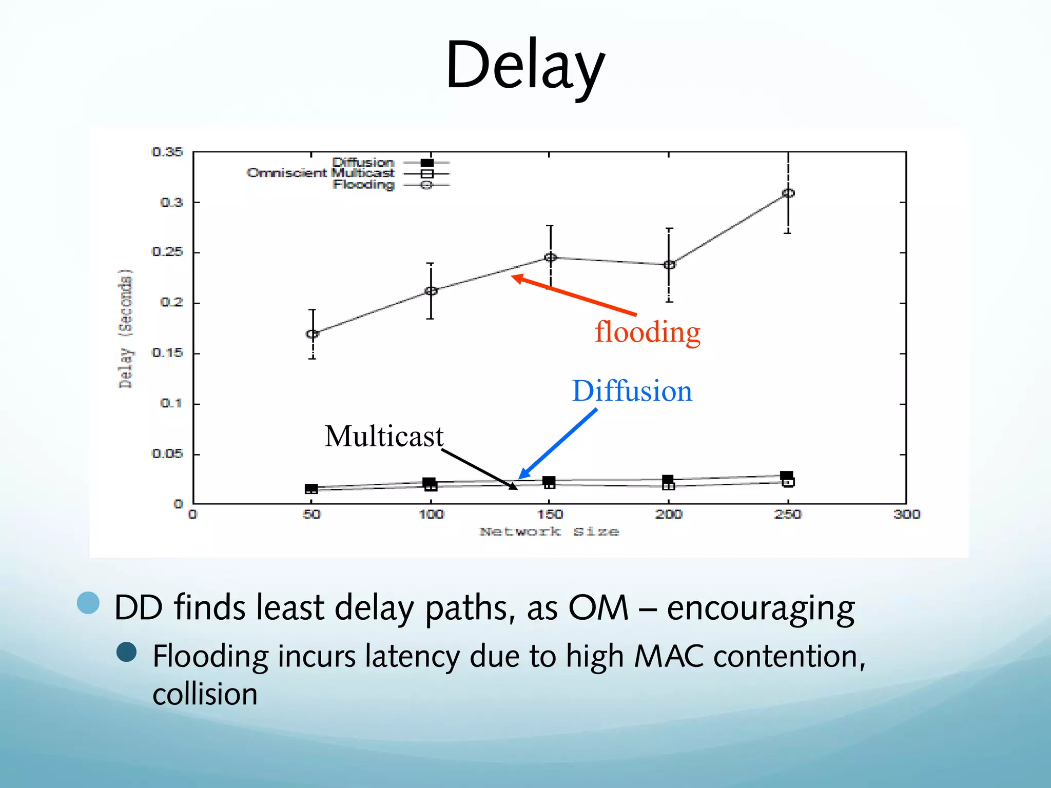
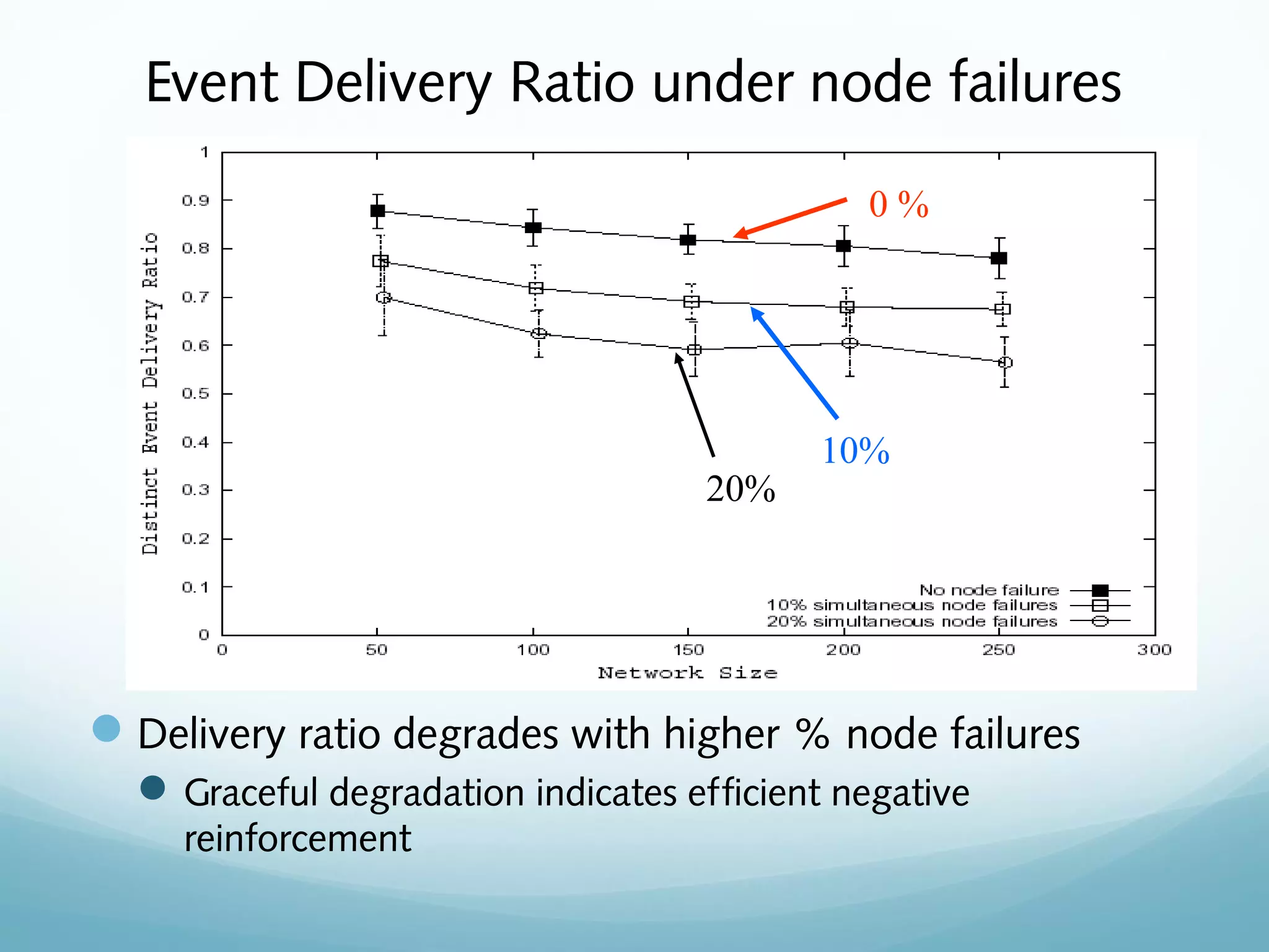
Metrics evaluation including average energy dissipation, packet delay, and delivery ratio in various scenarios.
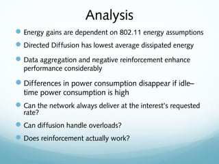
Pros and cons of directed diffusion in sensor networks and its resilience, noting areas for further study.
Final thoughts on directed diffusion, emphasizing energy efficiency and the need for improved MAC protocols.


