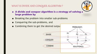
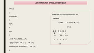
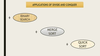
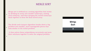
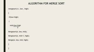
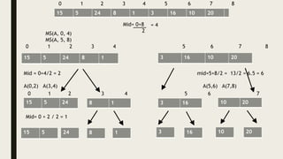
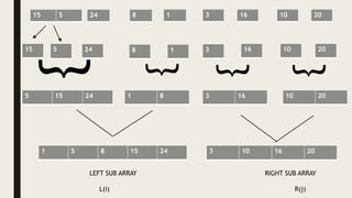
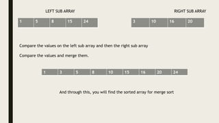
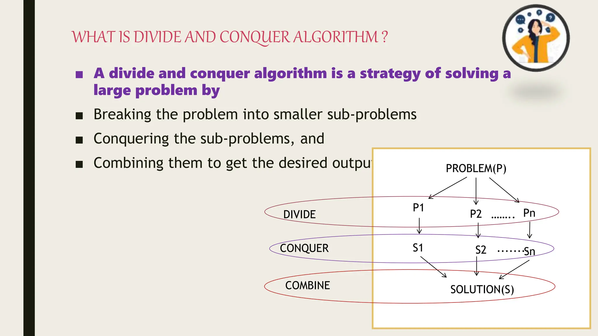
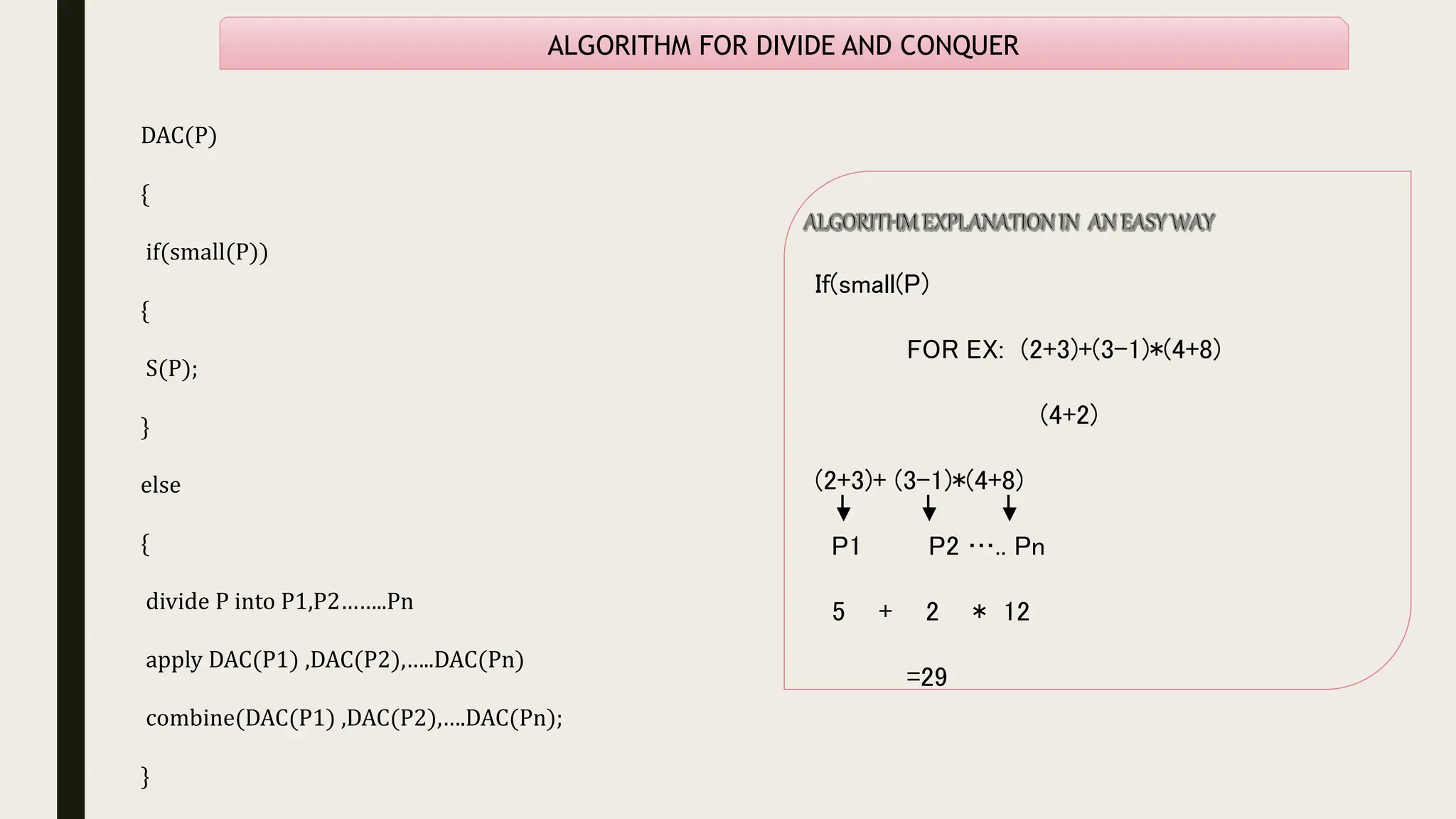
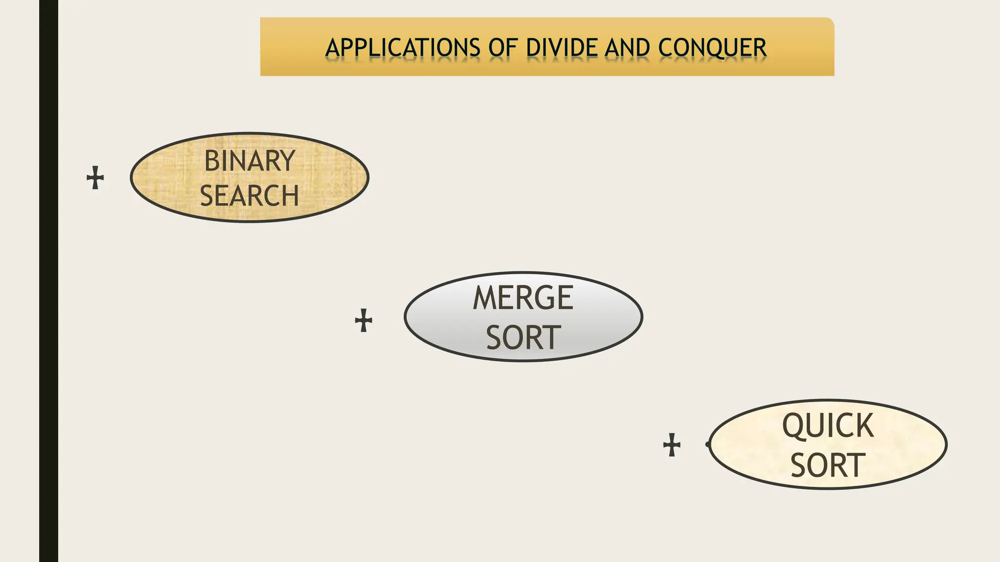
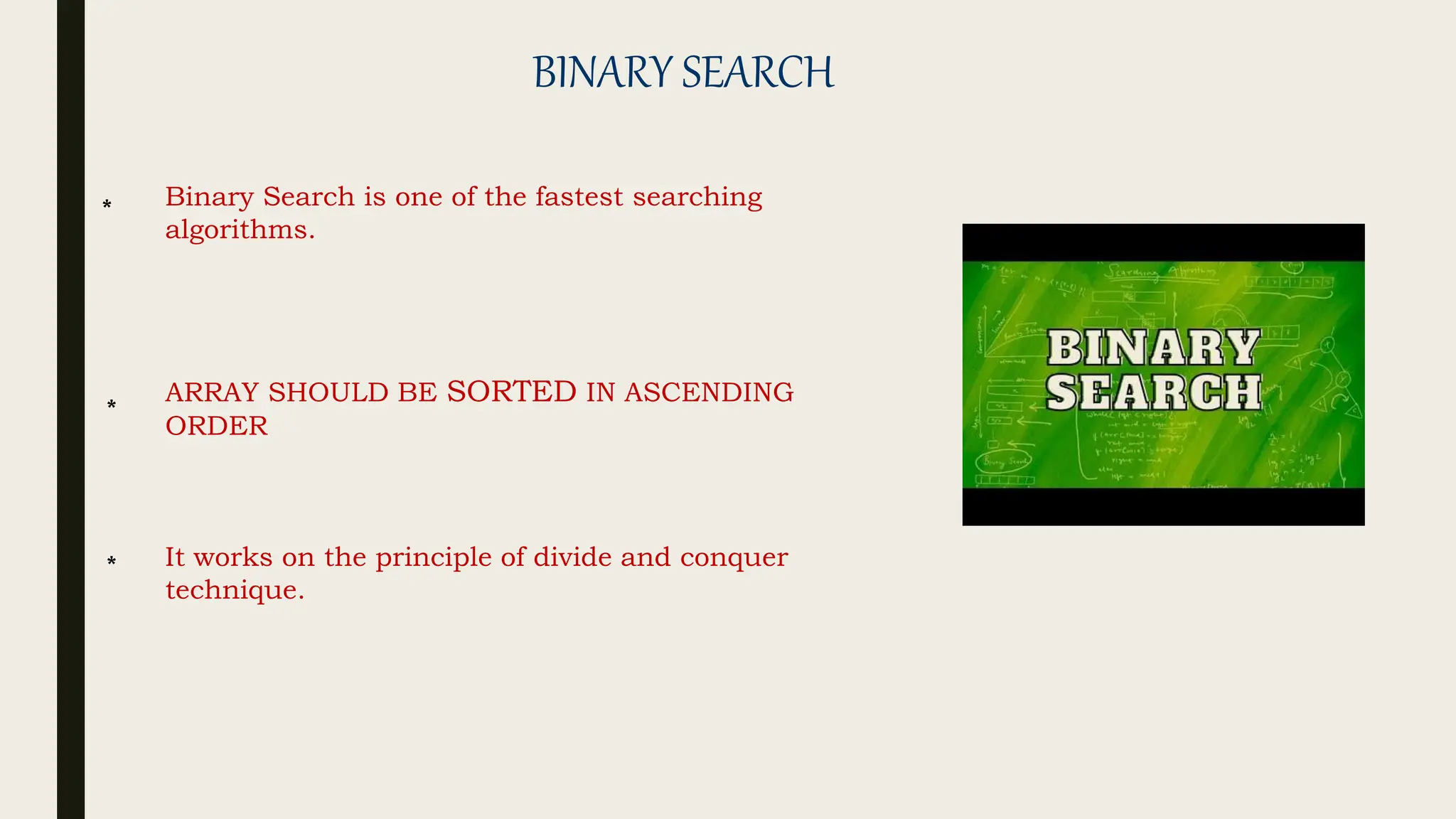
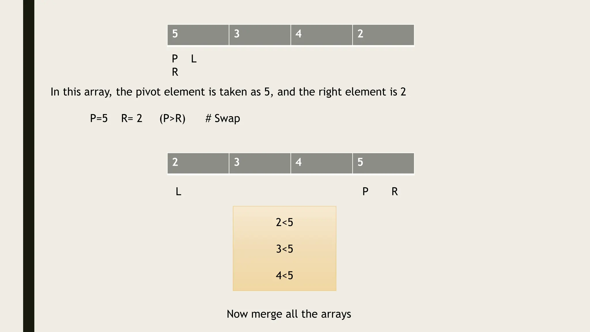
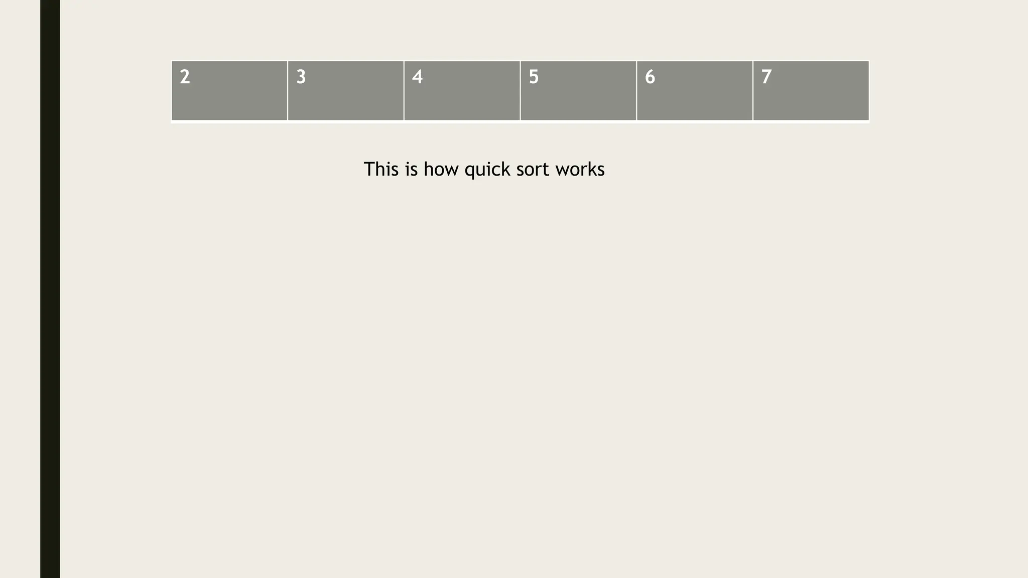
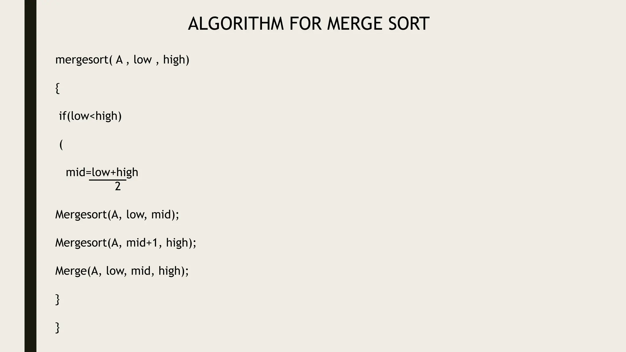
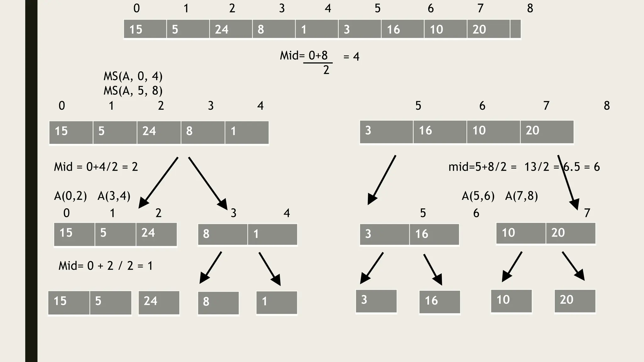
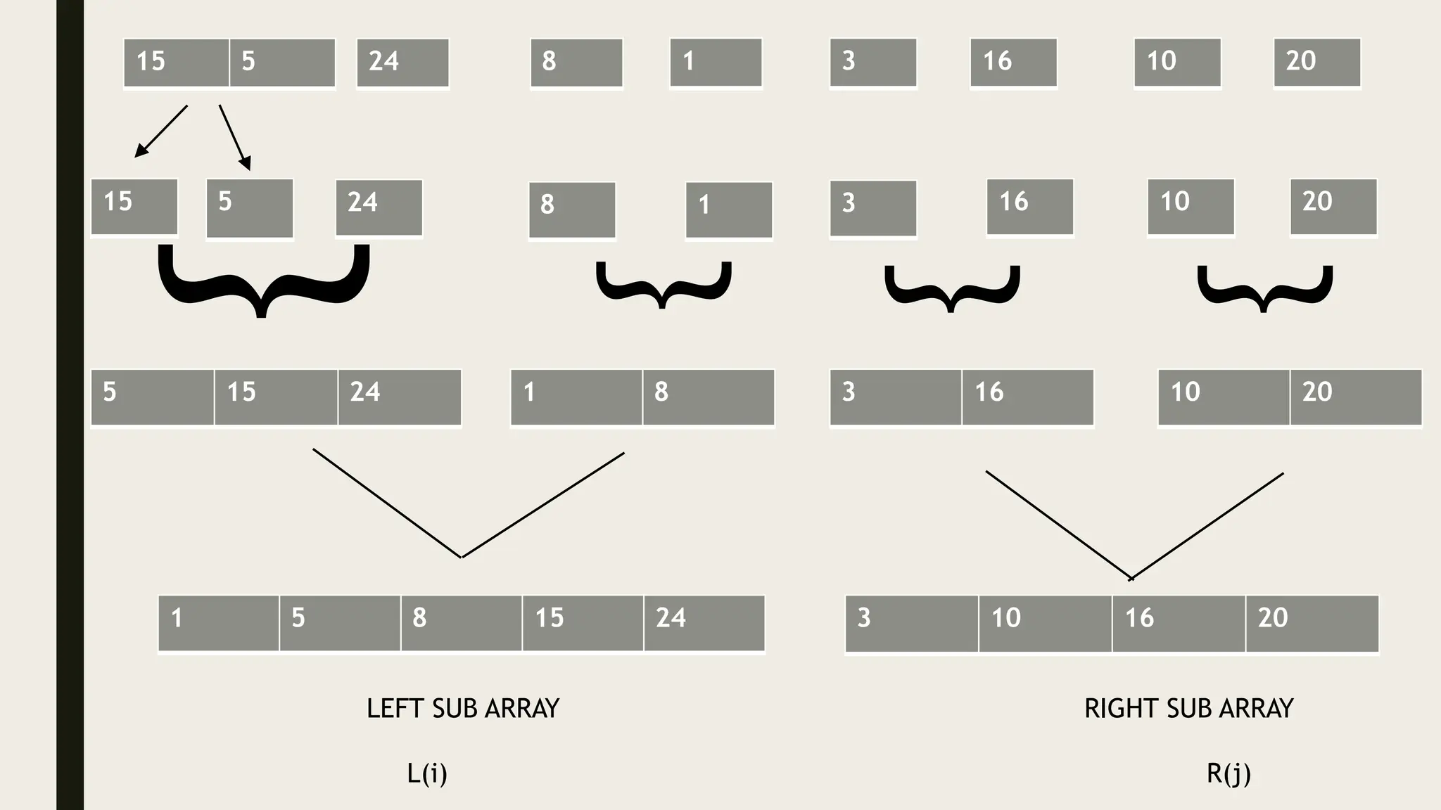
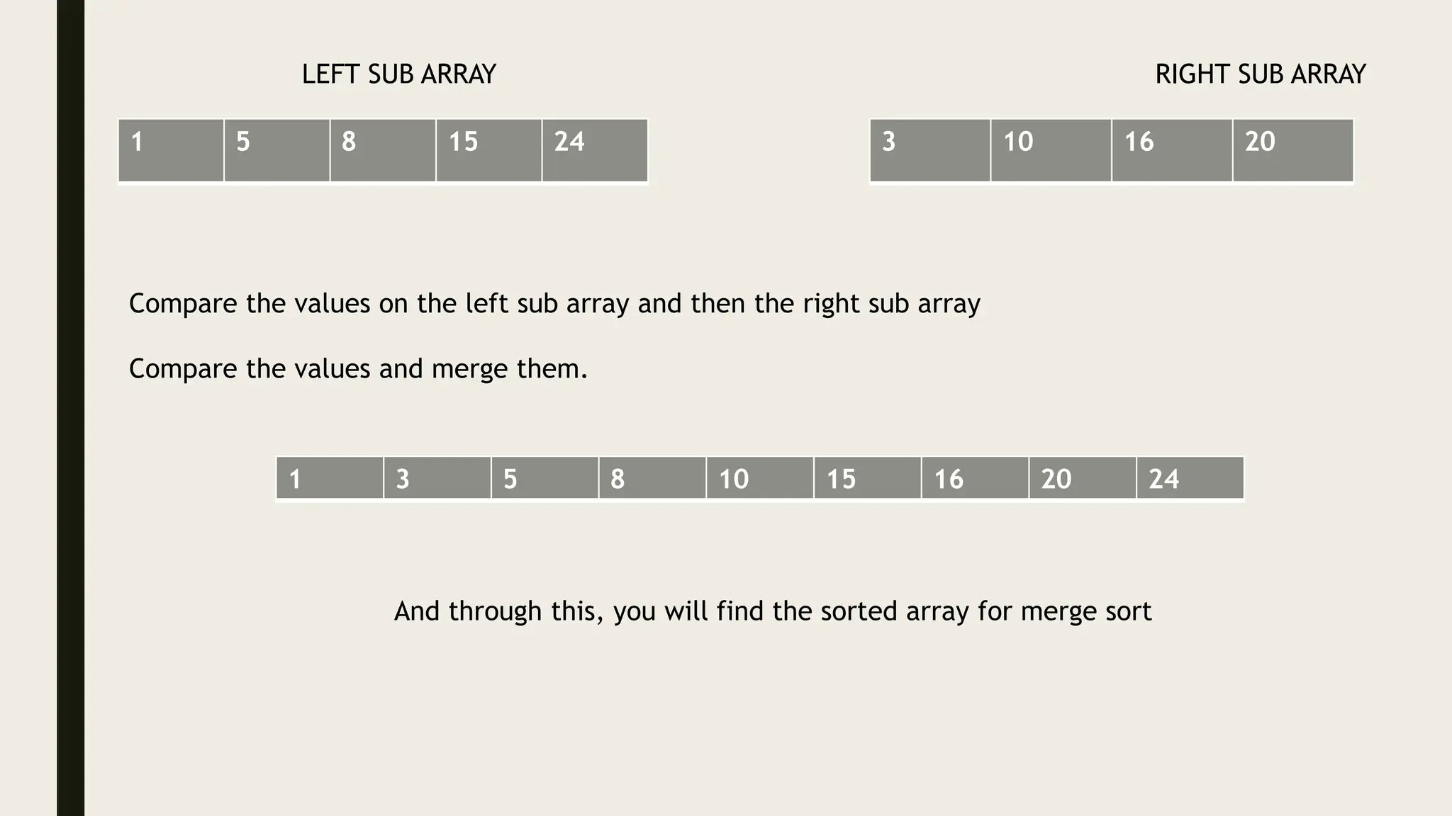
KEMBAR78
DIVIDE AND CONQUERMETHOD IN DATASTRUCTURE.pptx
By,
LAKSHMI.S, MCA,M.PHIL,
ASSISTANT PROFESSOR,
DEPARTMENT OF COMPUTER SCIENCE,
SRI ADI CHUNCHANAGIRI WOMENS COLLEGE, CUMBUM.
DIVIDE AND CONQUER METHOD
WHAT IS DIVIDE AND CONQUER ALGORITHM ?
■ A divide and conquer algorithm is a strategy of solving a
large problem by
■ Breaking the problem into smaller sub-problems
■ Conquering the sub-problems, and
■ Combining them to get the desired output. PROBLEM(P)
P1
P2 Pn
……..
S1 S2 Sn
........
SOLUTION(S)
DIVIDE
CONQUER
COMBINE
.
How Divide and Conquer Algorithms Work?
Here are the steps involved:
DIVIDE : Divide the given problem into sub-problems using recursion.
CONQUER : Solve the smaller sub-problems recursively. If the subproblem is small
enough, then solve it directly.
COMBINE : Combine the solutions of the sub-problems that are part of the recursive
process to solve the actual problem
ALGORITHM FOR DIVIDE AND CONQUER
DAC(P)
{
if(small(P))
{
S(P);
}
else
{
divide P into P1,P2……..Pn
apply DAC(P1) ,DAC(P2),…..DAC(Pn)
combine(DAC(P1) ,DAC(P2),….DAC(Pn);
}
If(small(P)
FOR EX: (2+3)+(3-1)*(4+8)
(4+2)
(2+3)+ (3-1)*(4+8)
P1 P2 ….. Pn
5 + 2 * 12
=29
QUICK
SORT
MERGE
SORT
BINARY
SEARCH
BINARY SEARCH
Binary Search is one of the fastest searching
algorithms.
ARRAY SHOULD BE SORTED IN ASCENDING
ORDER
It works on the principle of divide and conquer
technique.
*
*
*
ALGORITHM FOR BINARY SEARCH
binarysearch(a, n, key)
start=0, end= n-1
while(start<=end)
{
mid=start+end ;
2
if(key==a[mid])
return mid;
else if(key<a[mid])
end=mid-1;
else
start=mid+1;
} #end of loop
return -1; #start>end
} unsuccessful search
5 9 17 23 25 45 59 63 71 89
0 1 2 3 4 5 6 7 8 9
start end
KEY=59 #element to be found
m=10
EXAMPLE OF BINARY SEARCH
mid=start+end
2
=0+9/2
=4.5 => 4
So the mid value is 4
a[mid] = a[4] = 25
KEY= MID
KEY< MID -> END=MID-1
KEY>MID -> START=MID+1
And here now, as the key value is greater than the mid value,
Start = mid +1
= 4 +1
= 5
59>25
45 59 63 71 89
5 6 7 8 9
Start End
Mid = start + end = 5+9 = 14 = 7
2 2 2
a[mid]= 7 = 63
Here the key value is lesser than the mid value,
end = mid – 1
= 7 - 1
= 6
59<63
45 59
5 6
Start end
Mid= 5+6/2 = 11/2 = 5.5 = 5
a[mid]=45
Now the mid value is lesser than the key value,
Start= mid+ 1
= 5 + 1
= 6
45<59
59
6
Start end
Mid = 6 + 6
2
= 6 a[mid] = a[6] = 59
As key = mid
return mid
FINALLY THE KEY VALUE IS FOUND USING BINARY SEARCH
QUICK SORT
Quicksort is a divide-and-conquer algorithm.
It works by selecting a 'pivot' element from the
array and partitioning the other elements into two
sub-arrays, according to whether they are less than
or greater than the pivot.
For this reason, it is sometimes called partition-
exchange sort.
The key process in quick Sort is a partition()
*
*
*
*
THE RIGHT
SIDE MUST BE
GREATER
THAN PIVOT
THE LEFT
SIDE MUST BE
LESSER THAN
PIVOT
PIVOT CONDITION
LET US UNDERSTAND THROUGH AN EXAMPLE:
6 3 7 2 4 5
L R
PIVOT
CASE 1 :
Here the right side element is lesser than the pivot (ie)., P>R
P = 6 R = 5
In this condition, we need to swap the elements
6 3 7 2 4 5
5 3 7 2 4 6
L P
R
Case 2:
Here, now compare the left side element and the pivot element
L=5 P=6 (P>L) # no swap
5 3 7 2 4 6
Case 3:
Here, as the left element is moved to the next element (ie)., 3
Compare the pivot element and the left element
L=3 P=6(P>L) # no swap
L
P
R
5 3 7 2 4 6
L P
R
Case: 4
Now, the left element is moved to the next element, compare the element
with the pivot element…
L=7 P=6 (P<L)
In this condition, we need to swap.
5 3 6 2 4 7
P R
L
Case: 5
As the elements were swapped, now compare the pivot element with
the right side element…
P= 6 R=7 (P<R)
Here the pivot element is lesser than the right
Side, hence no swap
5 3 6 2 4 7
Case:6
Here the pivot element is greater than the
right side element P>R
P=6 R=4 #SWAP
P R
L
Case: 7
Now the swapping takes place, let’s compare
the pivot element with the left side element
P=6 L=4 (P>L) #no swap
5 3 4 2 6 7
P
L
R
Case:8
Here the pivot is greater than the left side
element
P=6 L=2 #no swap
FINALLY, We get the array
L P
R
Apply the quick sort on the rounded parts
5 3 4 2
P L
R
In this array, the pivot element is taken as 5, and the right element is 2
P=5 R= 2 (P>R) # Swap
2 3 4 5
P R
L
2<5
3<5
4<5
Now merge all the arrays
2 3 4 5 6 7
This is how quick sort works
MERGE SORT
The divide-and-conquer algorithm breaks down a big
problem into smaller, more manageable pieces that
look similar to the initial problem.
It then solves these subproblems recursively and puts
their solutions together to solve the original problem.
Merge sort is defined as a sorting algorithm that works
by dividing an array into smaller subarrays, sorting
each subarray, and then merging the sorted subarrays
back together to form the final sorted array.
*
*
*
ALGORITHM FOR MERGE SORT
mergesort( A , low , high)
{
if(low<high)
(
mid=low+high
2
Mergesort(A, low, mid);
Mergesort(A, mid+1, high);
Merge(A, low, mid, high);
}
}
Mid= 0+8
2
= 4
MS(A, 0, 4)
MS(A, 5, 8)
15 5 24 8 1 3 16 10 20
0 1 2 3 4 5 6 7 8
Mid = 0+4/2 = 2 mid=5+8/2 = 13/2 = 6.5 = 6
A(0,2) A(3,4) A(5,6) A(7,8)
15 5 24 8 1 3 16 10 20
Mid= 0 + 2 / 2 = 1
15 5 24 8 1 3 16 10 20
15 5 24 8 1 3 16 10 20
0 1 2 3 4 5 6 7 8
0 1 2 3 4 5 6 7
15 5 24 8 1 3 16 20
10
20
10
16
3
1
8
24
5
15
{
5 15 24 1 8 3 16 10 20
{
{
{
1 5 8 15 24 3 10 16 20
LEFT SUB ARRAY RIGHT SUB ARRAY
L(i) R(j)
1 5 8 15 24 3 10 16 20
LEFT SUB ARRAY RIGHT SUB ARRAY
Compare the values on the left sub array and then the right sub array
Compare the values and merge them.
1 3 5 8 10 15 16 20 24
And through this, you will find the sorted array for merge sort
DIVIDE AND CONQUERMETHOD IN DATASTRUCTURE.pptx

DIVIDE AND CONQUERMETHOD IN DATASTRUCTURE.pptx

  • 1.
    By, LAKSHMI.S, MCA,M.PHIL, ASSISTANT PROFESSOR, DEPARTMENTOF COMPUTER SCIENCE, SRI ADI CHUNCHANAGIRI WOMENS COLLEGE, CUMBUM. DIVIDE AND CONQUER METHOD
  • 2.
    WHAT IS DIVIDEAND CONQUER ALGORITHM ? ■ A divide and conquer algorithm is a strategy of solving a large problem by ■ Breaking the problem into smaller sub-problems ■ Conquering the sub-problems, and ■ Combining them to get the desired output. PROBLEM(P) P1 P2 Pn …….. S1 S2 Sn ........ SOLUTION(S) DIVIDE CONQUER COMBINE
  • 3.
    . How Divide andConquer Algorithms Work? Here are the steps involved: DIVIDE : Divide the given problem into sub-problems using recursion. CONQUER : Solve the smaller sub-problems recursively. If the subproblem is small enough, then solve it directly. COMBINE : Combine the solutions of the sub-problems that are part of the recursive process to solve the actual problem
  • 4.
    ALGORITHM FOR DIVIDEAND CONQUER DAC(P) { if(small(P)) { S(P); } else { divide P into P1,P2……..Pn apply DAC(P1) ,DAC(P2),…..DAC(Pn) combine(DAC(P1) ,DAC(P2),….DAC(Pn); } If(small(P) FOR EX: (2+3)+(3-1)*(4+8) (4+2) (2+3)+ (3-1)*(4+8) P1 P2 ….. Pn 5 + 2 * 12 =29
  • 5.
  • 6.
    BINARY SEARCH Binary Searchis one of the fastest searching algorithms. ARRAY SHOULD BE SORTED IN ASCENDING ORDER It works on the principle of divide and conquer technique. * * *
  • 7.
    ALGORITHM FOR BINARYSEARCH binarysearch(a, n, key) start=0, end= n-1 while(start<=end) { mid=start+end ; 2 if(key==a[mid]) return mid; else if(key<a[mid]) end=mid-1; else start=mid+1; } #end of loop return -1; #start>end } unsuccessful search
  • 8.
    5 9 1723 25 45 59 63 71 89 0 1 2 3 4 5 6 7 8 9 start end KEY=59 #element to be found m=10 EXAMPLE OF BINARY SEARCH mid=start+end 2 =0+9/2 =4.5 => 4 So the mid value is 4 a[mid] = a[4] = 25
  • 9.
    KEY= MID KEY< MID-> END=MID-1 KEY>MID -> START=MID+1 And here now, as the key value is greater than the mid value, Start = mid +1 = 4 +1 = 5 59>25 45 59 63 71 89 5 6 7 8 9 Start End Mid = start + end = 5+9 = 14 = 7 2 2 2 a[mid]= 7 = 63
  • 10.
    Here the keyvalue is lesser than the mid value, end = mid – 1 = 7 - 1 = 6 59<63 45 59 5 6 Start end Mid= 5+6/2 = 11/2 = 5.5 = 5 a[mid]=45
  • 11.
    Now the midvalue is lesser than the key value, Start= mid+ 1 = 5 + 1 = 6 45<59 59 6 Start end Mid = 6 + 6 2 = 6 a[mid] = a[6] = 59 As key = mid return mid FINALLY THE KEY VALUE IS FOUND USING BINARY SEARCH
  • 12.
    QUICK SORT Quicksort isa divide-and-conquer algorithm. It works by selecting a 'pivot' element from the array and partitioning the other elements into two sub-arrays, according to whether they are less than or greater than the pivot. For this reason, it is sometimes called partition- exchange sort. The key process in quick Sort is a partition() * * * *
  • 13.
    THE RIGHT SIDE MUSTBE GREATER THAN PIVOT THE LEFT SIDE MUST BE LESSER THAN PIVOT PIVOT CONDITION LET US UNDERSTAND THROUGH AN EXAMPLE: 6 3 7 2 4 5 L R PIVOT CASE 1 : Here the right side element is lesser than the pivot (ie)., P>R P = 6 R = 5 In this condition, we need to swap the elements 6 3 7 2 4 5
  • 14.
    5 3 72 4 6 L P R Case 2: Here, now compare the left side element and the pivot element L=5 P=6 (P>L) # no swap 5 3 7 2 4 6 Case 3: Here, as the left element is moved to the next element (ie)., 3 Compare the pivot element and the left element L=3 P=6(P>L) # no swap L P R
  • 15.
    5 3 72 4 6 L P R Case: 4 Now, the left element is moved to the next element, compare the element with the pivot element… L=7 P=6 (P<L) In this condition, we need to swap. 5 3 6 2 4 7 P R L Case: 5 As the elements were swapped, now compare the pivot element with the right side element… P= 6 R=7 (P<R) Here the pivot element is lesser than the right Side, hence no swap
  • 16.
    5 3 62 4 7 Case:6 Here the pivot element is greater than the right side element P>R P=6 R=4 #SWAP P R L Case: 7 Now the swapping takes place, let’s compare the pivot element with the left side element P=6 L=4 (P>L) #no swap 5 3 4 2 6 7 P L R
  • 17.
    Case:8 Here the pivotis greater than the left side element P=6 L=2 #no swap FINALLY, We get the array L P R Apply the quick sort on the rounded parts
  • 18.
    5 3 42 P L R In this array, the pivot element is taken as 5, and the right element is 2 P=5 R= 2 (P>R) # Swap 2 3 4 5 P R L 2<5 3<5 4<5 Now merge all the arrays
  • 19.
    2 3 45 6 7 This is how quick sort works
  • 20.
    MERGE SORT The divide-and-conqueralgorithm breaks down a big problem into smaller, more manageable pieces that look similar to the initial problem. It then solves these subproblems recursively and puts their solutions together to solve the original problem. Merge sort is defined as a sorting algorithm that works by dividing an array into smaller subarrays, sorting each subarray, and then merging the sorted subarrays back together to form the final sorted array. * * *
  • 21.
    ALGORITHM FOR MERGESORT mergesort( A , low , high) { if(low<high) ( mid=low+high 2 Mergesort(A, low, mid); Mergesort(A, mid+1, high); Merge(A, low, mid, high); } }
  • 22.
    Mid= 0+8 2 = 4 MS(A,0, 4) MS(A, 5, 8) 15 5 24 8 1 3 16 10 20 0 1 2 3 4 5 6 7 8 Mid = 0+4/2 = 2 mid=5+8/2 = 13/2 = 6.5 = 6 A(0,2) A(3,4) A(5,6) A(7,8) 15 5 24 8 1 3 16 10 20 Mid= 0 + 2 / 2 = 1 15 5 24 8 1 3 16 10 20 15 5 24 8 1 3 16 10 20 0 1 2 3 4 5 6 7 8 0 1 2 3 4 5 6 7
  • 23.
    15 5 248 1 3 16 20 10 20 10 16 3 1 8 24 5 15 { 5 15 24 1 8 3 16 10 20 { { { 1 5 8 15 24 3 10 16 20 LEFT SUB ARRAY RIGHT SUB ARRAY L(i) R(j)
  • 24.
    1 5 815 24 3 10 16 20 LEFT SUB ARRAY RIGHT SUB ARRAY Compare the values on the left sub array and then the right sub array Compare the values and merge them. 1 3 5 8 10 15 16 20 24 And through this, you will find the sorted array for merge sort