Downloaded 25 times


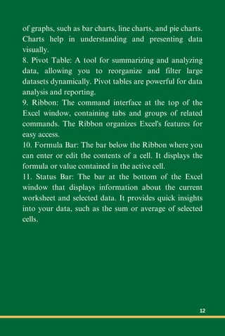
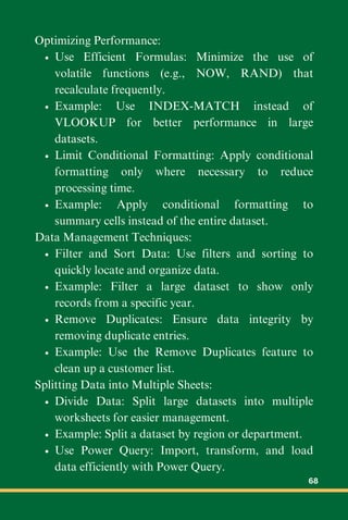
![Example Exercise:
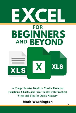
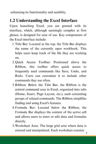
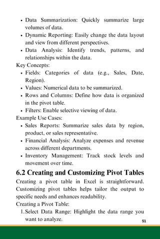
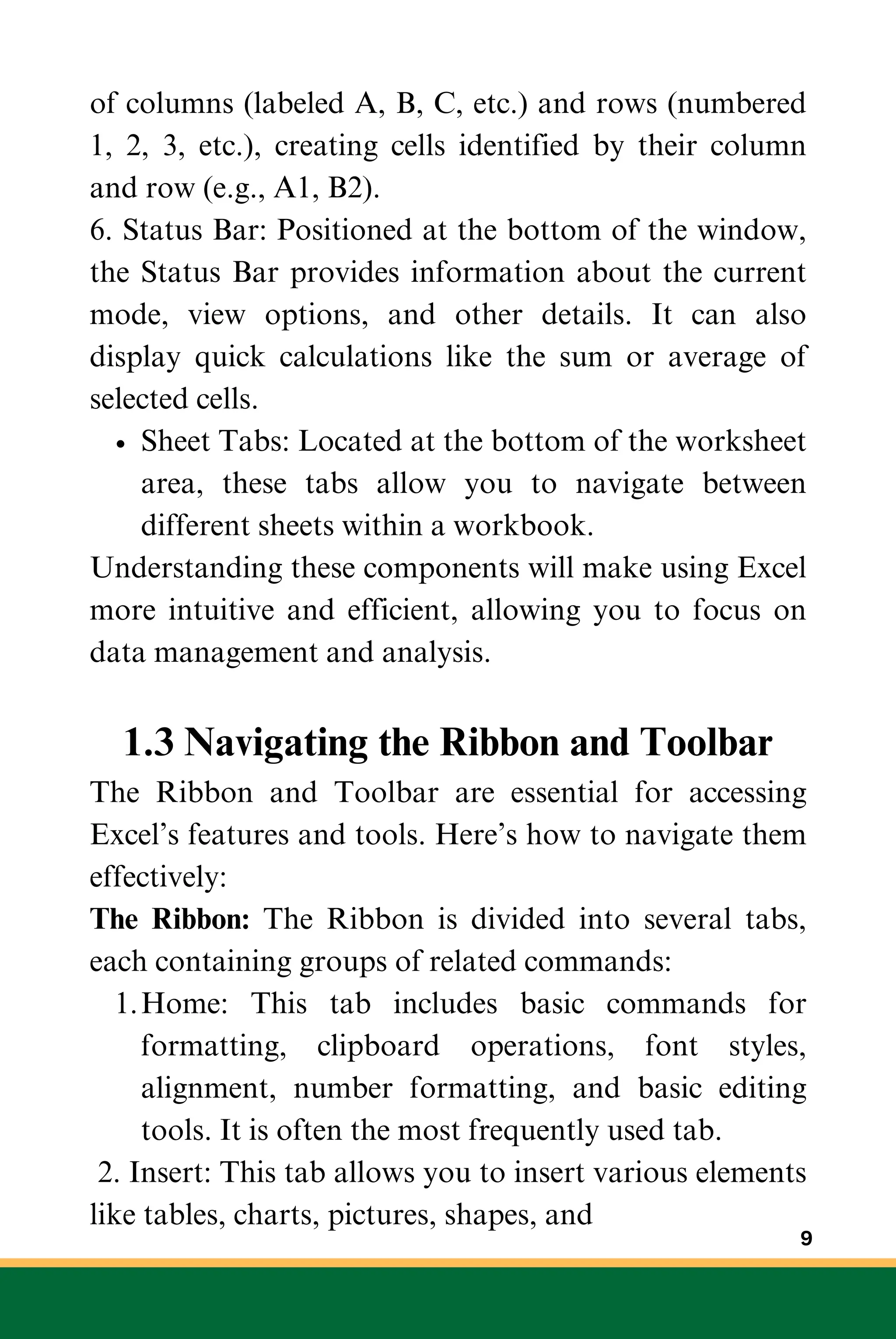
Let’s calculate the total, difference, product, and
quotient for a set of numbers:
Enter Data:
1.
In cell A1, type 5.
In cell B1, type 10.
Perform Arithmetic Operations:
2.
In cell C1, type =A1 + B1 (result: 15).
In cell D1, type =A1 - B1 (result: -5).
In cell E1, type =A1 * B1 (result: 50).
In cell F1, type =A1 / B1 (result: 0.5).
These basic arithmetic operations form the foundation
for more complex calculations and data analysis in
Excel.
2.3 Commonly Used Functions: SUM,
AVERAGE, MIN, MAX
Excel provides a range of functions for various
calculations. Some of the most commonly used
functions are SUM, AVERAGE, MIN, and MAX.
SUM: Adds all the numbers in a range of cells.
Syntax: =SUM(number1, [number2], ...)
Example: =SUM(A1:A10) adds all the numbers in
cells A1 through A10.
AVERAGE: Calculates the average (arithmetic mean)
of a range of numbers.
Syntax: =AVERAGE(number1, [number2], ...)
Example: =AVERAGE(A1:A10) calculates the 18](https://image.slidesharecdn.com/excelforbeginnersandbeyond-240827021017-eff1230a/85/Excel-for-Beginners-and-Beyond-Introduction-to-Excel-18-320.jpg)
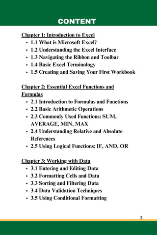
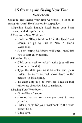
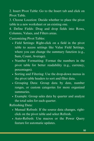
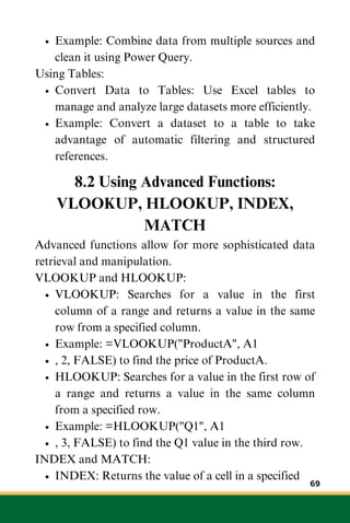
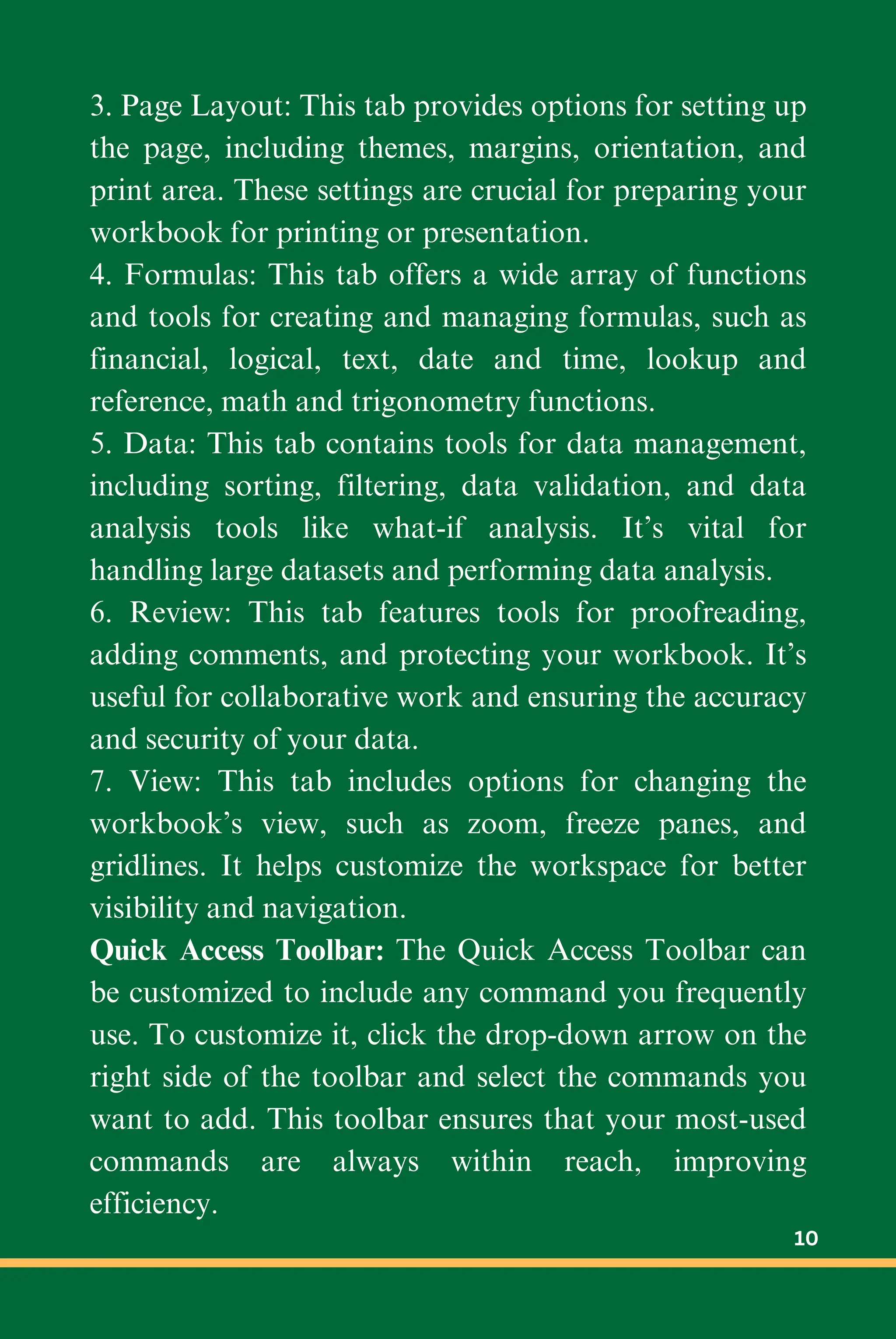
![average of the numbers in cells A1 through A10.
MIN: Returns the smallest number in a range of cells.
Syntax: =MIN(number1, [number2], ...)
Example: =MIN(A1:A10) finds the smallest
number in cells A1 through A10.
MAX: Returns the largest number in a range of cells.
Syntax: =MAX(number1, [number2], ...)
Example: =MAX(A1:A10) finds the largest number
in cells A1 through A10.
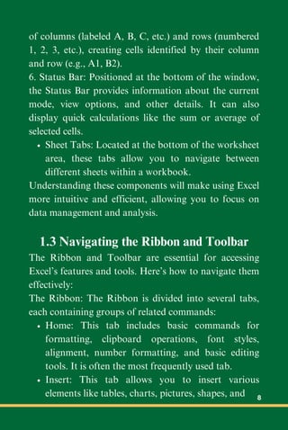
Example Exercise:
Let’s use these functions to summarize a set of data:
Enter Data:
In cells A1 through A5, enter the values 10, 20,
30, 40, 50.
Calculate SUM, AVERAGE, MIN, and MAX:
In cell B1, type =SUM(A1:A5) (result: 150).
In cell B2, type =AVERAGE(A1:A5) (result:
30).
In cell B3, type =MIN(A1:A5) (result: 10).
In cell B4, type =MAX(A1:A5) (result: 50).
These functions are essential for summarizing and
analyzing numerical data quickly.
2.4 Understanding Relative and Absolute
References
In Excel, cell references can be relative, absolute, or
mixed. Understanding these reference types is crucial
for creating formulas that work correctly when copied 19](https://image.slidesharecdn.com/excelforbeginnersandbeyond-240827021017-eff1230a/85/Excel-for-Beginners-and-Beyond-Introduction-to-Excel-19-320.jpg)
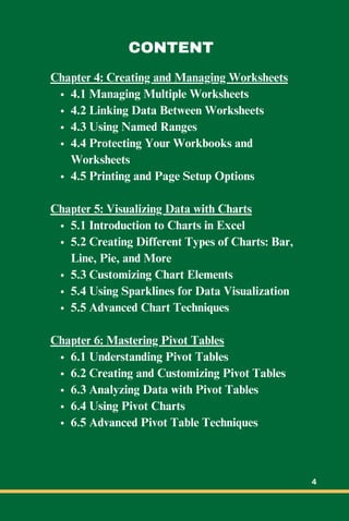
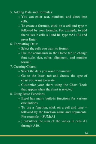
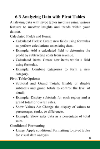
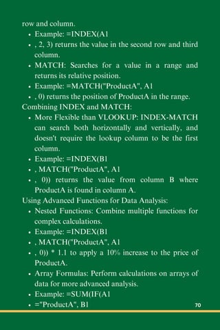
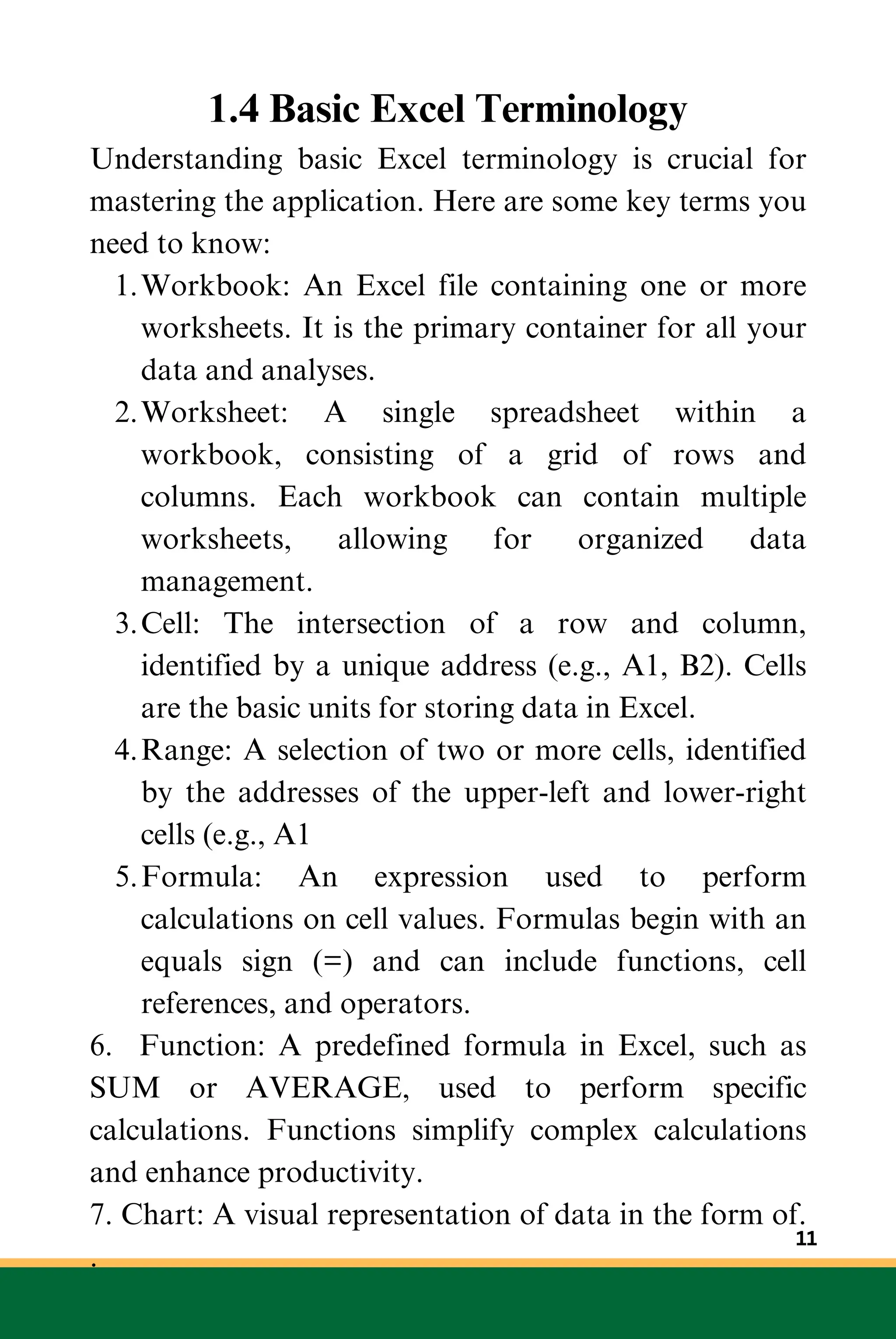
![Understanding how to use these references will help
you create flexible and robust formulas.
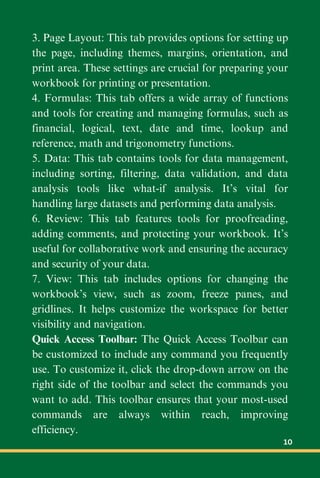
2.5 Using Logical Functions: IF, AND, OR
Logical functions allow you to perform conditional
operations based on specified criteria. The most
commonly used logical functions in Excel are IF,
AND, and OR.
IF: Returns one value if a condition is true and another
value if it is false.
Syntax: =IF(logical_test, value_if_true,
value_if_false)
Example: =IF(A1 > 10, "High", "Low") returns
"High" if the value in A1 is greater than 10,
otherwise returns "Low".
AND: Returns TRUE if all conditions are true, and
FALSE otherwise.
Syntax: =AND(logical1, [logical2], ...)
Example: =AND(A1 > 10, B1 < 5) returns TRUE
if both conditions are true.
OR: Returns TRUE if any condition is true, and
FALSE otherwise.
Syntax: =OR(logical1, [logical2], ...)
Example: =OR(A1 > 10, B1 < 5) returns TRUE if
either condition is true.
Example Exercise:
Let’s use logical functions to evaluate data:
21](https://image.slidesharecdn.com/excelforbeginnersandbeyond-240827021017-eff1230a/85/Excel-for-Beginners-and-Beyond-Introduction-to-Excel-21-320.jpg)


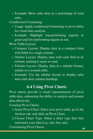


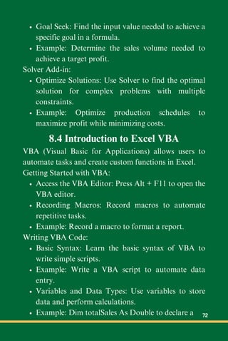


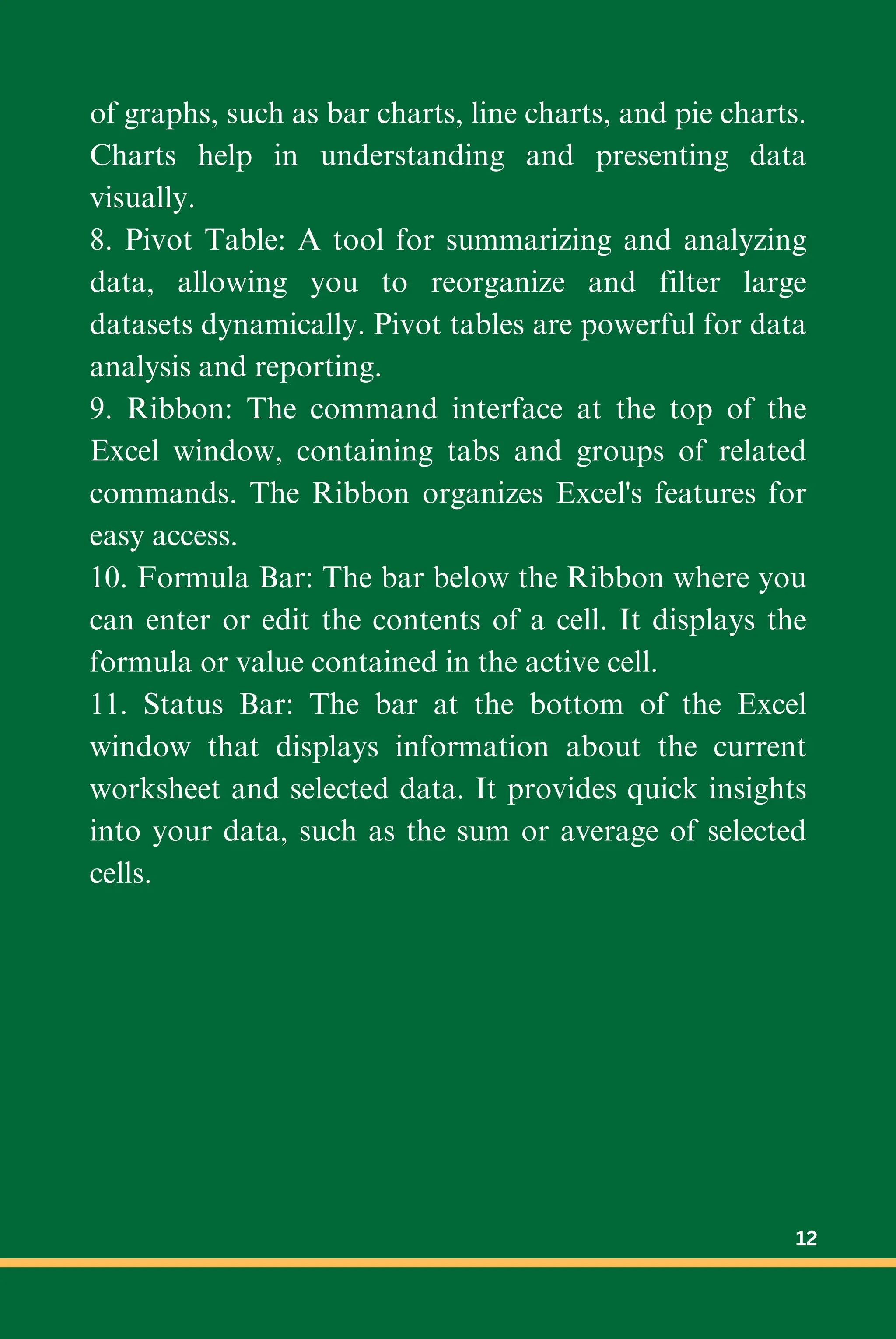

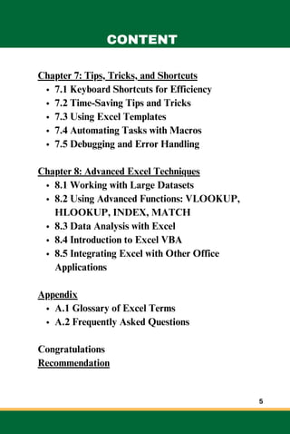
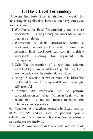
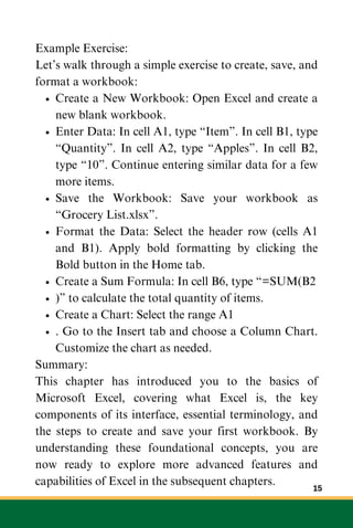
![Example Exercise:
Let’s calculate the total, difference, product, and
quotient for a set of numbers:
Enter Data:
1.
In cell A1, type 5.
In cell B1, type 10.
Perform Arithmetic Operations:
2.
In cell C1, type =A1 + B1 (result: 15).
In cell D1, type =A1 - B1 (result: -5).
In cell E1, type =A1 * B1 (result: 50).
In cell F1, type =A1 / B1 (result: 0.5).
These basic arithmetic operations form the foundation
for more complex calculations and data analysis in
Excel.
2.3 Commonly Used Functions: SUM,
AVERAGE, MIN, MAX
Excel provides a range of functions for various
calculations. Some of the most commonly used
functions are SUM, AVERAGE, MIN, and MAX.
SUM: Adds all the numbers in a range of cells.
Syntax: =SUM(number1, [number2], ...)
Example: =SUM(A1:A10) adds all the numbers in
cells A1 through A10.
AVERAGE: Calculates the average (arithmetic mean)
of a range of numbers.
Syntax: =AVERAGE(number1, [number2], ...)
Example: =AVERAGE(A1:A10) calculates the 18](https://image.slidesharecdn.com/excelforbeginnersandbeyond-240827021017-eff1230a/75/Excel-for-Beginners-and-Beyond-Introduction-to-Excel-18-2048.jpg)
![average of the numbers in cells A1 through A10.
MIN: Returns the smallest number in a range of cells.
Syntax: =MIN(number1, [number2], ...)
Example: =MIN(A1:A10) finds the smallest
number in cells A1 through A10.
MAX: Returns the largest number in a range of cells.
Syntax: =MAX(number1, [number2], ...)
Example: =MAX(A1:A10) finds the largest number
in cells A1 through A10.
Example Exercise:
Let’s use these functions to summarize a set of data:
Enter Data:
In cells A1 through A5, enter the values 10, 20,
30, 40, 50.
Calculate SUM, AVERAGE, MIN, and MAX:
In cell B1, type =SUM(A1:A5) (result: 150).
In cell B2, type =AVERAGE(A1:A5) (result:
30).
In cell B3, type =MIN(A1:A5) (result: 10).
In cell B4, type =MAX(A1:A5) (result: 50).
These functions are essential for summarizing and
analyzing numerical data quickly.
2.4 Understanding Relative and Absolute
References
In Excel, cell references can be relative, absolute, or
mixed. Understanding these reference types is crucial
for creating formulas that work correctly when copied 19](https://image.slidesharecdn.com/excelforbeginnersandbeyond-240827021017-eff1230a/75/Excel-for-Beginners-and-Beyond-Introduction-to-Excel-19-2048.jpg)
![Understanding how to use these references will help
you create flexible and robust formulas.
2.5 Using Logical Functions: IF, AND, OR
Logical functions allow you to perform conditional
operations based on specified criteria. The most
commonly used logical functions in Excel are IF,
AND, and OR.
IF: Returns one value if a condition is true and another
value if it is false.
Syntax: =IF(logical_test, value_if_true,
value_if_false)
Example: =IF(A1 > 10, "High", "Low") returns
"High" if the value in A1 is greater than 10,
otherwise returns "Low".
AND: Returns TRUE if all conditions are true, and
FALSE otherwise.
Syntax: =AND(logical1, [logical2], ...)
Example: =AND(A1 > 10, B1 < 5) returns TRUE
if both conditions are true.
OR: Returns TRUE if any condition is true, and
FALSE otherwise.
Syntax: =OR(logical1, [logical2], ...)
Example: =OR(A1 > 10, B1 < 5) returns TRUE if
either condition is true.
Example Exercise:
Let’s use logical functions to evaluate data:
21](https://image.slidesharecdn.com/excelforbeginnersandbeyond-240827021017-eff1230a/75/Excel-for-Beginners-and-Beyond-Introduction-to-Excel-21-2048.jpg)


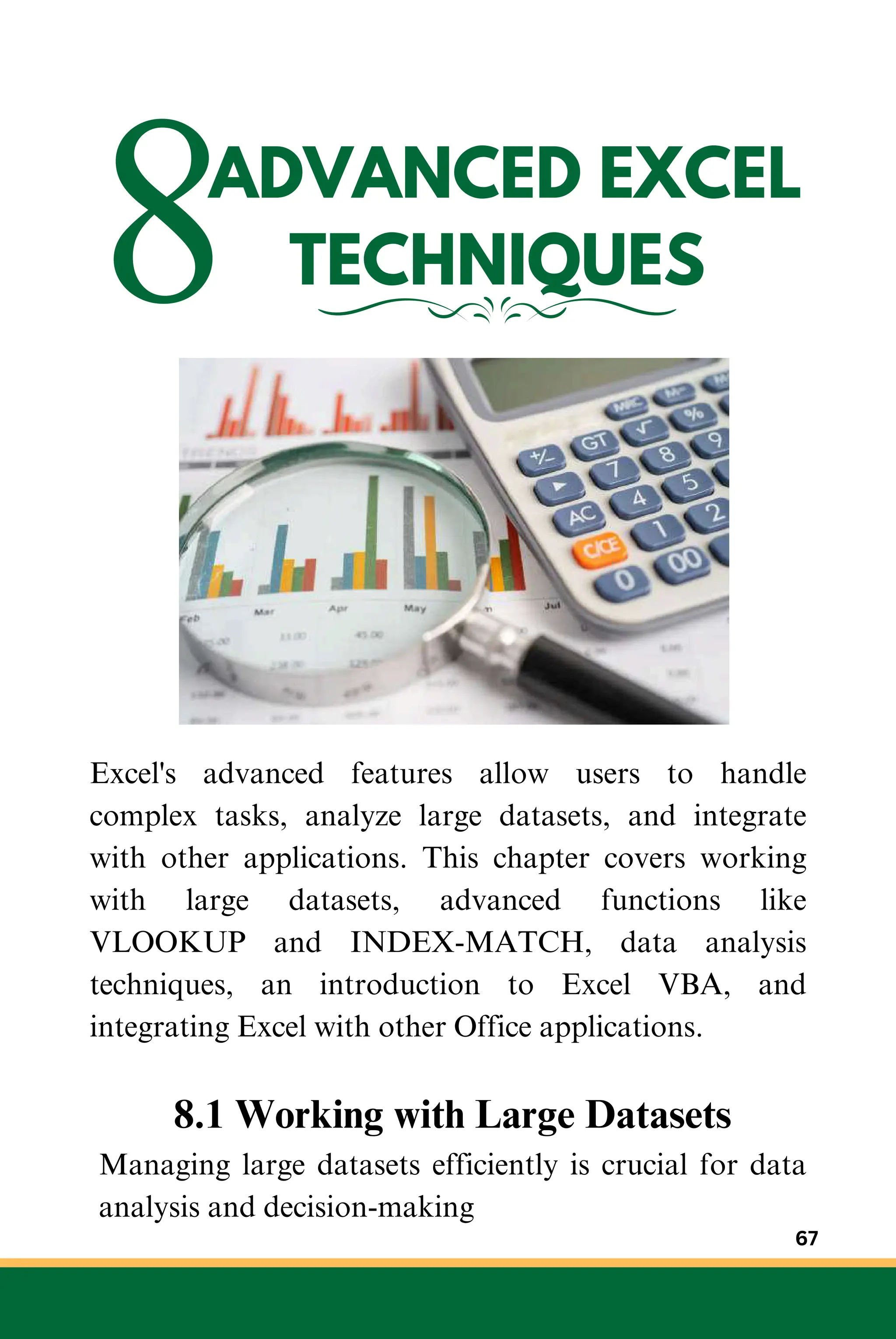


The document is a comprehensive guide to mastering Microsoft Excel, covering essential functions, charts, pivot tables, and practical tips for quick mastery. It includes chapters on navigating the Excel interface, performing basic and advanced calculations, data management, and creating visualizations. The guide aims to equip beginners with foundational knowledge and skills to effectively use Excel in various applications.


