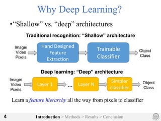
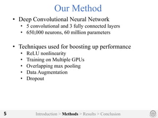
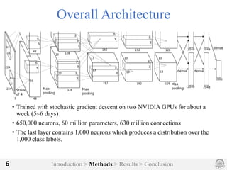
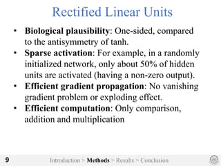
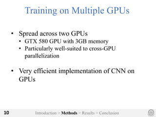
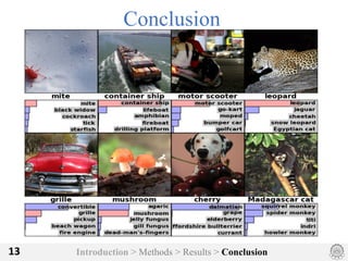
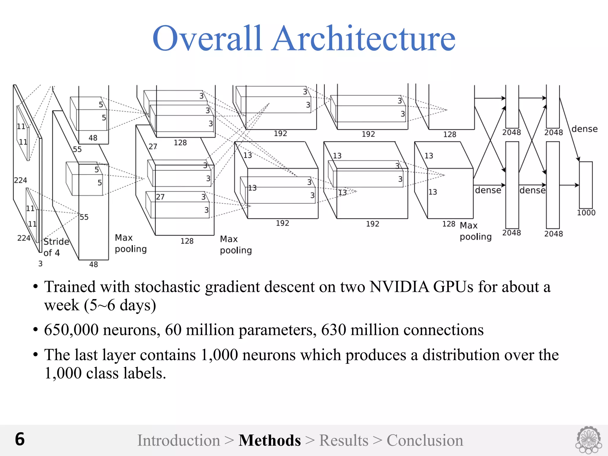
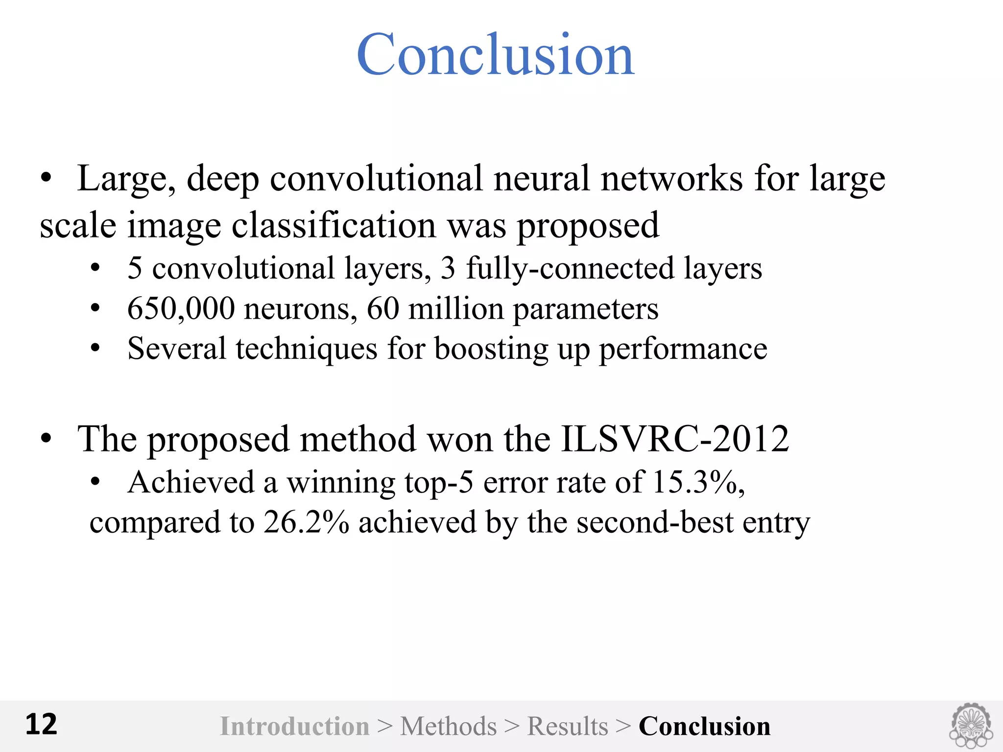
The document discusses an image classification method using deep convolutional neural networks, highlighting its architecture, which includes 5 convolutional and 3 fully connected layers with 650,000 neurons and 60 million parameters. It details the dataset utilized, which consists of over 15 million labeled images from ImageNet and the ILSVRC competition, and describes various performance-boosting techniques such as data augmentation and training on multiple GPUs. The proposed methodology achieved a top-5 error rate of 15.3%, outperforming previous best results in the 2012 competition.
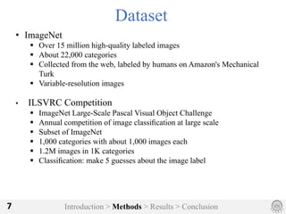
![Model Top-1 Top-5
Sparse coding [3] 47.1% 28.2%
SIFT + FVs [4] 45.7% 25.7%
CNN 37.5 17.0%
Introduction > Methods > Results > Conclusion11
Results & Comparison
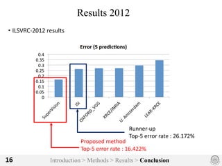
•ILSVRC-2010 test set
ILSVRC-2010 winner
Previous best
published result
Our Method
Comparison of results on ILSRVCs 2010
test set. In italics best results achieved
by others.](https://image.slidesharecdn.com/imageclassificationwithneuralnetworks-191130093901/85/Image-classification-with-neural-networks-11-320.jpg)
![Introduction > Methods > Results > Conclusion14
References
[1] http://cs.nyu.edu/~fergus/tutorials/
deep_learning_cvpr12/fergus_dl_tutorial_final.pptx
[2] reference : http://web.engr.illinois.edu/
~slazebni/spring14/lec24_cnn.pdf
[3] A. Berg, J. Deng, and L. Fei-Fei. Large scale
visual recognition challenge 2010.
www.imagenet.org/challenges. 2010. [4]
S. Tara, Brian Kingsbury, A.-r. Mohamed and
B. Ramabhadran, "Learning Filter Banks within a Deep
[4] J.Sánchezand F.Perronnin.High-dimensional
signature compression for large-scale image classification.
In Computer Vision and Pattern Recognition(CVPR),
2011IEEEConferenceon,pages1665–1672.IEEE, 2011.](https://image.slidesharecdn.com/imageclassificationwithneuralnetworks-191130093901/85/Image-classification-with-neural-networks-14-320.jpg)


![Model Top-1 Top-5
Sparse coding [3] 47.1% 28.2%
SIFT + FVs [4] 45.7% 25.7%
CNN 37.5 17.0%
Introduction > Methods > Results > Conclusion11
Results & Comparison
•ILSVRC-2010 test set
ILSVRC-2010 winner
Previous best
published result
Our Method
Comparison of results on ILSRVCs 2010
test set. In italics best results achieved
by others.](https://image.slidesharecdn.com/imageclassificationwithneuralnetworks-191130093901/75/Image-classification-with-neural-networks-11-2048.jpg)
![Introduction > Methods > Results > Conclusion14
References
[1] http://cs.nyu.edu/~fergus/tutorials/
deep_learning_cvpr12/fergus_dl_tutorial_final.pptx
[2] reference : http://web.engr.illinois.edu/
~slazebni/spring14/lec24_cnn.pdf
[3] A. Berg, J. Deng, and L. Fei-Fei. Large scale
visual recognition challenge 2010.
www.imagenet.org/challenges. 2010. [4]
S. Tara, Brian Kingsbury, A.-r. Mohamed and
B. Ramabhadran, "Learning Filter Banks within a Deep
[4] J.Sánchezand F.Perronnin.High-dimensional
signature compression for large-scale image classification.
In Computer Vision and Pattern Recognition(CVPR),
2011IEEEConferenceon,pages1665–1672.IEEE, 2011.](https://image.slidesharecdn.com/imageclassificationwithneuralnetworks-191130093901/75/Image-classification-with-neural-networks-14-2048.jpg)


![[딥논읽] Meta-Transfer Learning for Zero-Shot Super-Resolution paper review](https://cdn.slidesharecdn.com/ss_thumbnails/210228mzsrv1-210304064113-thumbnail.jpg?width=600ounds&width=560&fit=bounds)


