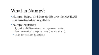
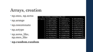
What is Numpy?
•Numpy, Scipy, and Matplotlib provide MATLAB-
like functionality in python.
• Numpy Features:
Typed multidimentional arrays (matrices)
Fast numerical computations (matrix math)
High-level math functions
3.
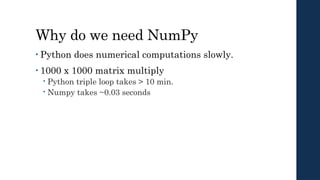
Why do weneed NumPy
• Python does numerical computations slowly.
• 1000 x 1000 matrix multiply
Python triple loop takes > 10 min.
Numpy takes ~0.03 seconds
4.
Logistics: Versioning
• Inthis class, your code will be tested with:
Python 2.7.6
Numpy version: 1.8.2
Scipy version: 0.13.3
OpenCV version: 2.4.8
• Two easy options:
Class virtual machine (always test on the VM)
Anaconda 2 (some assembly required)
5.
NumPy Overview
1. Arrays
2.Shaping and transposition
3. Mathematical Operations
4. Indexing and slicing
5. Broadcasting
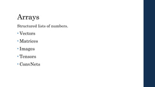
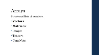
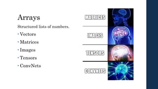
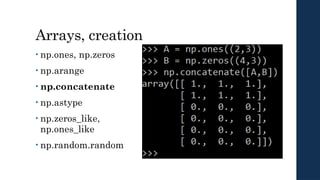
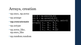
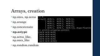
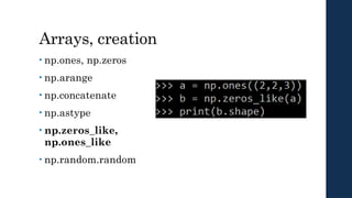
Arrays, Basic Properties
importnumpy as np
a = np.array([[1,2,3],[4,5,6]],dtype=np.float32)
print a.ndim, a.shape, a.dtype
1. Arrays can have any number of dimensions, including zero (a scalar).
2. Arrays are typed: np.uint8, np.int64, np.float32, np.float64
3. Arrays are dense. Each element of the array exists and has the same type.
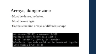
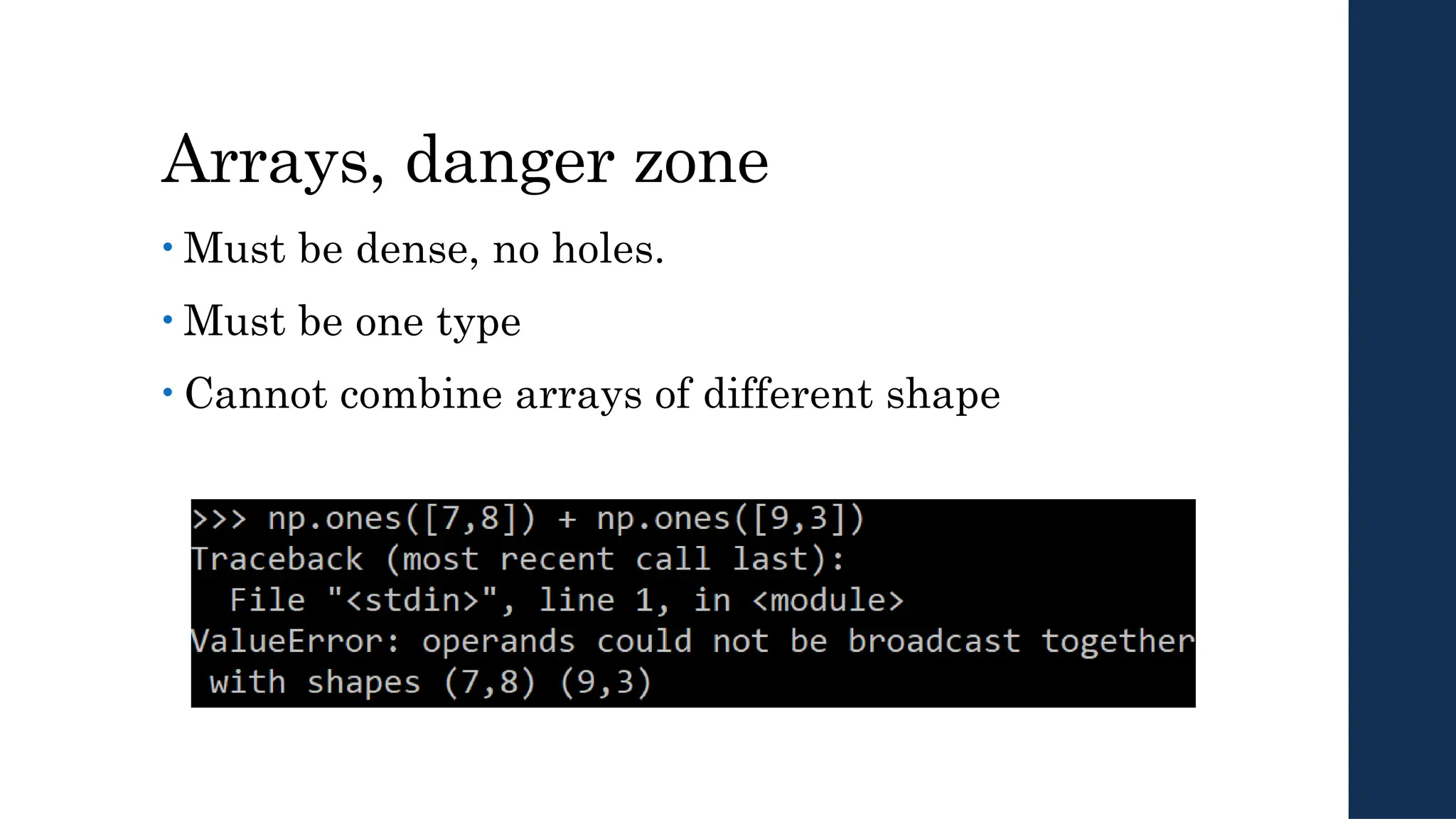
Arrays, danger zone
•Must be dense, no holes.
• Must be one type
• Cannot combine arrays of different shape
21.
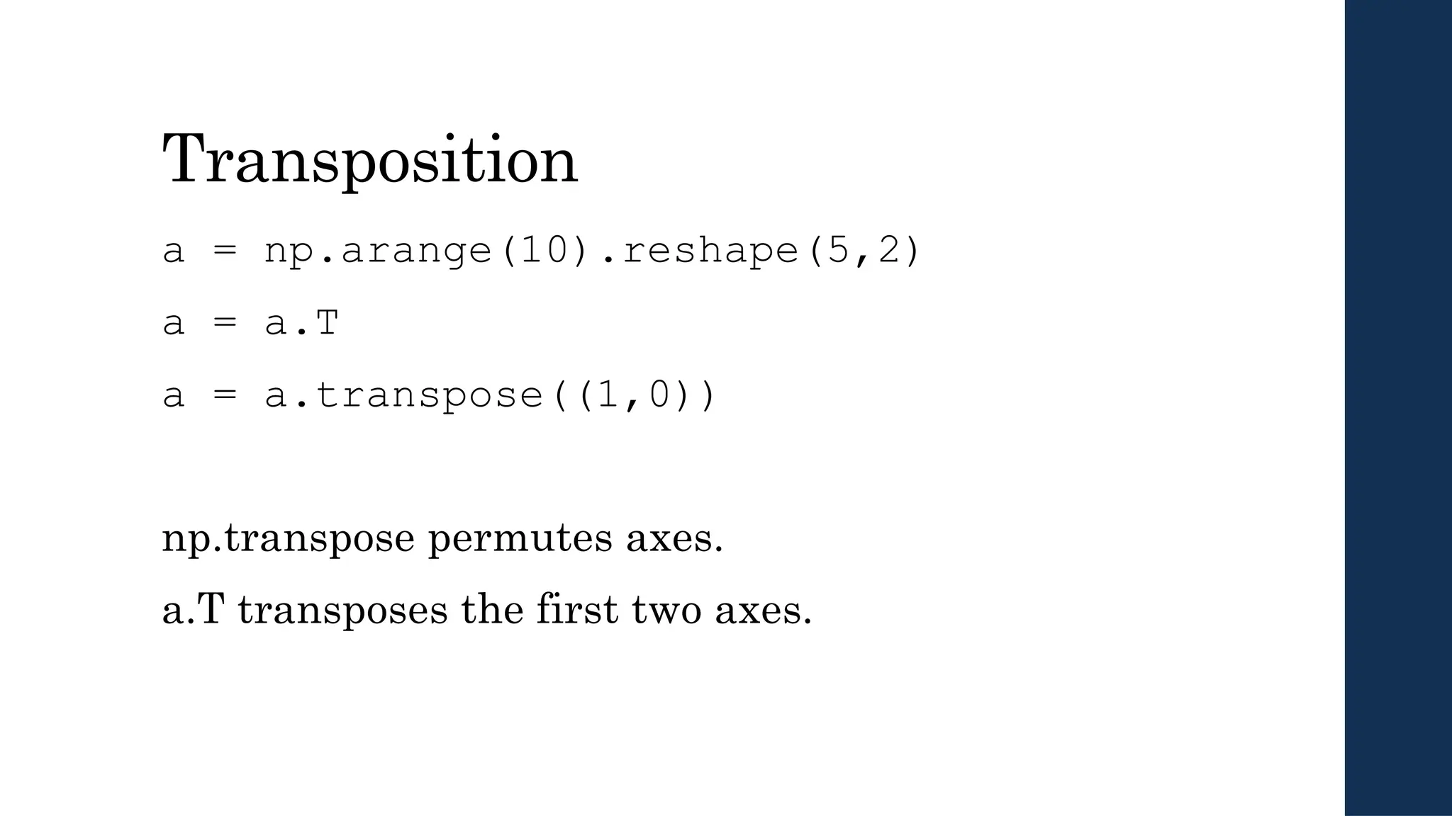
Shaping
a = np.array([1,2,3,4,5,6])
a= a.reshape(3,2)
a = a.reshape(2,-1)
a = a.ravel()
1. Total number of elements cannot change.
2. Use -1 to infer axis shape
3. Row-major by default (MATLAB is column-major)
22.
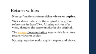
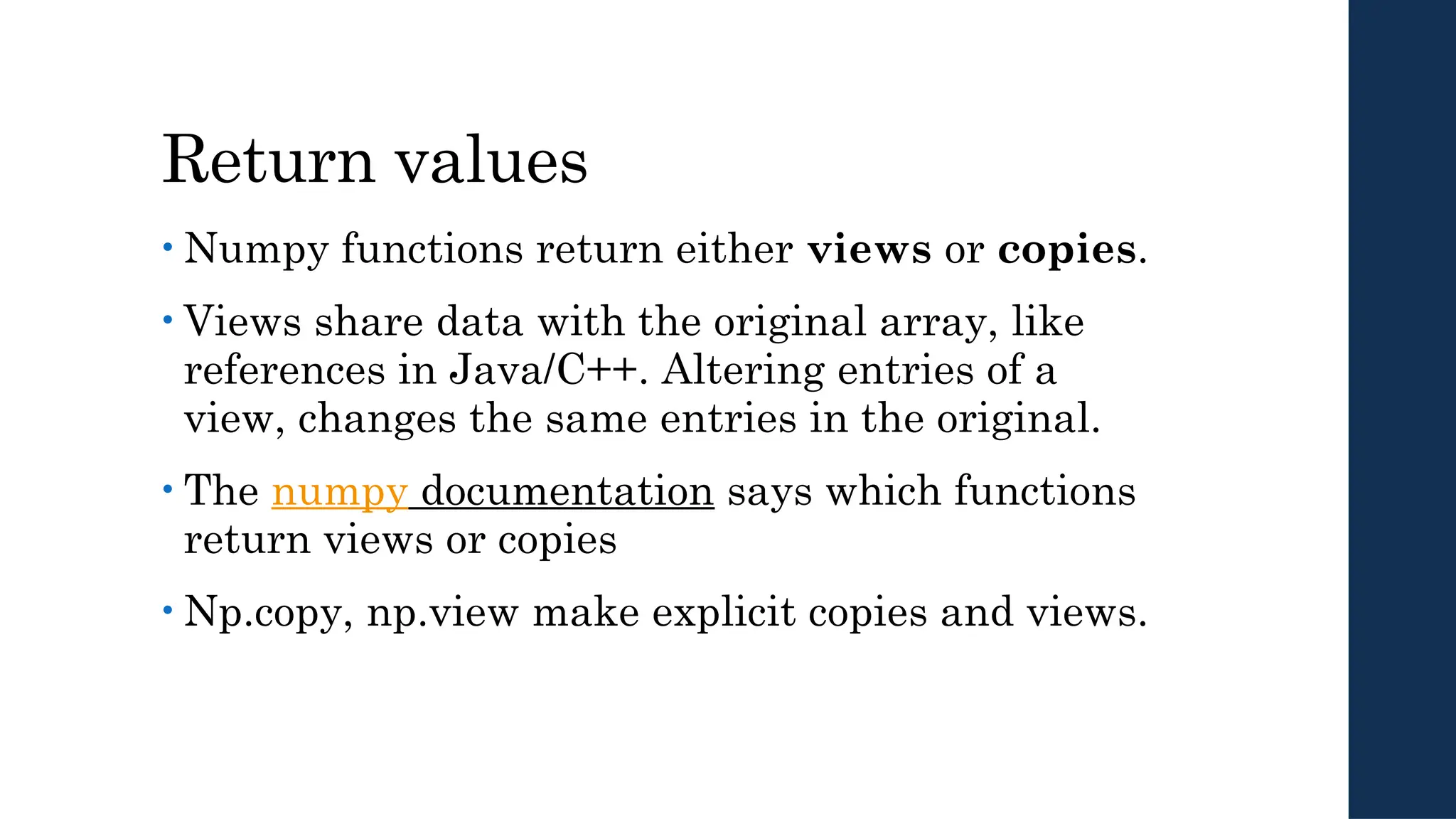
Return values
• Numpyfunctions return either views or copies.
• Views share data with the original array, like
references in Java/C++. Altering entries of a
view, changes the same entries in the original.
• The numpy documentation says which functions
return views or copies
• Np.copy, np.view make explicit copies and views.
Saving and loadingarrays
np.savez(‘data.npz’, a=a)
data = np.load(‘data.npz’)
a = data[‘a’]
1. NPZ files can hold multiple arrays
2. np.savez_compressed similar.
25.
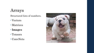
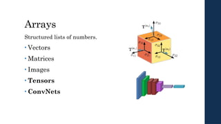
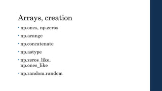
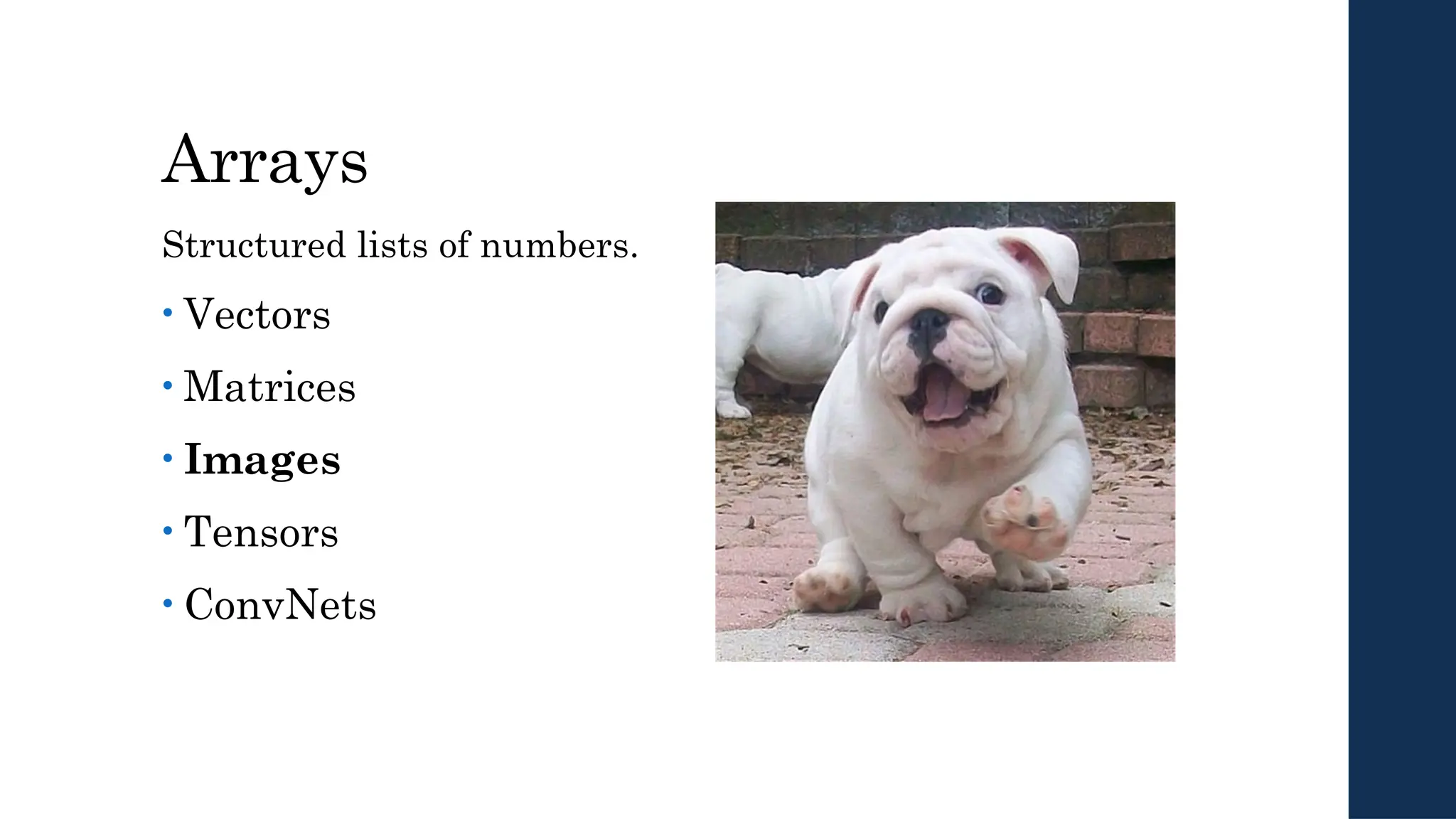
Image arrays
Images are3D arrays: width, height, and channels
Common image formats:
height x width x RGB (band-interleaved)
height x width (band-sequential)
Gotchas:
Channels may also be BGR (OpenCV does this)
May be [width x height], not [height x width]
26.
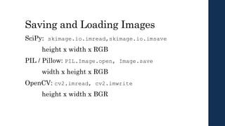
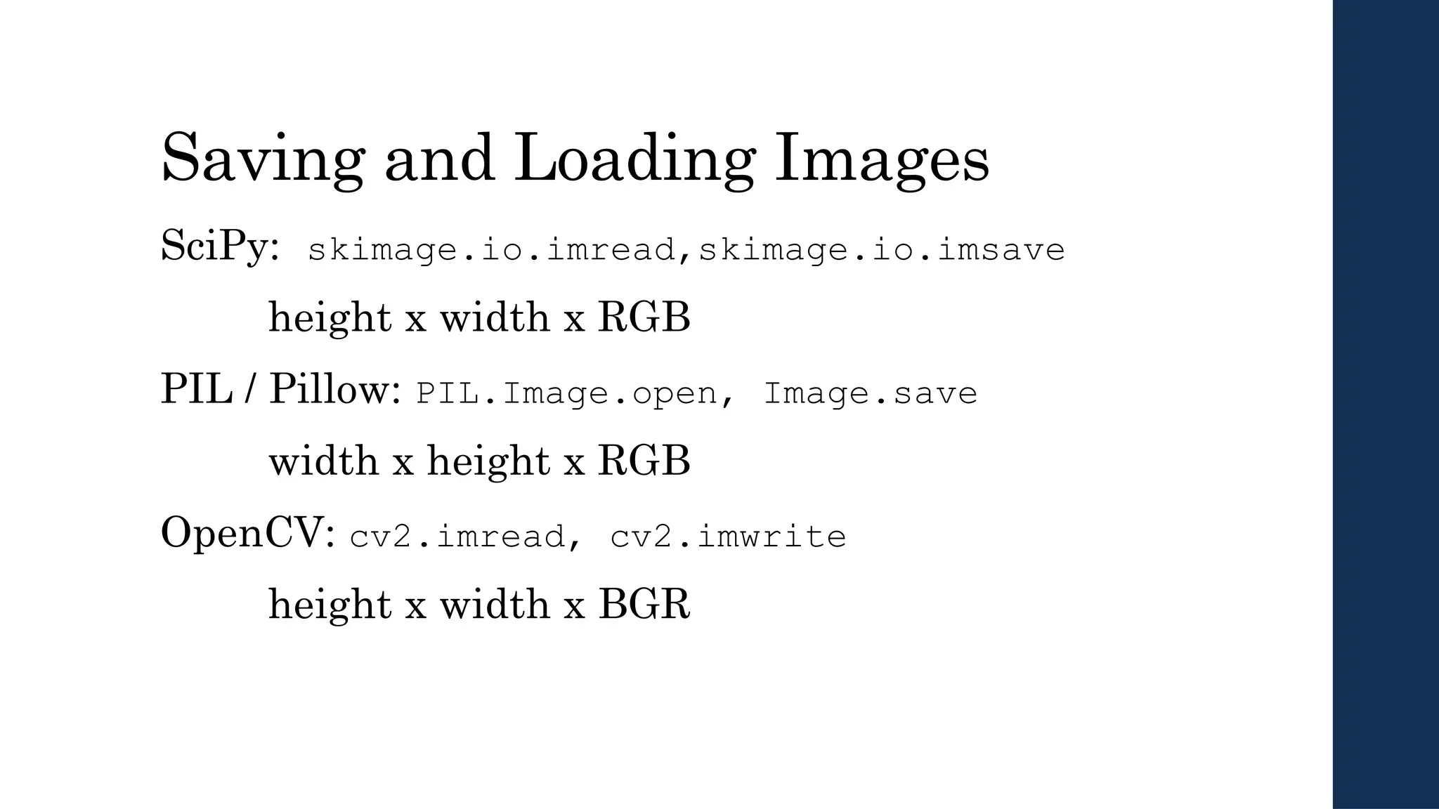
Saving and LoadingImages
SciPy: skimage.io.imread,skimage.io.imsave
height x width x RGB
PIL / Pillow: PIL.Image.open, Image.save
width x height x RGB
OpenCV: cv2.imread, cv2.imwrite
height x width x BGR
27.
Recap
We just sawhow to create arrays, reshape them,
and permute axes
Questions so far?
28.
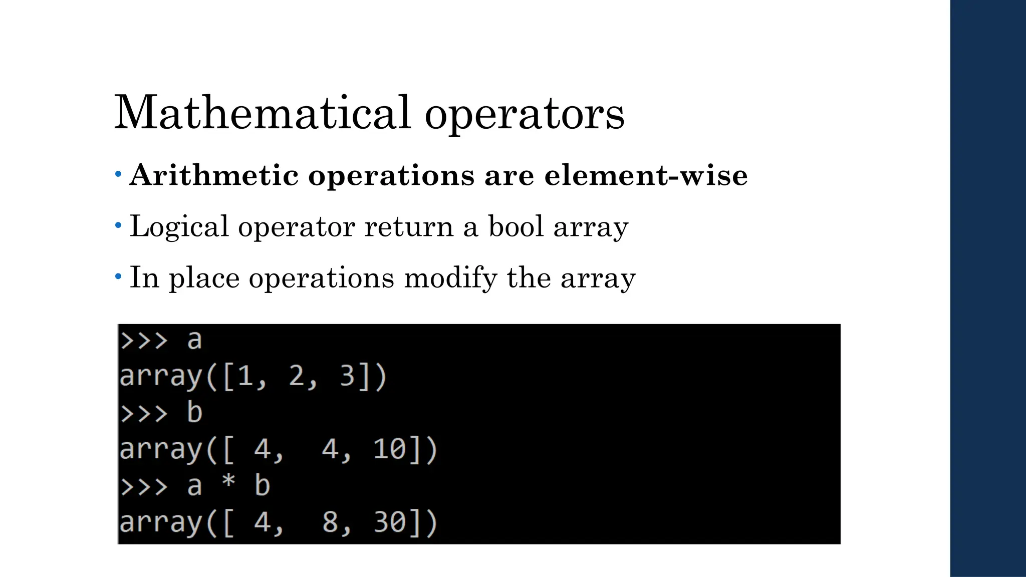
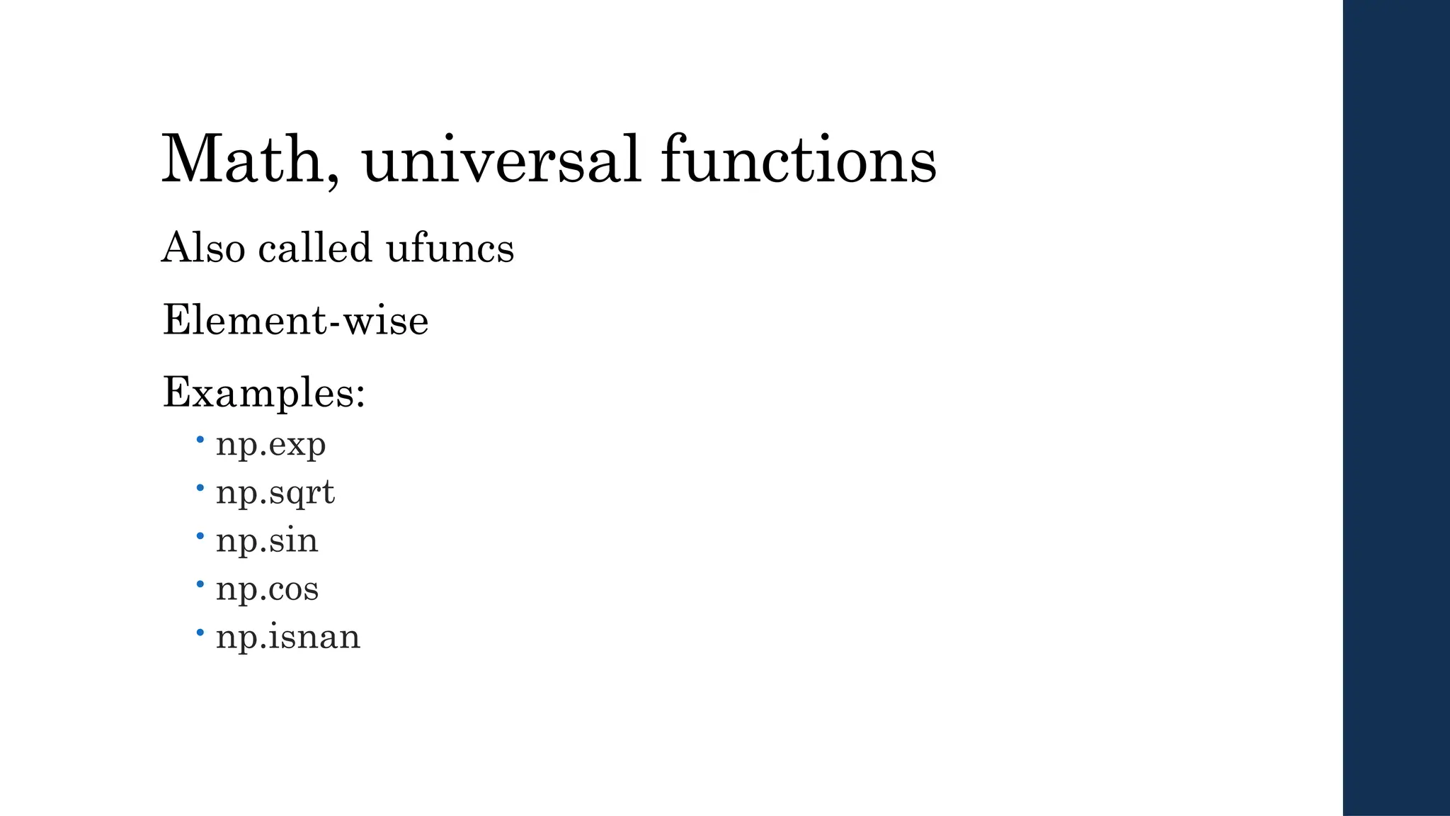
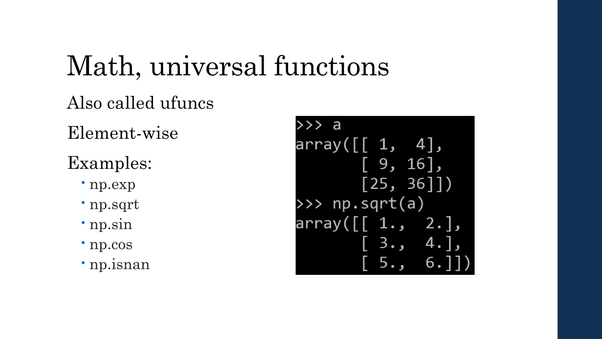
Mathematical operators
• Arithmeticoperations are element-wise
• Logical operator return a bool array
• In place operations modify the array
29.
Mathematical operators
• Arithmeticoperations are element-wise
• Logical operator return a bool array
• In place operations modify the array
30.
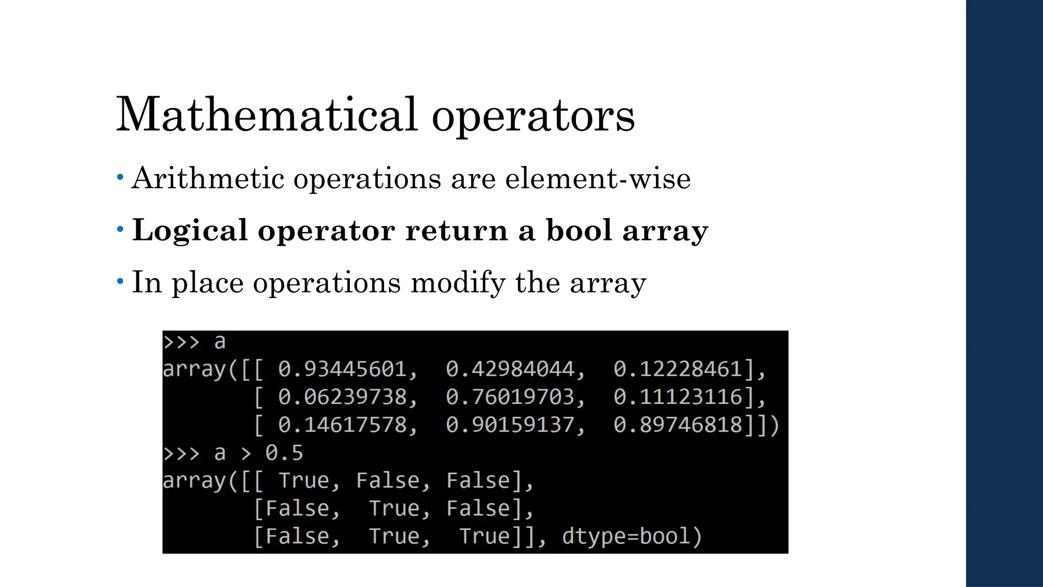
Mathematical operators
• Arithmeticoperations are element-wise
• Logical operator return a bool array
• In place operations modify the array
31.
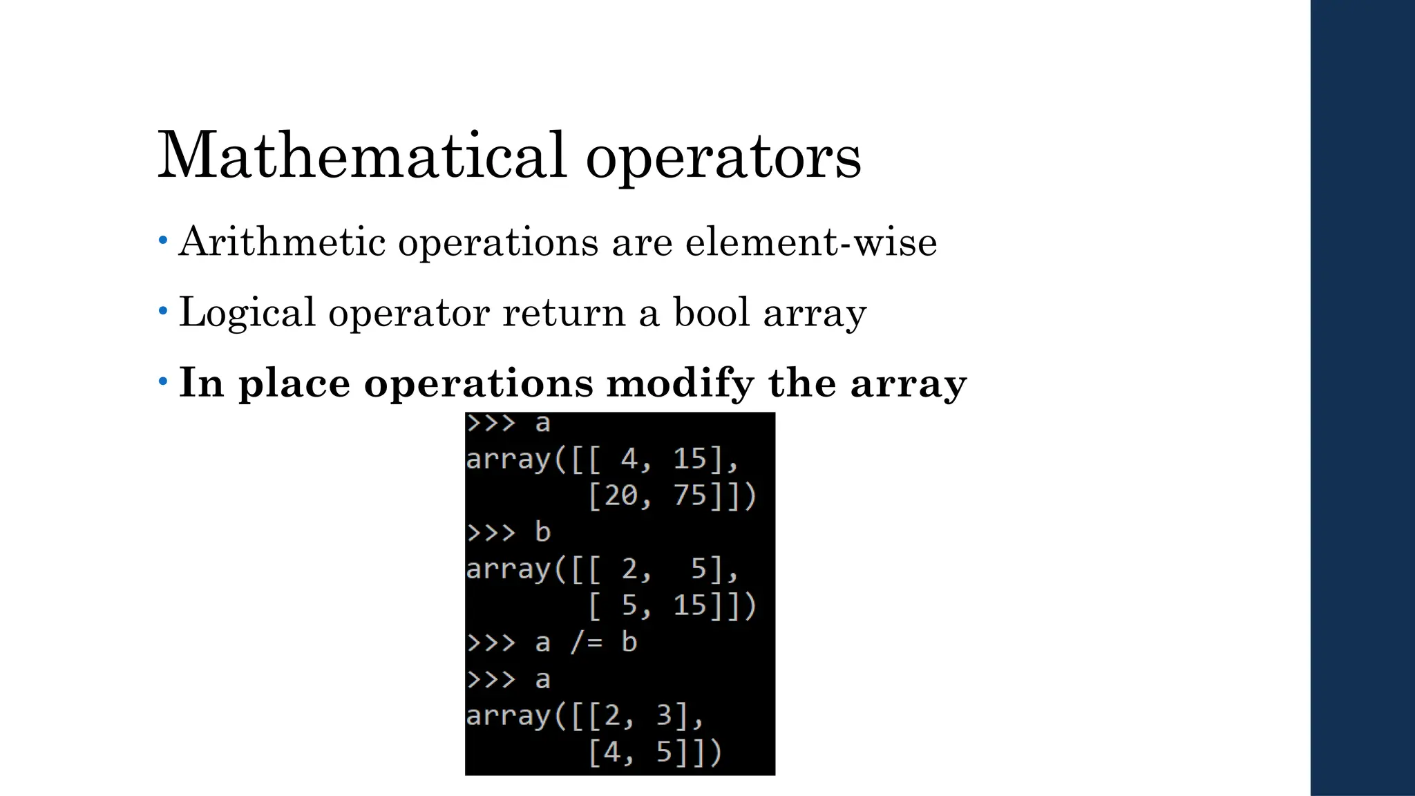
Mathematical operators
• Arithmeticoperations are element-wise
• Logical operator return a bool array
• In place operations modify the array
32.
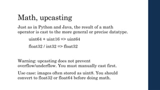
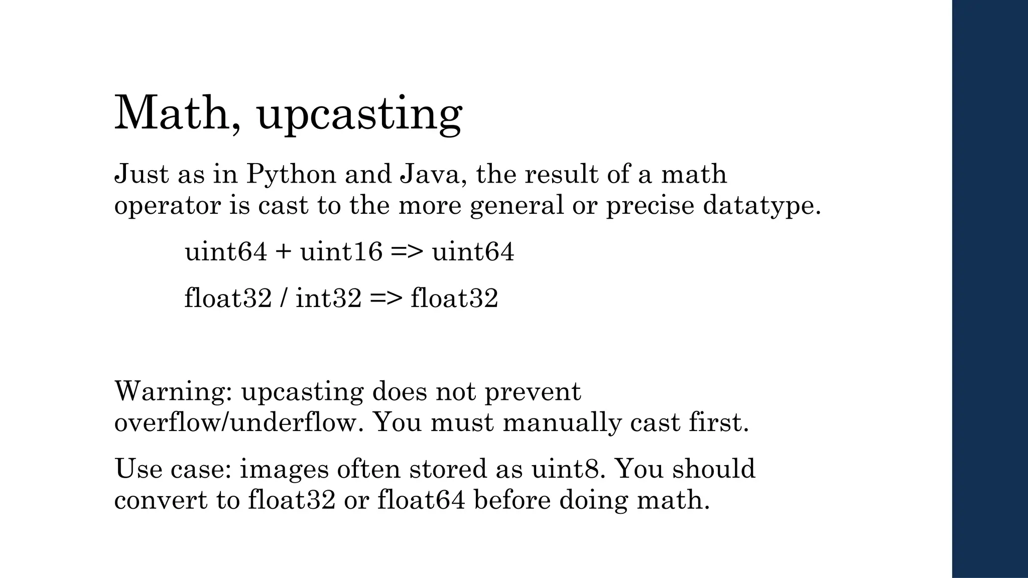
Math, upcasting
Just asin Python and Java, the result of a math
operator is cast to the more general or precise datatype.
uint64 + uint16 => uint64
float32 / int32 => float32
Warning: upcasting does not prevent
overflow/underflow. You must manually cast first.
Use case: images often stored as uint8. You should
convert to float32 or float64 before doing math.
Indexing
x[0,0] # top-leftelement
x[0,-1] # first row, last column
x[0,:] # first row (many entries)
x[:,0] # first column (many entries)
Notes:
Zero-indexing
Multi-dimensional indices are comma-separated (i.e., a
tuple)
37.
Indexing, slices andarrays
I[1:-1,1:-1] # select all but one-pixel border
I = I[:,:,::-1] # swap channel order
I[I<10] = 0 # set dark pixels to black
I[[1,3], :] # select 2nd and 4th row
1. Slices are views. Writing to a slice overwrites the
original array.
2. Can also index by a list or boolean array.
38.
Python Slicing
Syntax: start:stop:step
a= list(range(10))
a[:3] # indices 0, 1, 2
a[-3:] # indices 7, 8, 9
a[3:8:2] # indices 3, 5, 7
a[4:1:-1] # indices 4, 3, 2 (this one is tricky)
39.
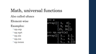
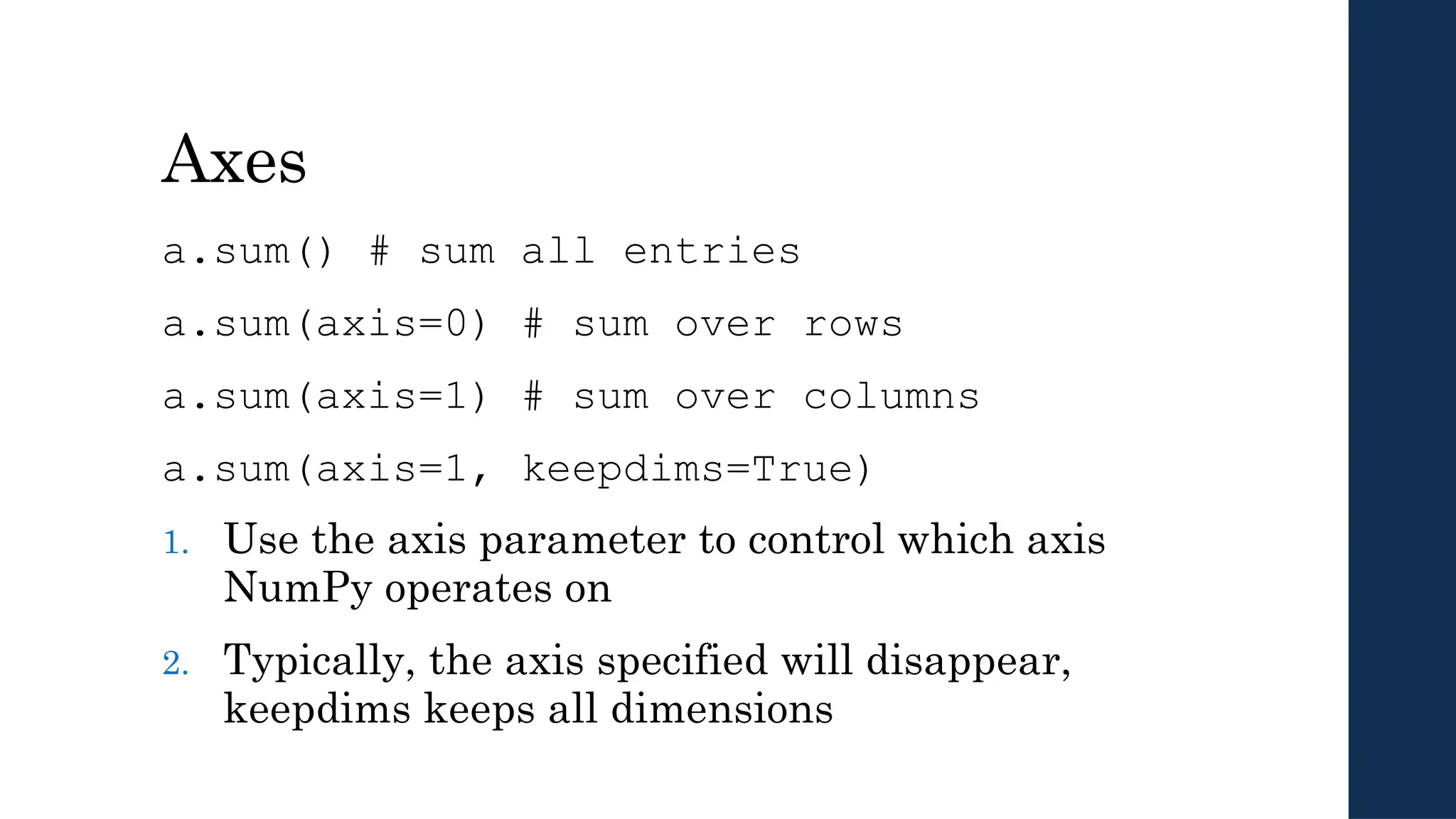
Axes
a.sum() # sumall entries
a.sum(axis=0) # sum over rows
a.sum(axis=1) # sum over columns
a.sum(axis=1, keepdims=True)
1. Use the axis parameter to control which axis
NumPy operates on
2. Typically, the axis specified will disappear,
keepdims keeps all dimensions
40.
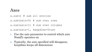
Broadcasting
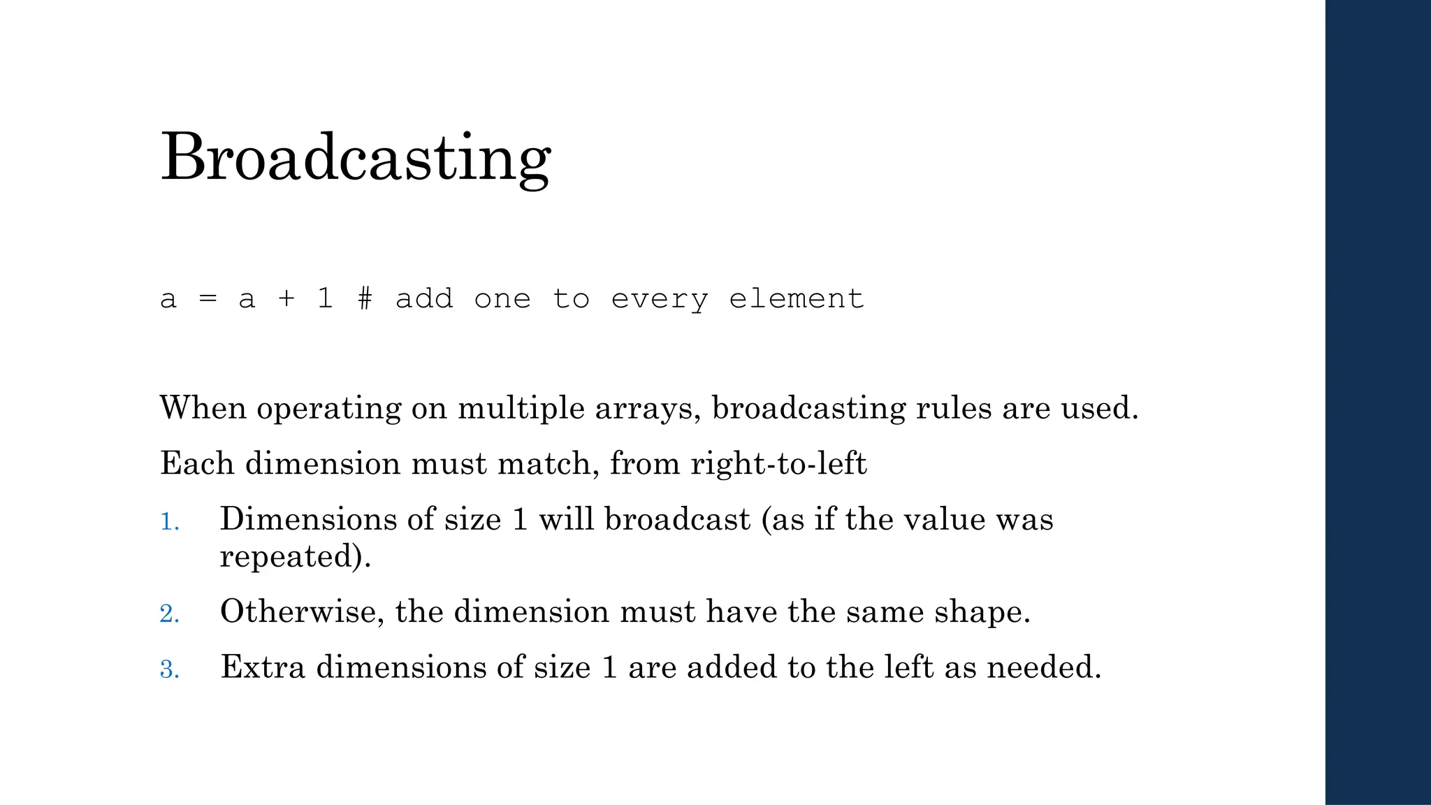
a = a+ 1 # add one to every element
When operating on multiple arrays, broadcasting rules are used.
Each dimension must match, from right-to-left
1. Dimensions of size 1 will broadcast (as if the value was
repeated).
2. Otherwise, the dimension must have the same shape.
3. Extra dimensions of size 1 are added to the left as needed.
41.
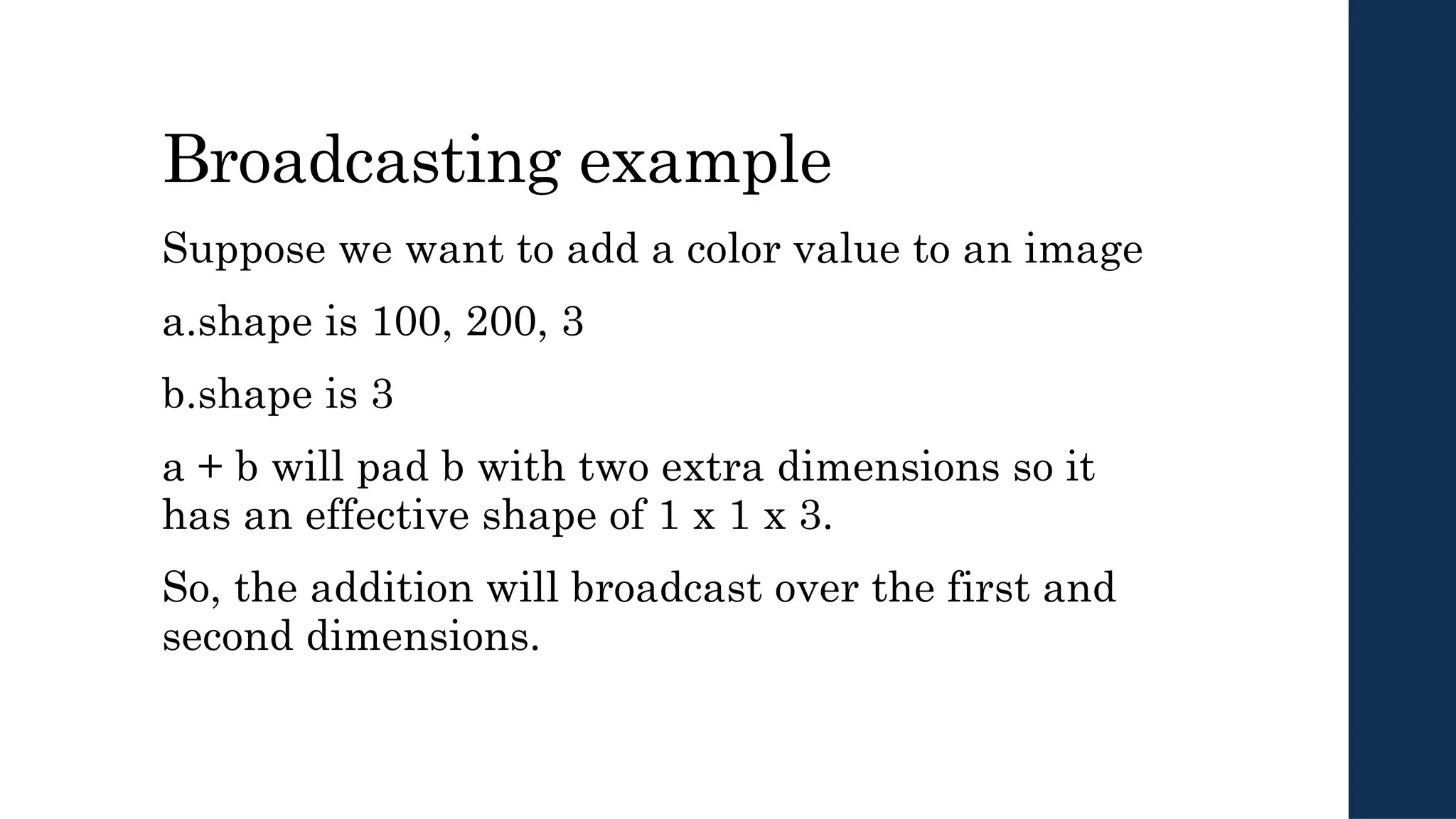
Broadcasting example
Suppose wewant to add a color value to an image
a.shape is 100, 200, 3
b.shape is 3
a + b will pad b with two extra dimensions so it
has an effective shape of 1 x 1 x 3.
So, the addition will broadcast over the first and
second dimensions.
42.
Broadcasting failures
If a.shapeis 100, 200, 3 but b.shape is 4 then a + b
will fail. The trailing dimensions must have the
same shape (or be 1)
43.
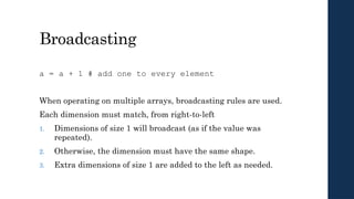
Tips to avoidbugs
1. Know what your datatypes are.
2. Check whether you have a view or a copy.
3. Use matplotlib for sanity checks.
4. Use pdb to check each step of your computation.
5. Know np.dot vs np.mult.

![Arrays, Basic Properties
import numpy as np
a = np.array([[1,2,3],[4,5,6]],dtype=np.float32)
print a.ndim, a.shape, a.dtype
1. Arrays can have any number of dimensions, including zero (a scalar).
2. Arrays are typed: np.uint8, np.int64, np.float32, np.float64
3. Arrays are dense. Each element of the array exists and has the same type.](https://image.slidesharecdn.com/numpyinpython-250924085926-6a5e1a79/85/Introduction-to-Numpy-module-in-Python-pptx-11-320.jpg)
![Shaping
a = np.array([1,2,3,4,5,6])
a = a.reshape(3,2)
a = a.reshape(2,-1)
a = a.ravel()
1. Total number of elements cannot change.
2. Use -1 to infer axis shape
3. Row-major by default (MATLAB is column-major)](https://image.slidesharecdn.com/numpyinpython-250924085926-6a5e1a79/85/Introduction-to-Numpy-module-in-Python-pptx-21-320.jpg)

![Saving and loading arrays
np.savez(‘data.npz’, a=a)
data = np.load(‘data.npz’)
a = data[‘a’]
1. NPZ files can hold multiple arrays
2. np.savez_compressed similar.](https://image.slidesharecdn.com/numpyinpython-250924085926-6a5e1a79/85/Introduction-to-Numpy-module-in-Python-pptx-24-320.jpg)
![Image arrays
Images are 3D arrays: width, height, and channels
Common image formats:
height x width x RGB (band-interleaved)
height x width (band-sequential)
Gotchas:
Channels may also be BGR (OpenCV does this)
May be [width x height], not [height x width]](https://image.slidesharecdn.com/numpyinpython-250924085926-6a5e1a79/85/Introduction-to-Numpy-module-in-Python-pptx-25-320.jpg)


![Indexing
x[0,0] # top-left element
x[0,-1] # first row, last column
x[0,:] # first row (many entries)
x[:,0] # first column (many entries)
Notes:
Zero-indexing
Multi-dimensional indices are comma-separated (i.e., a
tuple)](https://image.slidesharecdn.com/numpyinpython-250924085926-6a5e1a79/85/Introduction-to-Numpy-module-in-Python-pptx-36-320.jpg)
![Indexing, slices and arrays
I[1:-1,1:-1] # select all but one-pixel border
I = I[:,:,::-1] # swap channel order
I[I<10] = 0 # set dark pixels to black
I[[1,3], :] # select 2nd and 4th row
1. Slices are views. Writing to a slice overwrites the
original array.
2. Can also index by a list or boolean array.](https://image.slidesharecdn.com/numpyinpython-250924085926-6a5e1a79/85/Introduction-to-Numpy-module-in-Python-pptx-37-320.jpg)
![Python Slicing
Syntax: start:stop:step
a = list(range(10))
a[:3] # indices 0, 1, 2
a[-3:] # indices 7, 8, 9
a[3:8:2] # indices 3, 5, 7
a[4:1:-1] # indices 4, 3, 2 (this one is tricky)](https://image.slidesharecdn.com/numpyinpython-250924085926-6a5e1a79/85/Introduction-to-Numpy-module-in-Python-pptx-38-320.jpg)


![Arrays, Basic Properties
import numpy as np
a = np.array([[1,2,3],[4,5,6]],dtype=np.float32)
print a.ndim, a.shape, a.dtype
1. Arrays can have any number of dimensions, including zero (a scalar).
2. Arrays are typed: np.uint8, np.int64, np.float32, np.float64
3. Arrays are dense. Each element of the array exists and has the same type.](https://image.slidesharecdn.com/numpyinpython-250924085926-6a5e1a79/75/Introduction-to-Numpy-module-in-Python-pptx-11-2048.jpg)
![Shaping
a = np.array([1,2,3,4,5,6])
a = a.reshape(3,2)
a = a.reshape(2,-1)
a = a.ravel()
1. Total number of elements cannot change.
2. Use -1 to infer axis shape
3. Row-major by default (MATLAB is column-major)](https://image.slidesharecdn.com/numpyinpython-250924085926-6a5e1a79/75/Introduction-to-Numpy-module-in-Python-pptx-21-2048.jpg)
![Saving and loading arrays
np.savez(‘data.npz’, a=a)
data = np.load(‘data.npz’)
a = data[‘a’]
1. NPZ files can hold multiple arrays
2. np.savez_compressed similar.](https://image.slidesharecdn.com/numpyinpython-250924085926-6a5e1a79/75/Introduction-to-Numpy-module-in-Python-pptx-24-2048.jpg)
![Image arrays
Images are 3D arrays: width, height, and channels
Common image formats:
height x width x RGB (band-interleaved)
height x width (band-sequential)
Gotchas:
Channels may also be BGR (OpenCV does this)
May be [width x height], not [height x width]](https://image.slidesharecdn.com/numpyinpython-250924085926-6a5e1a79/75/Introduction-to-Numpy-module-in-Python-pptx-25-2048.jpg)

![Indexing
x[0,0] # top-left element
x[0,-1] # first row, last column
x[0,:] # first row (many entries)
x[:,0] # first column (many entries)
Notes:
Zero-indexing
Multi-dimensional indices are comma-separated (i.e., a
tuple)](https://image.slidesharecdn.com/numpyinpython-250924085926-6a5e1a79/75/Introduction-to-Numpy-module-in-Python-pptx-36-2048.jpg)
![Indexing, slices and arrays
I[1:-1,1:-1] # select all but one-pixel border
I = I[:,:,::-1] # swap channel order
I[I<10] = 0 # set dark pixels to black
I[[1,3], :] # select 2nd and 4th row
1. Slices are views. Writing to a slice overwrites the
original array.
2. Can also index by a list or boolean array.](https://image.slidesharecdn.com/numpyinpython-250924085926-6a5e1a79/75/Introduction-to-Numpy-module-in-Python-pptx-37-2048.jpg)
![Python Slicing
Syntax: start:stop:step
a = list(range(10))
a[:3] # indices 0, 1, 2
a[-3:] # indices 7, 8, 9
a[3:8:2] # indices 3, 5, 7
a[4:1:-1] # indices 4, 3, 2 (this one is tricky)](https://image.slidesharecdn.com/numpyinpython-250924085926-6a5e1a79/75/Introduction-to-Numpy-module-in-Python-pptx-38-2048.jpg)


![NUMPY [Autosaved] .pptx](https://cdn.slidesharecdn.com/ss_thumbnails/numpyautosaved-240106041504-989a0cc3-thumbnail.jpg?width=600ounds&width=560&fit=bounds)


