The document outlines key concepts in data mining, including supervised learning techniques like classification and prediction, as well as unsupervised learning methods such as clustering and association rules. It details the steps involved in the data mining process, from defining the purpose and obtaining data to model assessment and deployment. Additionally, it highlights data splitting techniques to ensure unbiased model performance assessment.

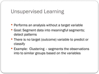

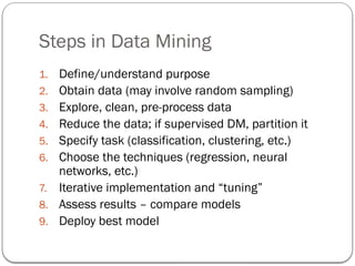
![Data Splitting
Data are split into training and test sets.
Training data is used to train the model
Testing data is used to estimate an unbiased assessment of the
model’s performance
#Random splitting of iris data into 70% train and 30%test datasets
ind <- sample(2, nrow(data), replace=TRUE, prob=c(0.7, 0.3))
trainData <- data[ind==1,]
testData <- data[ind==2,]](https://image.slidesharecdn.com/introtodatamining1-240821175312-0e735051/85/IntroToDataMining-Key-Components-and-process-14-320.jpg)
![Simple Random Sampling
All observations have an equal chance of selection
# Using base R
set.seed(123) # for reproducibility
index_1 <- sample(1:nrow(ames), round(nrow(ames) * 0.7))
train_1 <- ames[index_1, ]
test_1 <- ames[-index_1, ]](https://image.slidesharecdn.com/introtodatamining1-240821175312-0e735051/85/IntroToDataMining-Key-Components-and-process-15-320.jpg)


![Data Splitting
Data are split into training and test sets.
Training data is used to train the model
Testing data is used to estimate an unbiased assessment of the
model’s performance
#Random splitting of iris data into 70% train and 30%test datasets
ind <- sample(2, nrow(data), replace=TRUE, prob=c(0.7, 0.3))
trainData <- data[ind==1,]
testData <- data[ind==2,]](https://image.slidesharecdn.com/introtodatamining1-240821175312-0e735051/75/IntroToDataMining-Key-Components-and-process-14-2048.jpg)
![Simple Random Sampling
All observations have an equal chance of selection
# Using base R
set.seed(123) # for reproducibility
index_1 <- sample(1:nrow(ames), round(nrow(ames) * 0.7))
train_1 <- ames[index_1, ]
test_1 <- ames[-index_1, ]](https://image.slidesharecdn.com/introtodatamining1-240821175312-0e735051/75/IntroToDataMining-Key-Components-and-process-15-2048.jpg)


![Agentic Systems and Compliance - A brief intro [1.2]](https://cdn.slidesharecdn.com/ss_thumbnails/agenticsystemsandcompliace-1-251018025303-958a42ec-thumbnail.jpg?width=600ounds&width=560&fit=bounds)


![Matrix and determinant URT [Autosaved].pptx](https://cdn.slidesharecdn.com/ss_thumbnails/matrixanddeterminanturtautosaved-251018190340-9e6a6deb-thumbnail.jpg?width=600ounds&width=560&fit=bounds)


