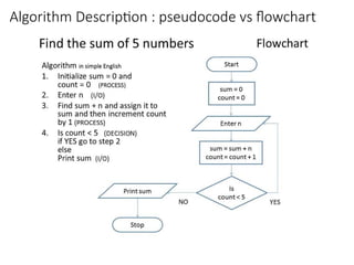
Algorithm
In simple terms,an algorithm is a series of instructions to
solve a problem (complete a task)
Problems can be in any form
Business/Academia
How to maximize profit under certain constrains? (Linear programming)
Maximize the number of classes running in parallel
Life
Explain how to compute GCD to a 8 year old child
Explain how to tie a tie
• We are often unaware that we are using algorithms in real life
• In CS we must be super-aware of the details of algorithms we need
- because we need to translate these algorithms to computer so that it can work for us
3.
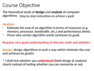
Course Objective
The theoreticalstudy of design and analysis of computer
algorithms
Analysis:
• Estimate the cost of an algorithm in terms of resources (e.g.
memory, processor, bandwidth, etc.) and performance (time).
• Prove why certain algorithm works (achieves its goal).
Requires very good understanding of discrete math and statistics
Design: design algorithms in such a way which minimize the cost
and achieves its goal(s)
* I shall test whether you understood (both design & analysis)
clearly instead of testing whether you can memorize or not.
(step by step instructions to achieve a goal)
4.
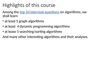
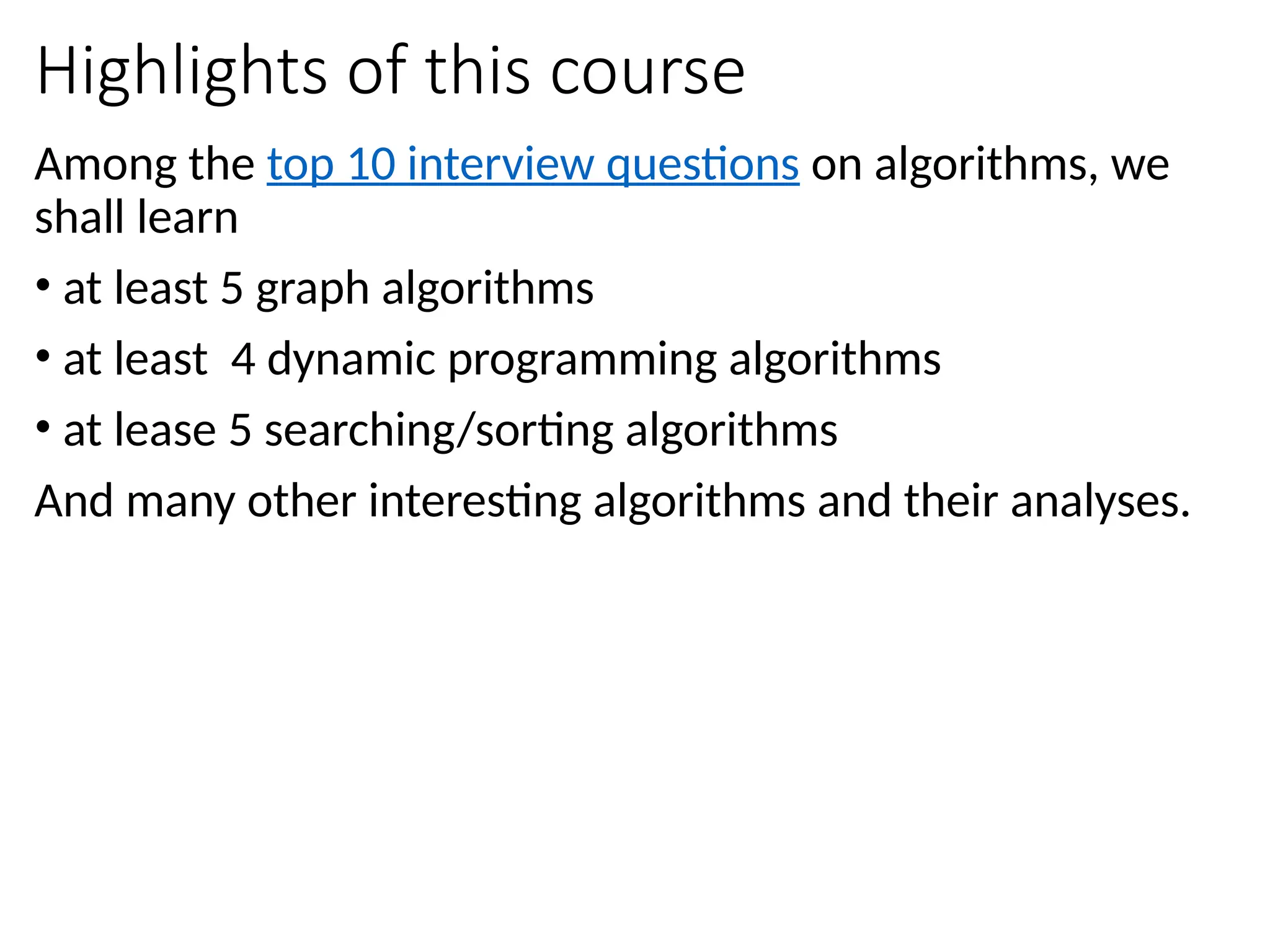
Highlights of thiscourse
Among the top 10 interview questions on algorithms, we
shall learn
• at least 5 graph algorithms
• at least 4 dynamic programming algorithms
• at lease 5 searching/sorting algorithms
And many other interesting algorithms and their analyses.
5.
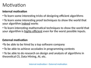
Motivation
Internal motivation
• Tolearn some interesting tricks of designing efficient algorithms
• To learn some interesting proof techniques to show the world that
your algorithm indeed works
• To learn interesting mathematical techniques to show the world that
your algorithm is highly efficient even for the worst possible inputs.
External motivation
•To be able to be hired by a top software company
• To be able to achieve accolades in programming contests
• To be able to do research on design and analysis of algorithms in
theoretical CS, Data Mining, AI, etc.
Internal motivation > External motivation
6.
Computational Problem
A computationalproblem can be represented as a question
that describes the requirements of the desired output given
an input. For e.g.
• Is n a prime number? (n is a user input)
• What are the prime factors of n? (n is a user input)
• How many prime factors of n are there? (n is user input)
• What is the maximum value of a[i]? (a[1…n] is an input
array)
7.
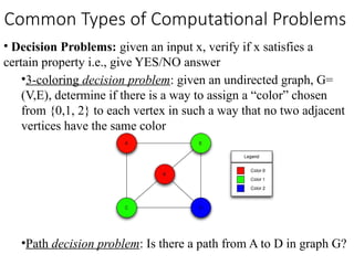
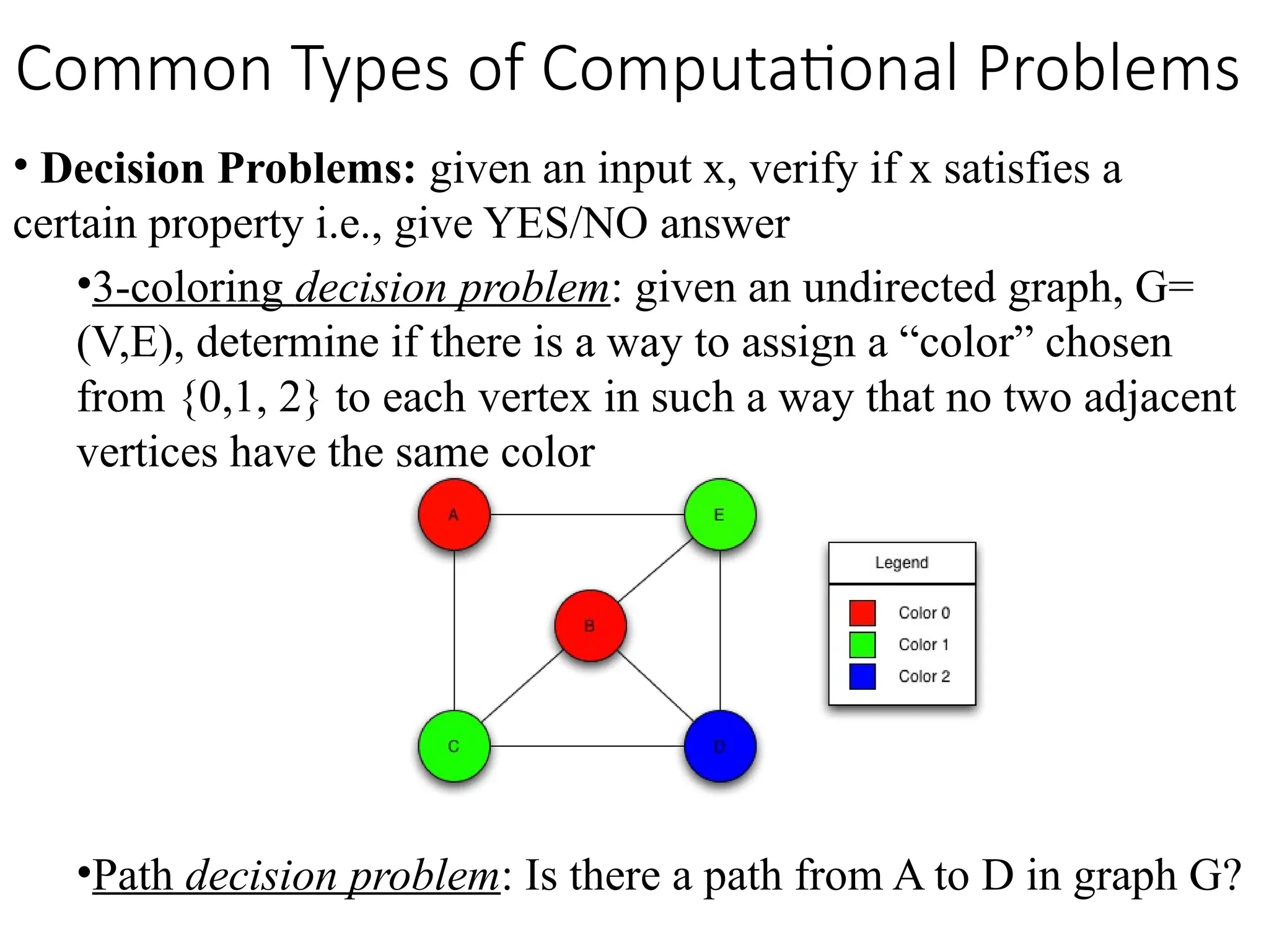
• Decision Problems:given an input x, verify if x satisfies a
certain property i.e., give YES/NO answer
•3-coloring decision problem: given an undirected graph, G=
(V,E), determine if there is a way to assign a “color” chosen
from {0,1, 2} to each vertex in such a way that no two adjacent
vertices have the same color
•Path decision problem: Is there a path from A to D in graph G?
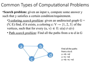
Common Types of Computational Problems
8.
•Search problem: givenan input x, compute some answer y
such that y satisfies a certain condition/requirement.
•3-coloring search problem: given an undirected graph G =
(V, E) find, if it exists, a coloring c: V → {1, 2, 3} of the
vertices, such that for every (u, v) E: c(u) ≠ c(v)
∈
• Path search problem: Find all the paths from a to d in G
a b
c
d
Find all the paths
from a to d:
a →b →d
a →c →d
a →b →c →d
Common Types of Computational Problems
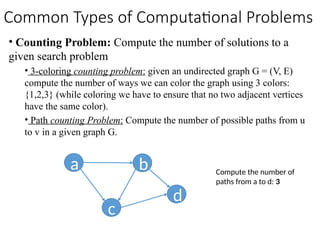
9.
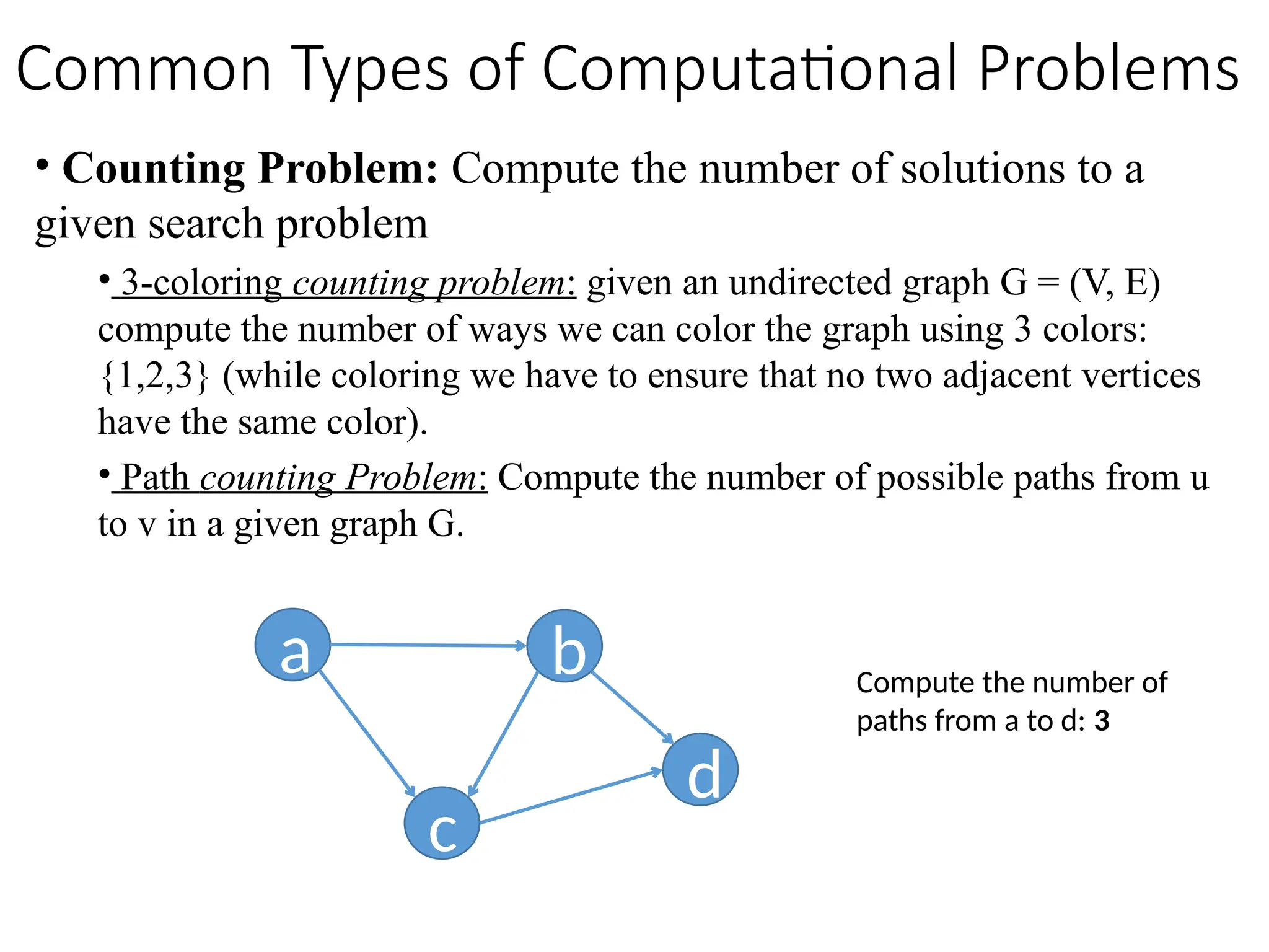
• Counting Problem:Compute the number of solutions to a
given search problem
• 3-coloring counting problem: given an undirected graph G = (V, E)
compute the number of ways we can color the graph using 3 colors:
{1,2,3} (while coloring we have to ensure that no two adjacent vertices
have the same color).
• Path counting Problem: Compute the number of possible paths from u
to v in a given graph G.
a b
c
d
Compute the number of
paths from a to d: 3
Common Types of Computational Problems
10.
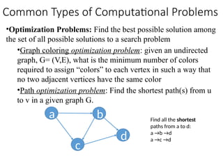
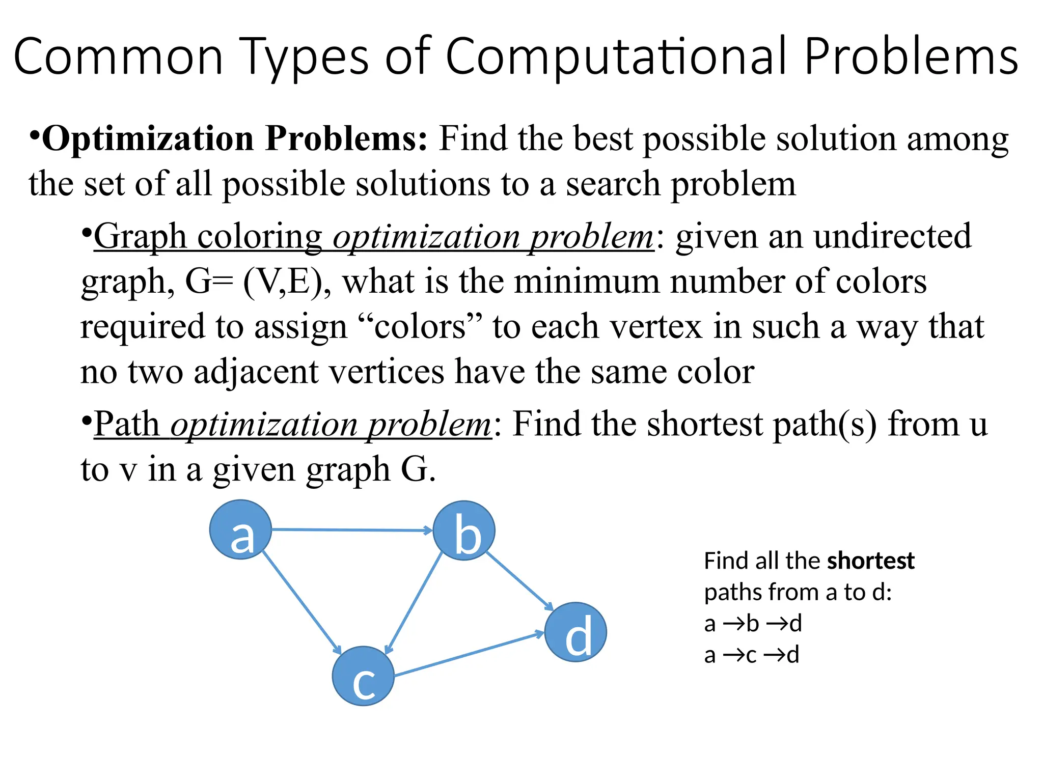
•Optimization Problems: Findthe best possible solution among
the set of all possible solutions to a search problem
•Graph coloring optimization problem: given an undirected
graph, G= (V,E), what is the minimum number of colors
required to assign “colors” to each vertex in such a way that
no two adjacent vertices have the same color
•Path optimization problem: Find the shortest path(s) from u
to v in a given graph G.
a b
c
d
Find all the shortest
paths from a to d:
a →b →d
a →c →d
Common Types of Computational Problems
11.
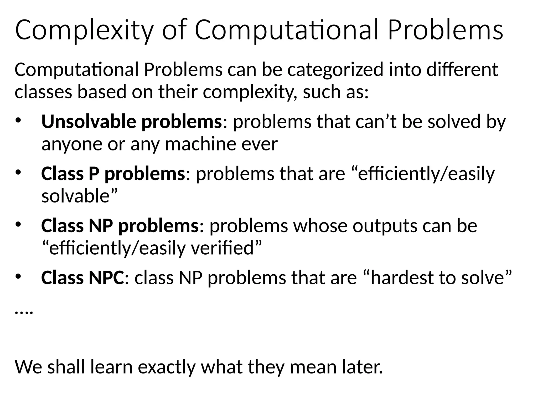
Complexity of ComputationalProblems
Computational Problems can be categorized into different
classes based on their complexity, such as:
• Unsolvable problems: problems that can’t be solved by
anyone or any machine ever
• Class P problems: problems that are “efficiently/easily
solvable”
• Class NP problems: problems whose outputs can be
“efficiently/easily verified”
• Class NPC: class NP problems that are “hardest to solve”
….
We shall learn exactly what they mean later.
12.
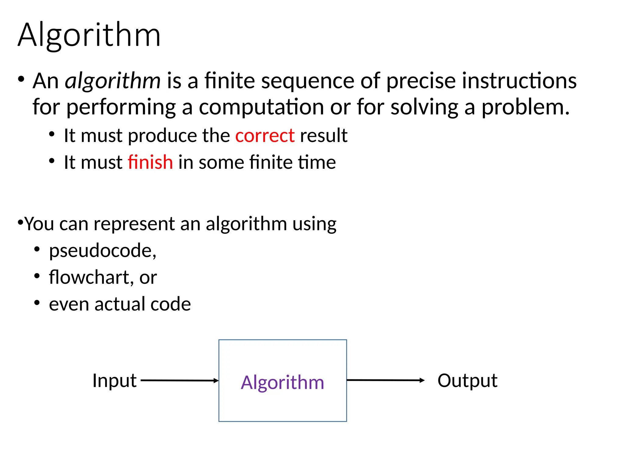
Algorithm
• An algorithmis a finite sequence of precise instructions
for performing a computation or for solving a problem.
• It must produce the correct result
• It must finish in some finite time
•You can represent an algorithm using
• pseudocode,
• flowchart, or
• even actual code
Algorithm
Input Output
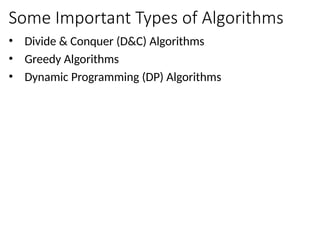
Some Important Typesof Algorithms
• Divide & Conquer (D&C) Algorithms
• Greedy Algorithms
• Dynamic Programming (DP) Algorithms
15.
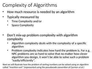
Complexity of Algorithms
•How much resource is needed by an algorithm
• Typically measured by
• Time Complexity and/or
• Space Complexity
• Don’t mix-up problem complexity with algorithm
complexity
• Algorithm complexity deals with the complexity of a specific
algorithm
• Problem complexity indicates how hard the problem is. For e.g.
NPC problems are so hard to solve that no matter how clever
algorithm you design, it won’t be able to solve such a problem
“easily/efficiently”.
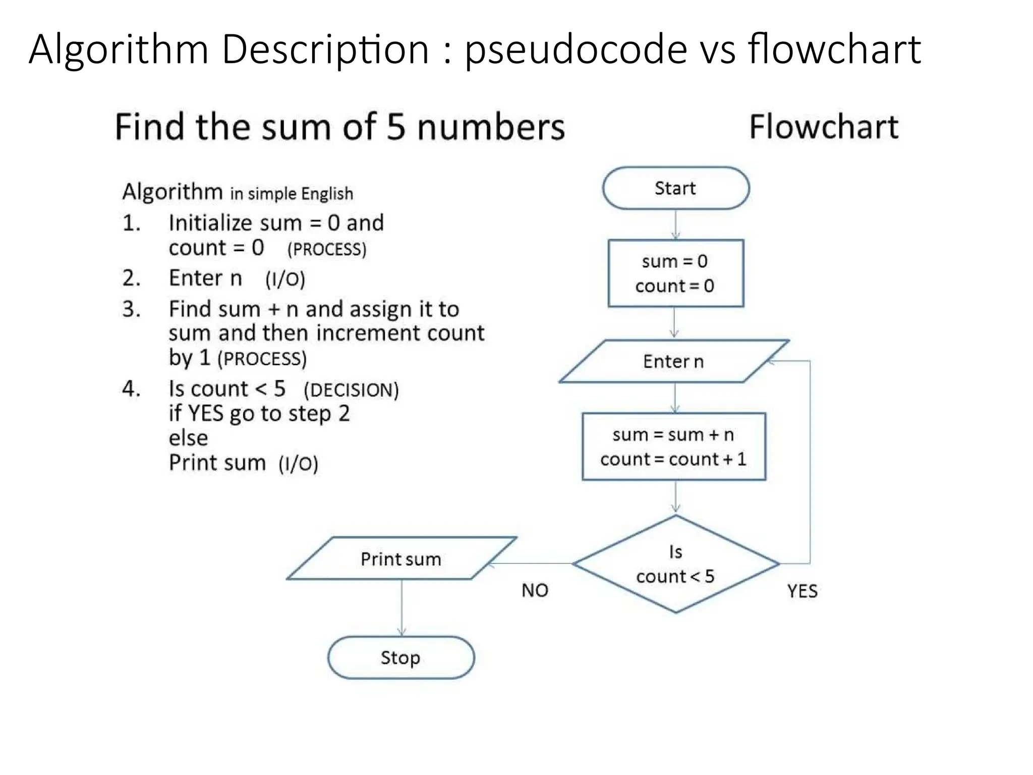
Next we will illustrate how the problem of sorting numbers can be solved using an algorithm
called “insertion-sort” (represented using the pseudocode convention of Cormen et al.)
16.
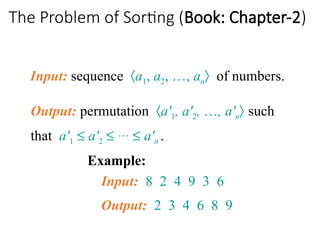
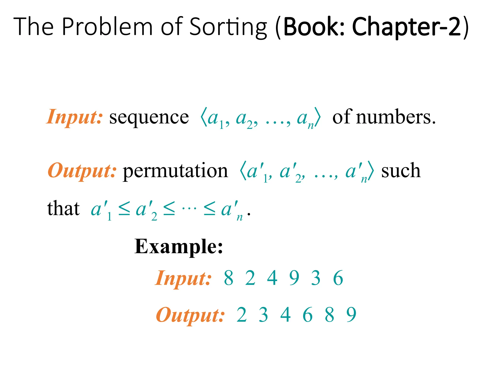
The Problem ofSorting (Book: Chapter-2)
Input: sequence áa1, a2, …, anñ of numbers.
Example:
Input: 8 2 4 9 3 6
Output: 2 3 4 6 8 9
Output: permutation áa'1, a'2, …, a'nñ such
that a'1 £ a'2 £ … £ a'n .
17.
Insertion Sort Pseudocode
INSERTION-SORT(A, n) ⊳ A[1 . . n]
for j ← 2 to n
do ⊳ Insert A[ j ] into the sorted subarray A[1..j -1]
⊳ in such a position that A[1..j] becomes sorted
key ← A[ j]
i ← j – 1
while i > 0 and A[i] > key
do A[i+1] ← A[i]
i ← i – 1
A[i+1] ← key
Comment
Algorithm Name with parameters
(like a C function-header)
Algorithm
body
For
loop
body
While
Loop
body
void insertionSort (int A[], int n)
{ //here A[0 . . n] is an int array
int i, j;
for (j = 2; j<=n; j++) {
key = A[ j];
i = j – 1;
while(i > 0 && A[i] > key){
A[i+1] = A[i];
i = i – 1;
}//while
A[i+1] = key;
}//for
}
Equivalent CPP function
A[0] unused, valid
elements: A[1] … A[n]
Indentation/spacing determines where
the algorithm/loop/if/else-body ends
18.
Insertion Sort Simulation
INSERTION-SORT(A, n) ⊳ A[1 . . n]
for j ← 2 to n
do ⊳ Insert A[ j ] into the sorted subarray A[1..j -1]
⊳ in such a position that A[1..j] becomes sorted
key ← A[ j]
i ← j – 1
while i > 0 and A[i] > key
do A[i+1] ← A[i]
i ← i – 1
A[i+1] ← key
i j
1 2 3 4 5
7 4 9 5 1
4
key
i j
1 2 3 4 5
4 7 9 5 1
9
key
i j
1 2 3 4 5
4 7 9 5 1
5
key
i j
1 2 3 4 5
4 5 7 9 1
1
key
1 2 3 4 5
1 4 5 7 9
Loop Invariant: At the beginning of each iteration
of the for loop, A[1..j-1] is already sorted
See Cormen Book (pp. 18-19) for the proof
Conclusion: when the for loop ends, j=n+1; so according to
the loop invariant, A[1..(n+1-1)]=A[1..n]=A is sorted
19.
Exercise
Q. Write thepseudo-code of the following algorithm
Algorithm Binary-Search(A, n, key):
//returns true if key is found in A[1..n]
20.
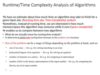
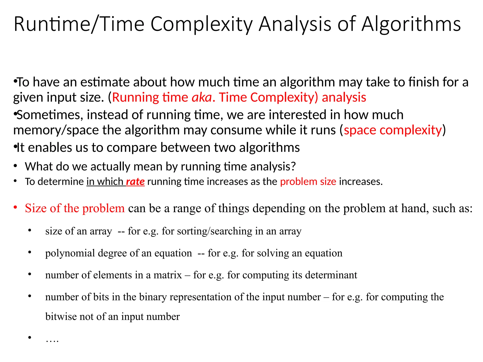
Runtime/Time Complexity Analysisof Algorithms
•To have an estimate about how much time an algorithm may take to finish for a
given input size. (Running time aka. Time Complexity) analysis
•Sometimes, instead of running time, we are interested in how much
memory/space the algorithm may consume while it runs (space complexity)
•It enables us to compare between two algorithms
• What do we actually mean by running time analysis?
• To determine in which rate running time increases as the problem size increases.
• Size of the problem can be a range of things depending on the problem at hand, such as:
• size of an array -- for e.g. for sorting/searching in an array
• polynomial degree of an equation -- for e.g. for solving an equation
• number of elements in a matrix – for e.g. for computing its determinant
• number of bits in the binary representation of the input number – for e.g. for computing the
bitwise not of an input number
• ….
21.
Informal Notion ofRunning Time
• Express runtime as a function of the input size n (i.e., as a function, f(n)) in order
to understand how f(n) grows with n and
• count only the most significant term of f(n) and ignore everything else (because
those won’t affect running time much for very large values of n).
Thus the running times (also called time complexity) of the programs of the previous
slide becomes:
f(N)= c1N ≤ N*(some constant)
g(N) = (c1+c2+c3)N+(c1+c2) ≤ (c1+c2+c3)N = N*(some constant)
Thus both these functions are bounded (from above) by some constant multiple of
N and as such both have the same upper bound: O(N). This means that, the running
time of each of these algorithms is always less than or equal to a constant multiple of
N; we ignore the values of constants in the Big Oh notation, i.e., we never write
O(543N) [it is actually O(N)] or O(65N2
+34N+7) [it is actually O(N2
)].
We compare running times of different algorithms in an asymptotic manner (i.e., we
check if f(n) > g(n) for very large values of n). That’s why, the task of computing
time complexity (of an algorithm) is also called asymptotic analysis.
22.
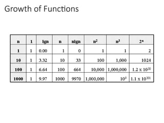
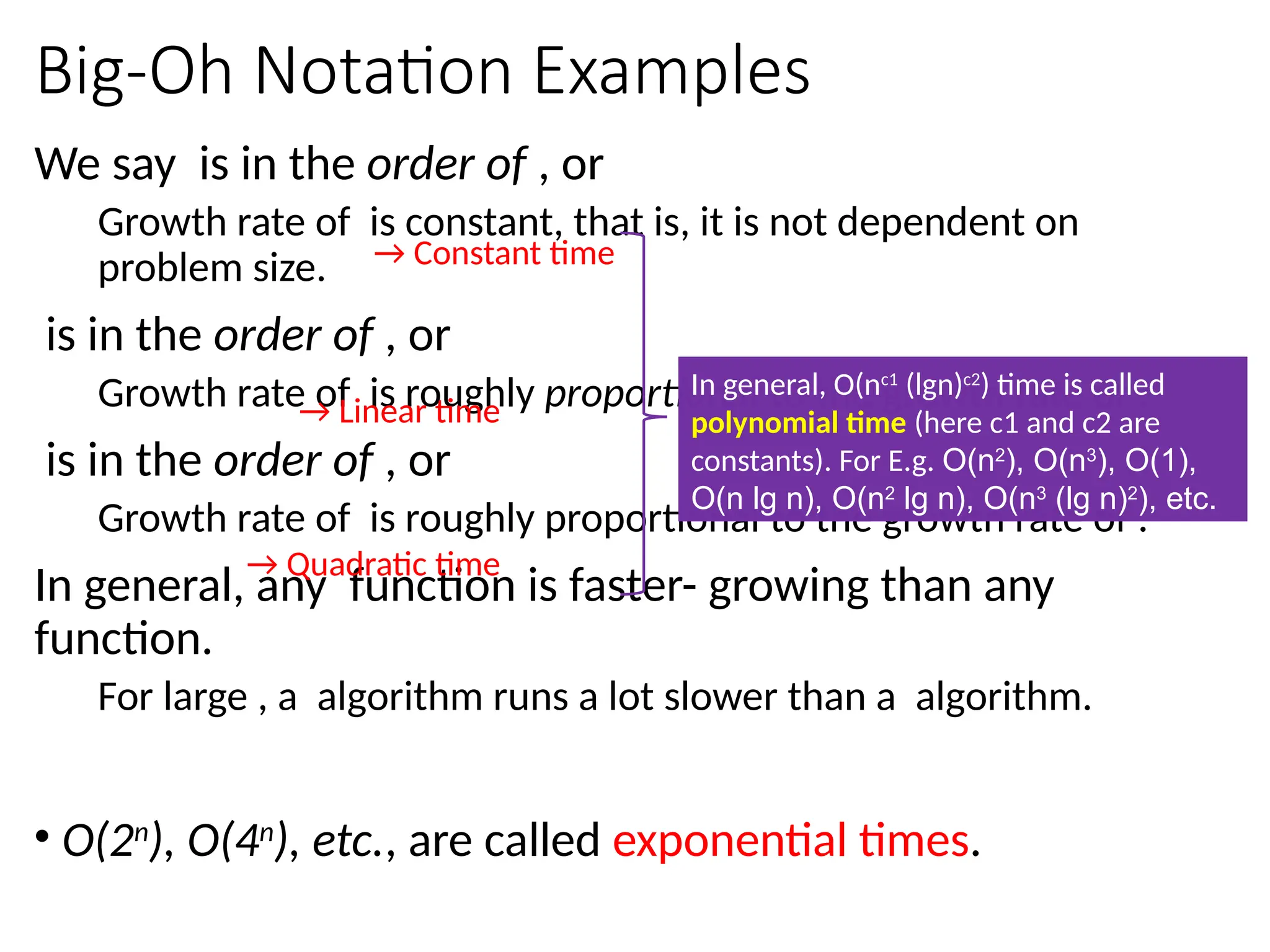
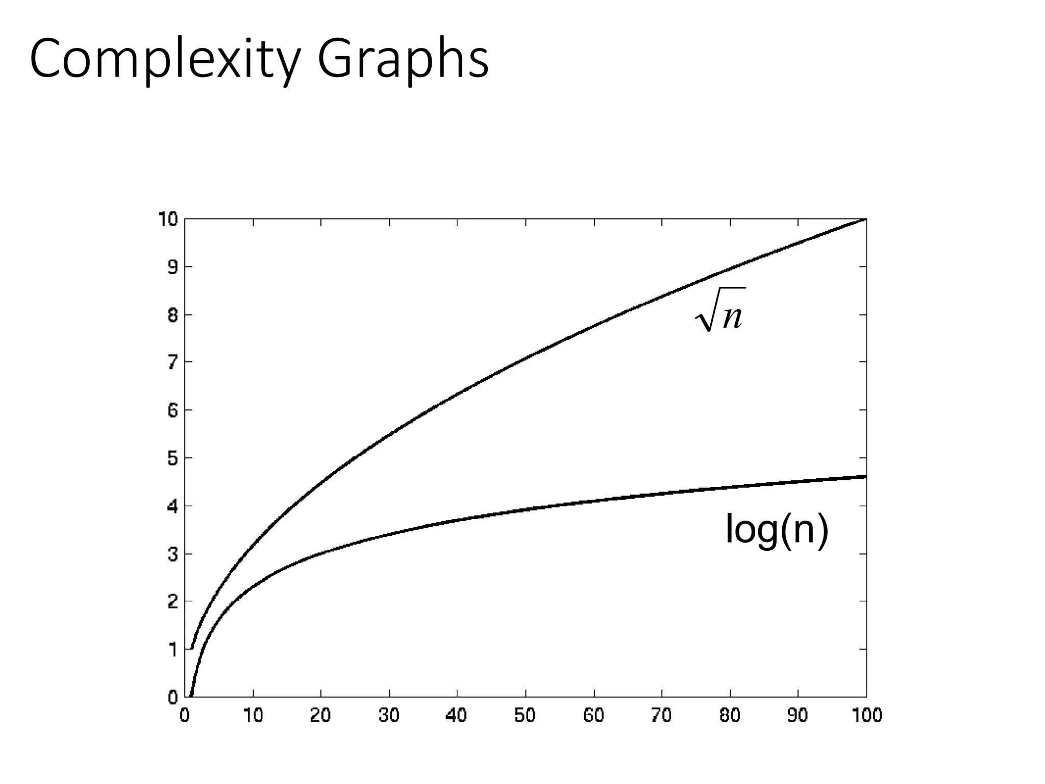
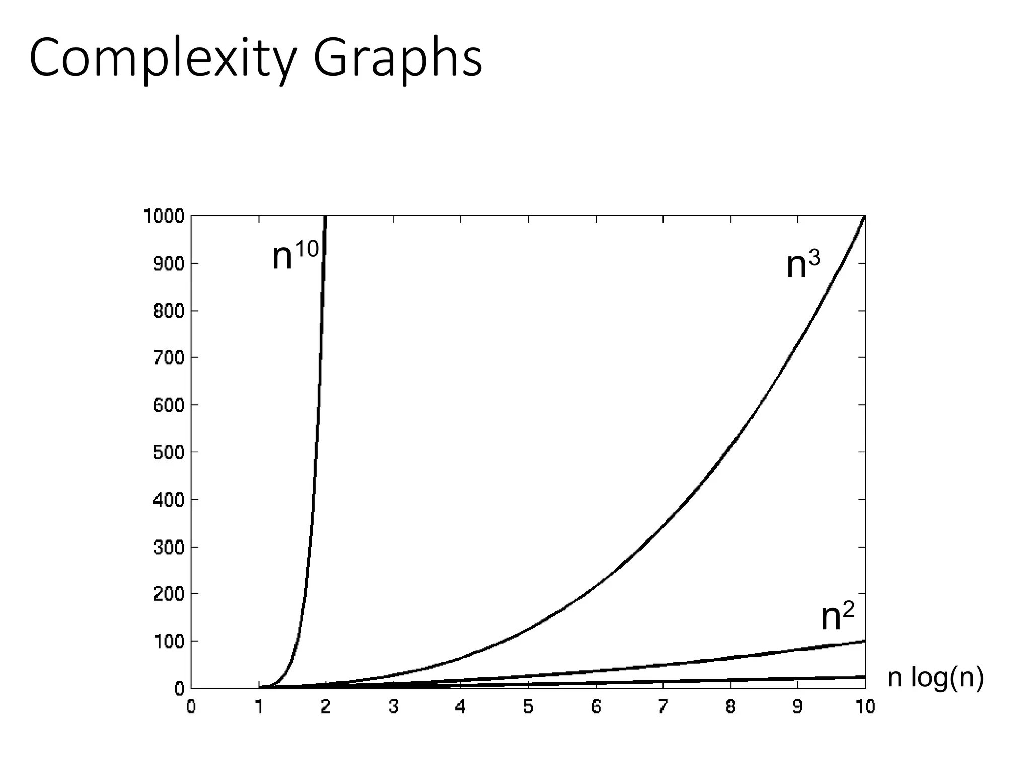
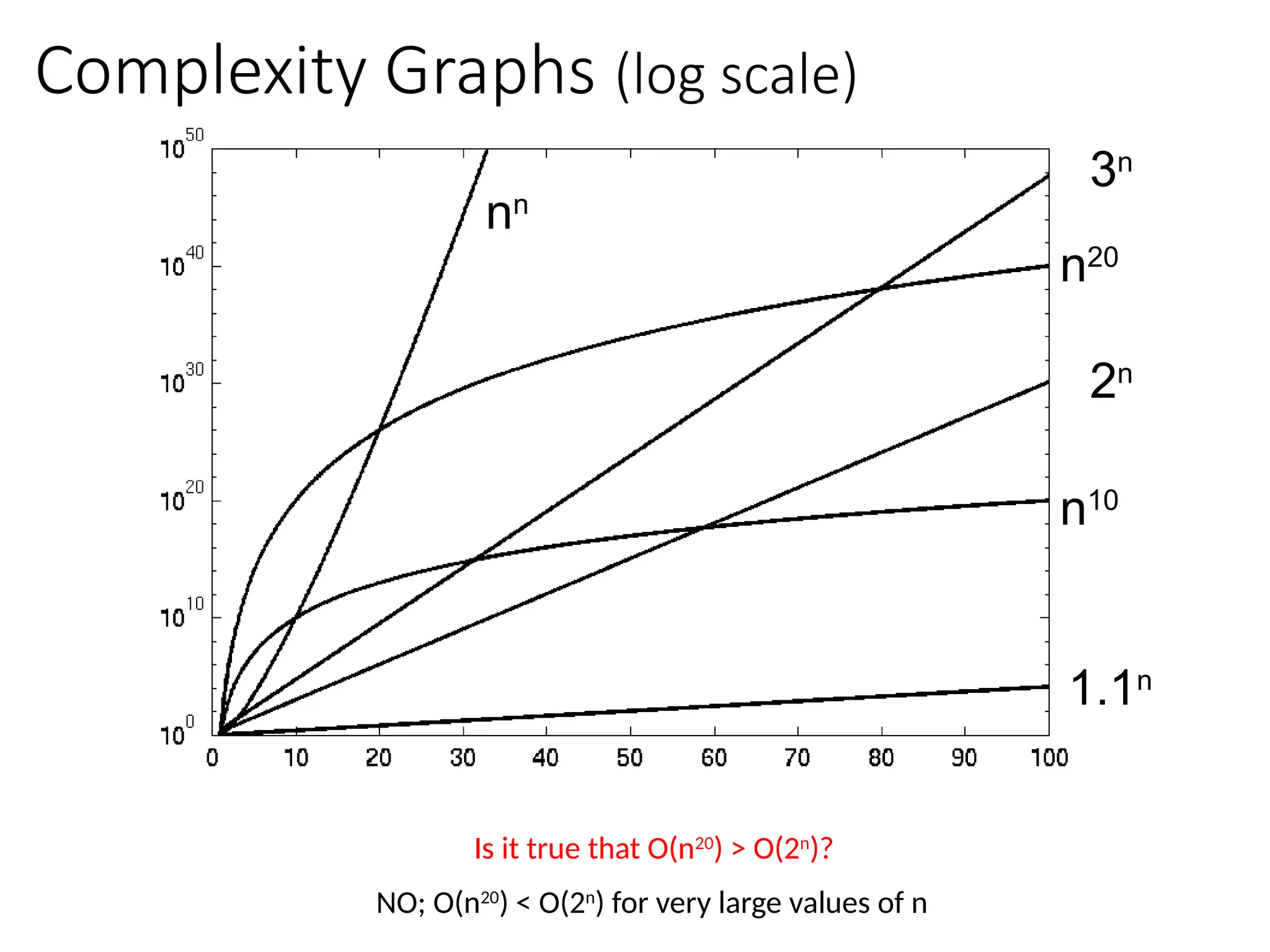
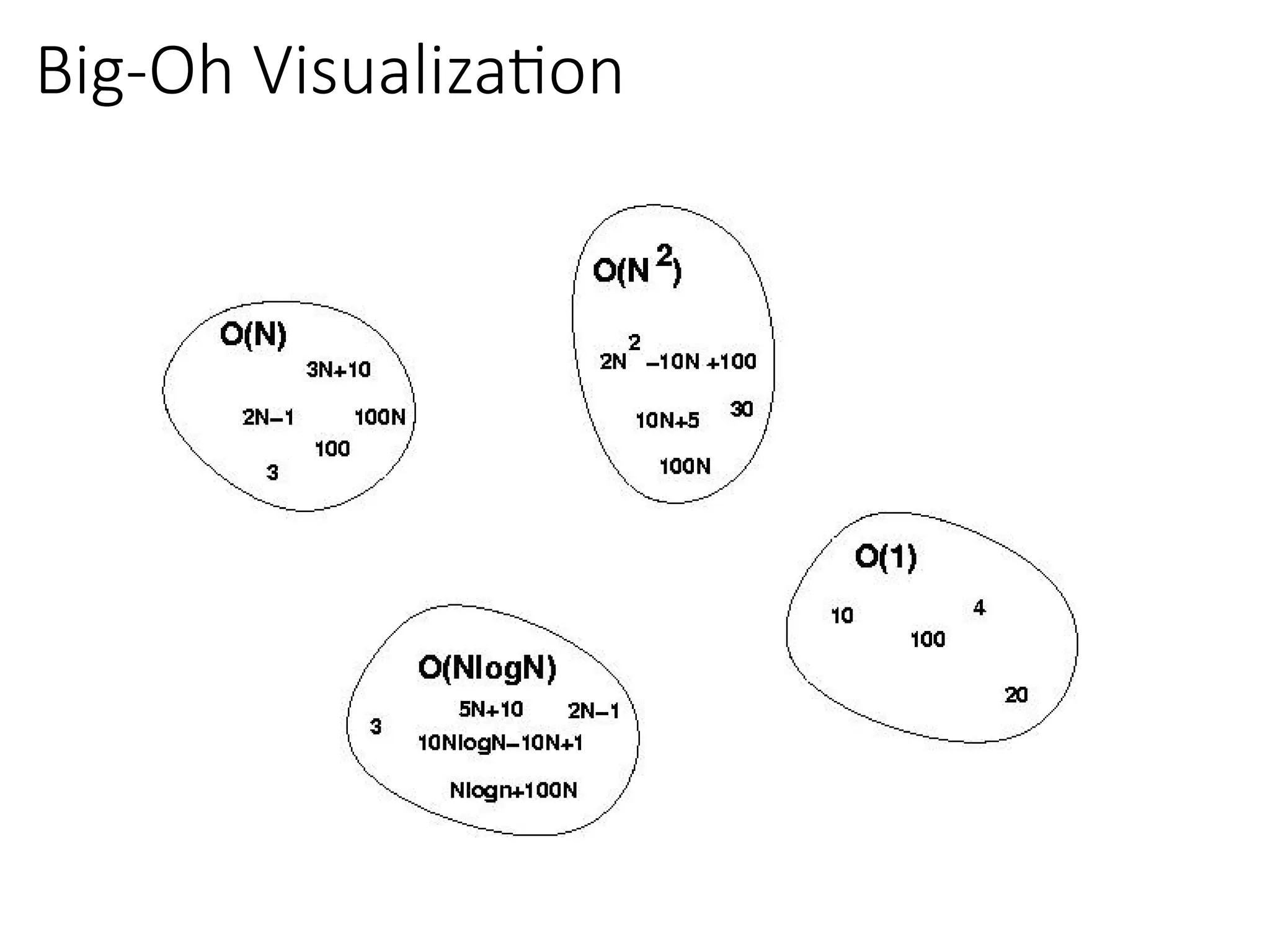
Big-Oh Notation Examples
Wesay is in the order of , or
Growth rate of is constant, that is, it is not dependent on
problem size.
is in the order of , or
Growth rate of is roughly proportional to the growth rate of .
is in the order of , or
Growth rate of is roughly proportional to the growth rate of .
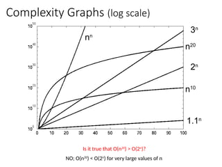
In general, any function is faster- growing than any
function.
For large , a algorithm runs a lot slower than a algorithm.
→ Constant time
→ Linear time
→ Quadratic time
• O(2n
), O(4n
), etc., are called exponential times.
In general, O(nc1
(lgn)c2
) time is called
polynomial time (here c1 and c2 are
constants). For E.g. O(n2
), O(n3
), O(1),
O(n lg n), O(n2
lg n), O(n3
(lg n)2
), etc.
23.
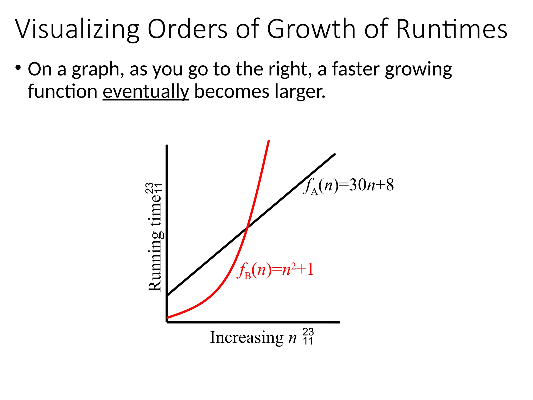
Visualizing Orders ofGrowth of Runtimes
• On a graph, as you go to the right, a faster growing
function eventually becomes larger.
fA(n)=30n+8
Increasing n
fB(n)=n2
+1
Running
time
Asymptotic Notations
O-notation (BigOh)
O(g(n)) is the set of functions
with smaller or same order of
growth as g(n)
Examples:
T(n) = 3n2
+10nlgn+8 is O(n2
), O(n2
lgn), O(n3
), O(n4
), …
T’(n) = 52n2
+3n2
lgn+8 is
Loose upper
bounds
O(n2
lgn), O(n3
), O(n4
), …
This means that f(n) is bounded from above by a constant multiple of g(n)
f(n) is O(g(n))
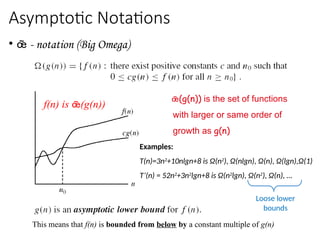
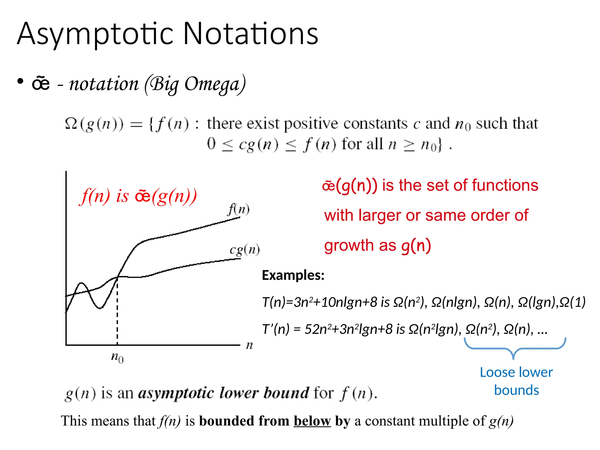
Asymptotic Notations
• - notation (Big Omega)
(g(n)) is the set of functions
with larger or same order of
growth as g(n)
Examples:
T(n)=3n2
+10nlgn+8 is Ω(n2
), Ω(nlgn), Ω(n), Ω(lgn),Ω(1)
T’(n) = 52n2
+3n2
lgn+8 is Ω(n2
lgn), Ω(n2
), Ω(n), …
This means that f(n) is bounded from below by a constant multiple of g(n)
f(n) is (g(n))
Loose lower
bounds
33.
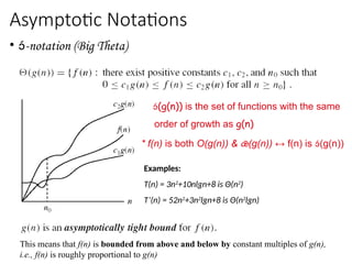
Asymptotic Notations
• -notation(Big Theta)
(g(n)) is the set of functions with the same
order of growth as g(n)
* f(n) is both O(g(n)) & (g(n)) ↔ f(n) is (g(n))
Examples:
T(n) = 3n2
+10nlgn+8 is Θ(n2
)
T’(n) = 52n2
+3n2
lgn+8 is Θ(n2
lgn)
This means that f(n) is bounded from above and below by constant multiples of g(n),
i.e., f(n) is roughly proportional to g(n)
34.
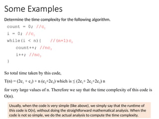
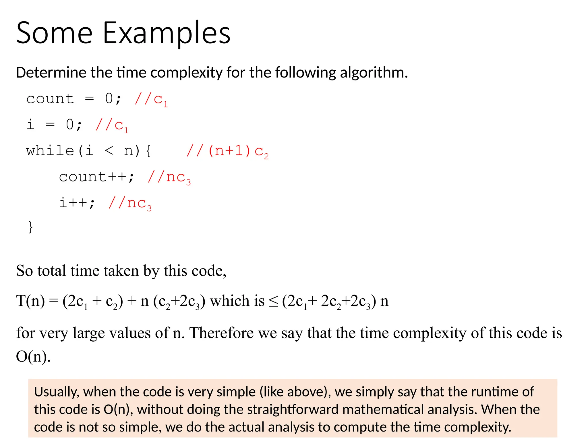
Some Examples
Determine thetime complexity for the following algorithm.
count = 0; //c1
i = 0; //c1
while(i < n){ //(n+1)c2
count++; //nc3
i++; //nc3
}
So total time taken by this code,
T(n) = (2c1 + c2) + n (c2+2c3) which is ≤ (2c1+ 2c2+2c3) n
for very large values of n. Therefore we say that the time complexity of this code is
O(n).
Usually, when the code is very simple (like above), we simply say that the runtime of
this code is O(n), without doing the straightforward mathematical analysis. When the
code is not so simple, we do the actual analysis to compute the time complexity.
35.
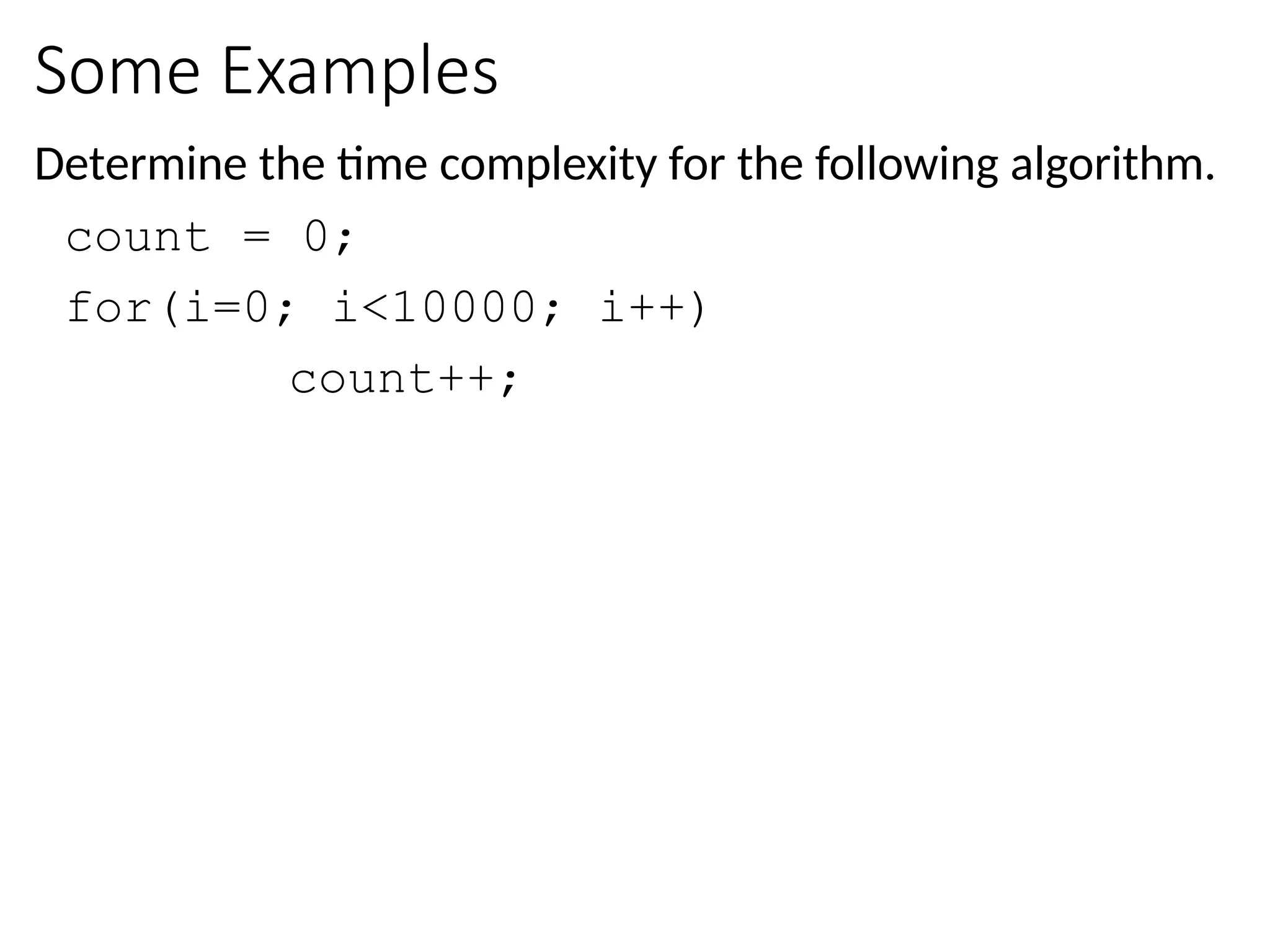
Some Examples
Determine thetime complexity for the following algorithm.
count = 0;
for(i=0; i<10000; i++)
count++;
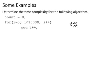
36.
Some Examples
Determine thetime complexity for the following algorithm.
count = 0;
for(i=0; i<10000; i++)
count++;
(1)
37.
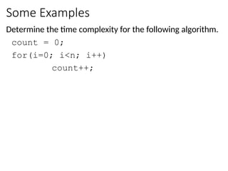
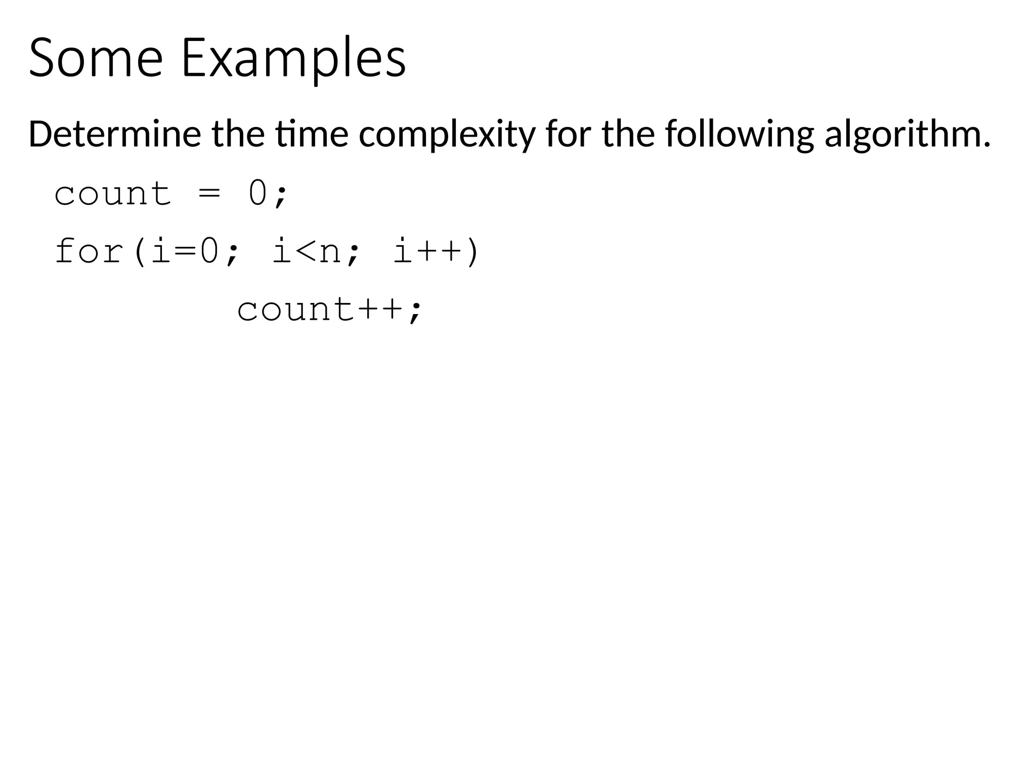
Some Examples
Determine thetime complexity for the following algorithm.
count = 0;
for(i=0; i<n; i++)
count++;
38.
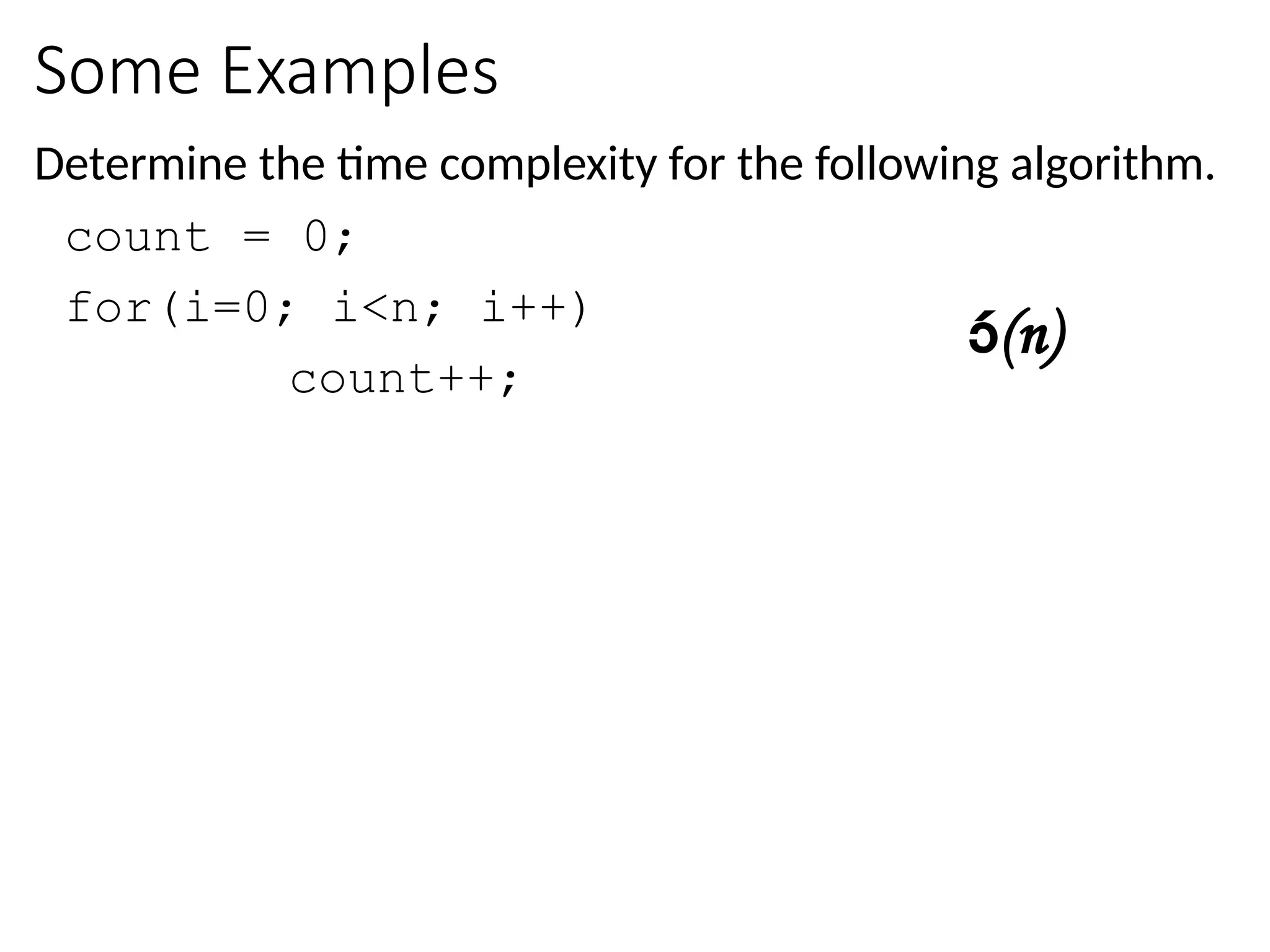
Some Examples
Determine thetime complexity for the following algorithm.
count = 0;
for(i=0; i<n; i++)
count++;
(n)
39.
Some Examples
Determine thetime complexity for the following algorithm.
sum = 0;
for(i=0; i<n; i++)
for(j=0; j<n; j++)
sum += arr[i][j];
40.
Some Examples
Determine thetime complexity for the following algorithm.
sum = 0;
for(i=0; i<n; i++)
for(j=0; j<n; j++)
sum += arr[i][j];
(n2
)
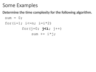
41.
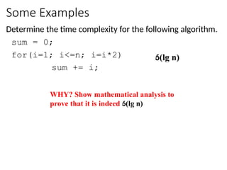
Some Examples
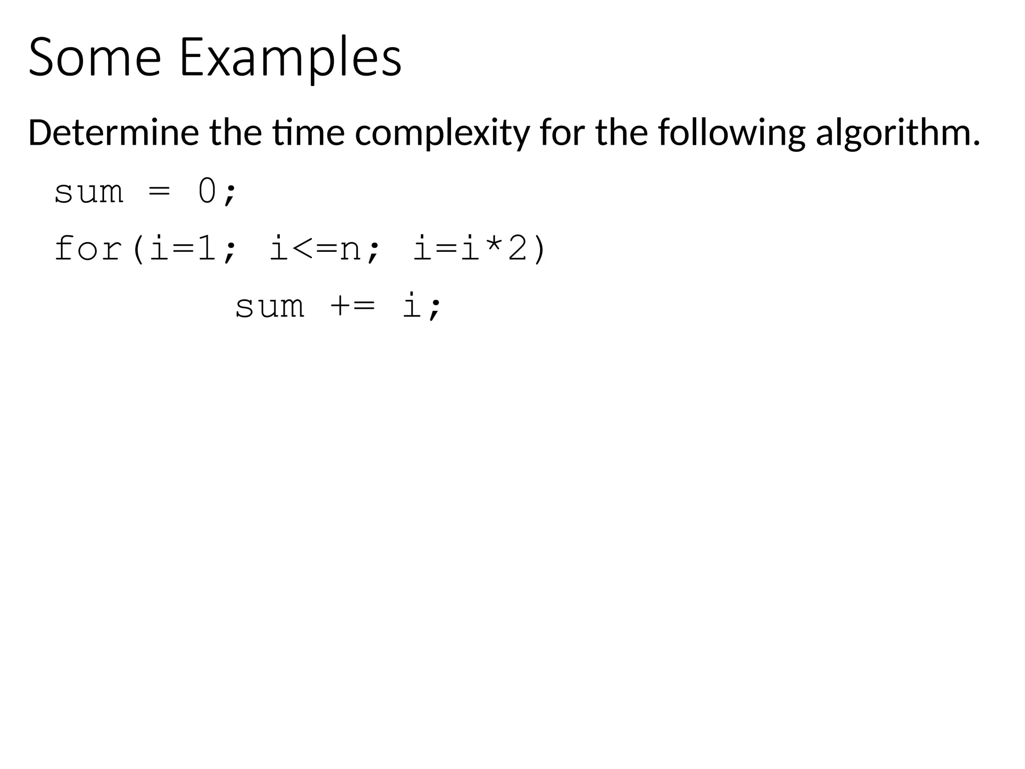
Determine thetime complexity for the following algorithm.
sum = 0;
for(i=1; i<=n; i=i*2)
sum += i;
42.
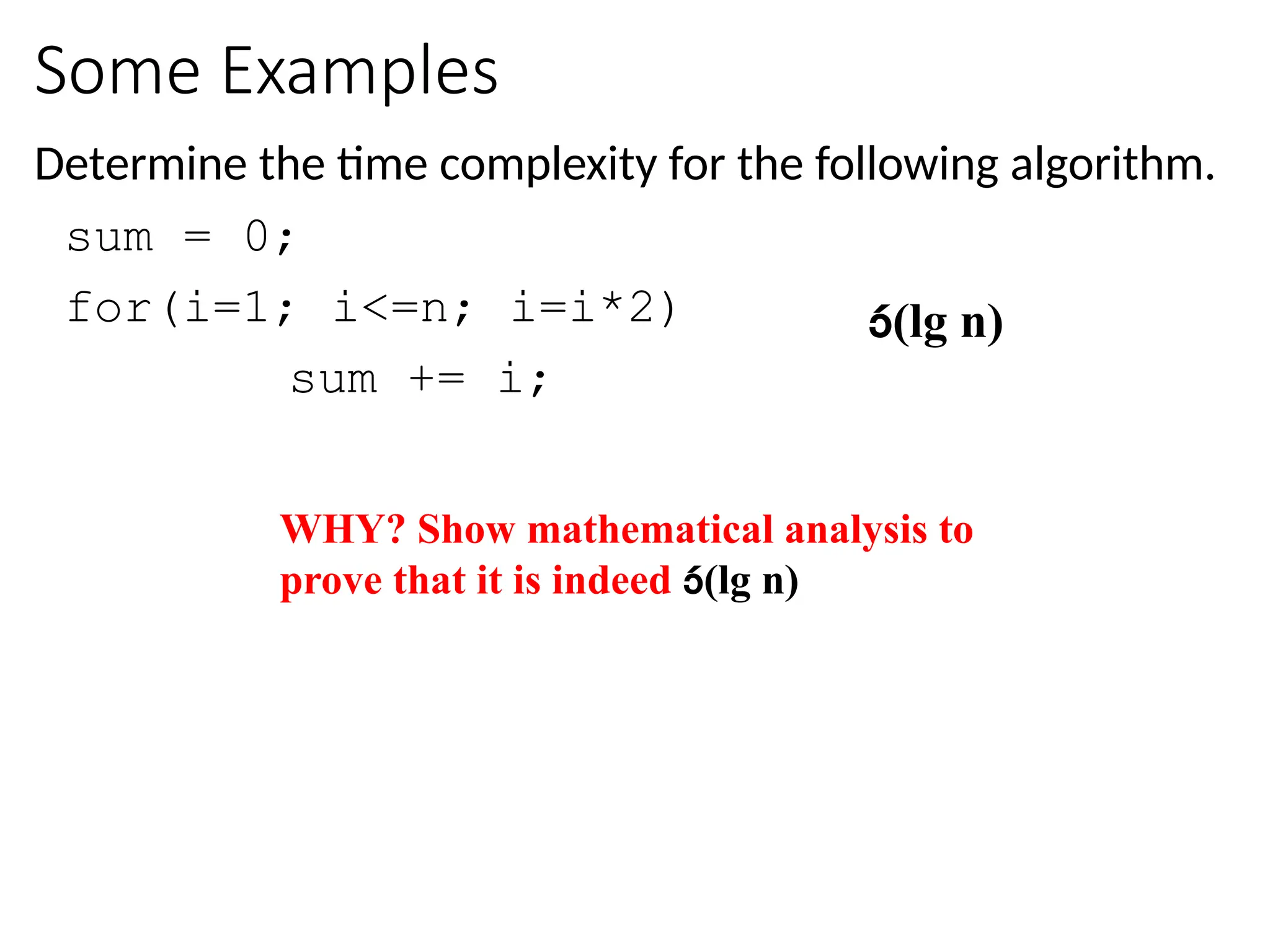
Some Examples
Determine thetime complexity for the following algorithm.
sum = 0;
for(i=1; i<=n; i=i*2)
sum += i;
(lg n)
WHY? Show mathematical analysis to
prove that it is indeed (lg n)
43.
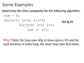
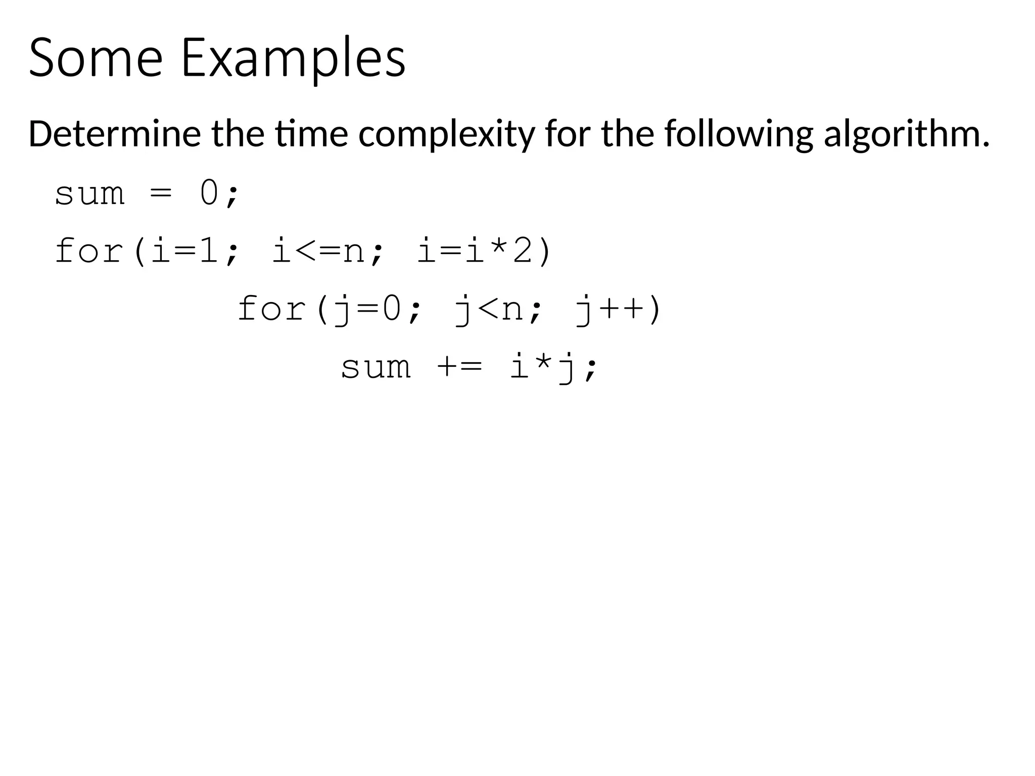
Some Examples
Determine thetime complexity for the following algorithm.
sum = 0;
for(i=1; i<=n; i=i*2)
for(j=0; j<n; j++)
sum += i*j;
44.
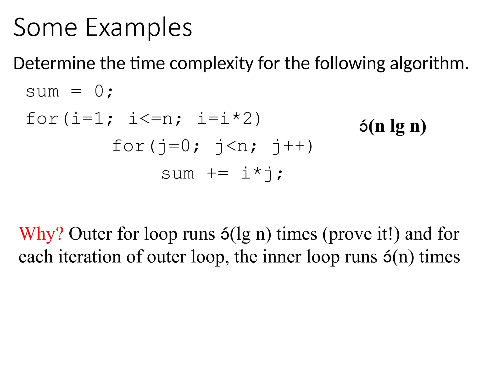
Some Examples
Determine thetime complexity for the following algorithm.
sum = 0;
for(i=1; i<=n; i=i*2)
for(j=0; j<n; j++)
sum += i*j;
(n lg n)
Why? Outer for loop runs (lg n) times (prove it!) and for
each iteration of outer loop, the inner loop runs (n) times
45.
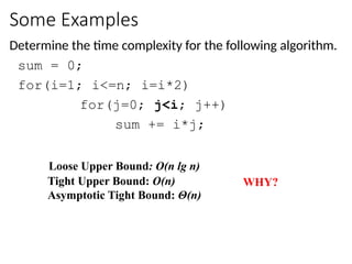
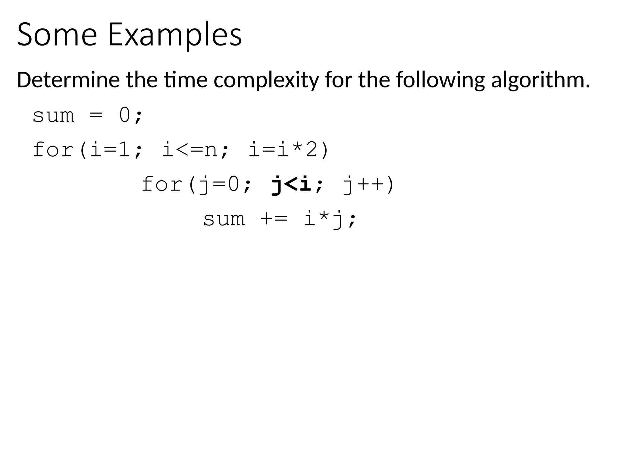
Some Examples
Determine thetime complexity for the following algorithm.
sum = 0;
for(i=1; i<=n; i=i*2)
for(j=0; j<i; j++)
sum += i*j;
46.
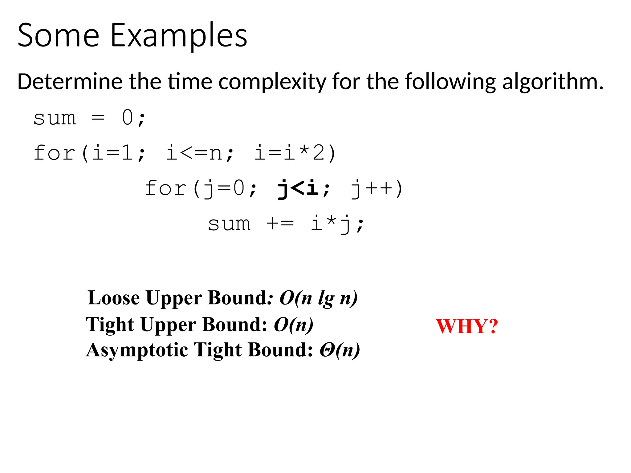
Some Examples
Determine thetime complexity for the following algorithm.
sum = 0;
for(i=1; i<=n; i=i*2)
for(j=0; j<i; j++)
sum += i*j;
Loose Upper Bound: O(n lg n)
WHY?
Tight Upper Bound: O(n)
Asymptotic Tight Bound: Θ(n)
47.
Does implementation matter?
Determinethe time complexity for the following algorithm.
char str[100];
gets(str); //let strlen(str) = n
for(i=0; i<strlen(str); i++)
str[i] -= 32;
48.
Does implementation matter?
Determinethe time complexity for the following algorithm.
char someString[10];
gets(someString);
for(i=0; i<strlen(someString); i++)
someString[i] -= 32;
(n2
)
49.
Does implementation matter?
charsomeString[10];
gets(someString);
for(i=0; i<strlen(someString); i++)
someString[i] -= 32;
Can we re-implement it to make it more efficient?
char someString[10];
gets(someString);
int t = strlen(someString);
for(i=0; i<t; i++)
someString[i] -= 32;
(n2
)
This example shows that a badly implemented algorithm may have
greater time complexity than a more efficient implementation
(n)
YES
50.
int find_a(char *str)
{
inti;
for (i = 0; str[i]; i++)
{
if (str[i] == ’a’)
return i;
}
return -1;
}
Time complexity:
Consider two inputs: “alibi” and “never”
What is the time complexity of the above algorithm?
Depends on the input (str):
• (1) for best possible input which starts with ‘a’ e.g. when str = “alibaba”
• (n) for worst possible input which doesn’t contain any ‘a’ e.g. when str = “nitin”
So far, we have been able to ALWAYS determine time complexity of an
algorithm from the input size only. But is input size enough to
determine time complexity unambiguously?
51.
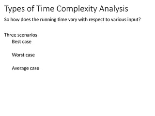
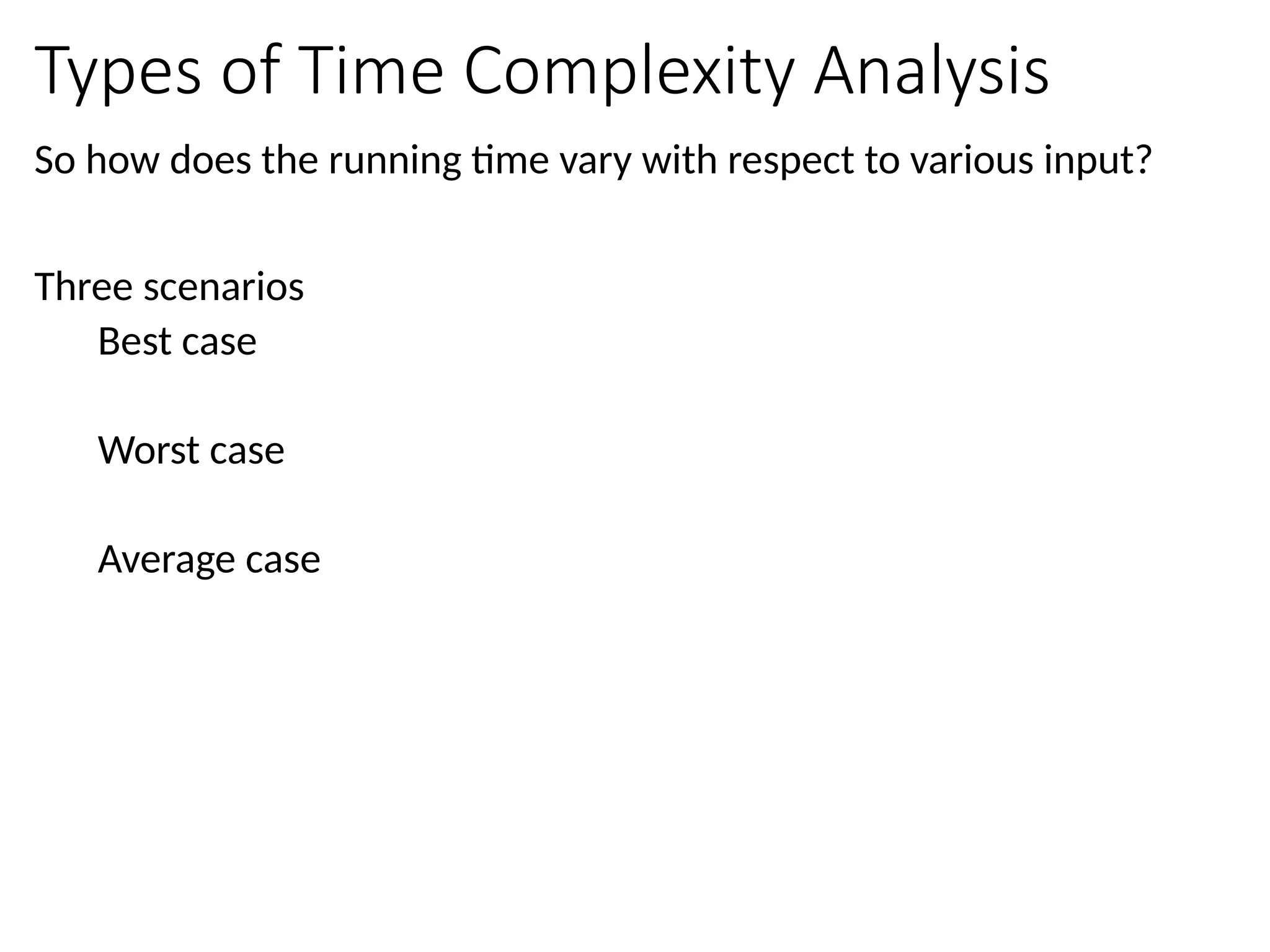
Types of TimeComplexity Analysis
So how does the running time vary with respect to various input?
Three scenarios
Best case
Worst case
Average case
52.
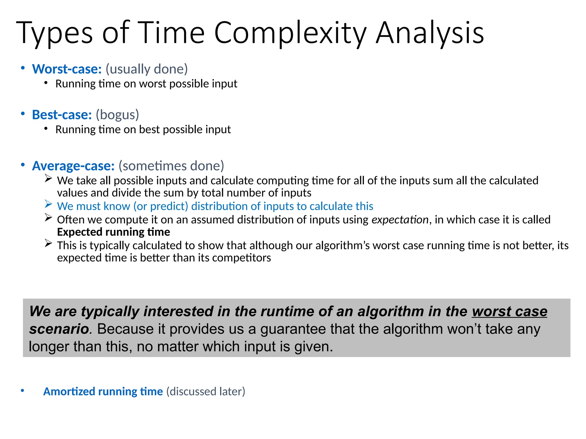
Types of TimeComplexity Analysis
• Worst-case: (usually done)
• Running time on worst possible input
• Best-case: (bogus)
• Running time on best possible input
• Average-case: (sometimes done)
We take all possible inputs and calculate computing time for all of the inputs sum all the calculated
values and divide the sum by total number of inputs
We must know (or predict) distribution of inputs to calculate this
Often we compute it on an assumed distribution of inputs using expectation, in which case it is called
Expected running time
This is typically calculated to show that although our algorithm’s worst case running time is not better, its
expected time is better than its competitors
• Amortized running time (discussed later)
We are typically interested in the runtime of an algorithm in the worst case
scenario. Because it provides us a guarantee that the algorithm won’t take any
longer than this, no matter which input is given.
53.
Is input sizeeverything that matters?
int find_a(char *str)
{
int i;
for (i = 0; str[i]; i++)
{
if (str[i] == ’a’)
return i;
}
return -1;
}
Time complexity:
Consider two inputs: “alibi” and “never”
Example of Best & Worst Case Analysis
Best case input: strings that contain an ‘a’ in its first index
Best case time complexity: O(1)
Worst case input: strings that do not contain any ‘a’
Worst case time complexity: O(n)
Average time complexity: O(n), how?
54.
Insertion Sort AlgorithmRevisited
INSERTION-SORT (A, n) ⊳ A[1 . . n]
for j ← 2 to n
do key ← A[ j]
i ← j – 1
while i > 0 and A[i]
> key
do A[i+1]
← A[i]
i ← i –
1
A[i+1] = key
What is the time complexity?
Depends on arrangement of numbers in the input array.
How can you arrange the input numbers so that this algorithm
becomes most inefficient (worst case)?
How can you arrange the input numbers so that this algorithm
becomes most efficient (best case)?
55.
Insertion Sort: RunningTime
Statement
cost
INSERTION-SORT (A, n) ⊳ A[1 . . n]
for j ← 2 to n
do key ← A[ j]
i ← j – 1
while i > 0 and A[i] > key
do A[i+1] ← A[i]
i ← i – 1
A[i+1] = key
𝑇(𝑛)=𝑐1𝑛+𝑐2(𝑛−1)+𝑐3(𝑛−1)+𝑐4∑
𝑗=2
𝑛
𝑡𝑗+𝑐5 ∑
𝑗=2
𝑛
(𝑡𝑗−1)+𝑐6∑
𝑗=2
𝑛
(𝑡𝑗−1)+𝑐7 (𝑛−1)
Here tj = no. of times the condition of while loop is tested for the current value of j.
How can we simplify T(n)? Hint: compute the value of T(n) in the best/worst case
56.
Insertion Sort: RunningTime
Statement
cost
INSERTION-SORT (A, n) ⊳ A[1 . . n]
for j ← 2 to n
do key ← A[ j]
i ← j – 1
while i > 0 and A[i] > key
do A[i+1] ← A[i]
i ← i – 1
A[i+1] = key
𝑇(𝑛)=𝑐1𝑛+𝑐2(𝑛−1)+𝑐3(𝑛−1)+𝑐4∑
𝑗=2
𝑛
𝑡𝑗+𝑐5 ∑
𝑗=2
𝑛
(𝑡𝑗−1)+𝑐6∑
𝑗=2
𝑛
(𝑡𝑗−1)+𝑐7 (𝑛−1)
Here tj = no. of times the condition of while loop is tested for the current value of j.
In the worst case (when input is reverse-sorted), in each iteration of the for loop, all the j-1
elements need to be right shifted, i.e., tj=(j-1)+1 = j :[1 is added to represent the last test].
Putting this in the above eq., we get: T(n) = An2
+Bn+C → O(n2
), where A, B, C are constants.
What is T(n) in the best case (when the input numbers are already sorted)?
If you are asked to compute worst case time of Insertion-Sort, just say that the while loop
runs j times for worst possible input i.e. reverse sorted array (explain why) and then
compute T(n) from T(n) = Σn
j=2 (j) = …. = n(n+1)/2 – 1 which is O(n2
)
You don’t really need to show such a detailed calculation as shown here & in the book.
57.
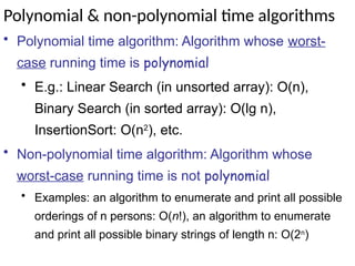
Polynomial & non-polynomialtime algorithms
• Polynomial time algorithm: Algorithm whose worst-
case running time is polynomial
• E.g.: Linear Search (in unsorted array): O(n),
Binary Search (in sorted array): O(lg n),
InsertionSort: O(n2
), etc.
• Non-polynomial time algorithm: Algorithm whose
worst-case running time is not polynomial
• Examples: an algorithm to enumerate and print all possible
orderings of n persons: O(n!), an algorithm to enumerate
and print all possible binary strings of length n: O(2n
)
58.
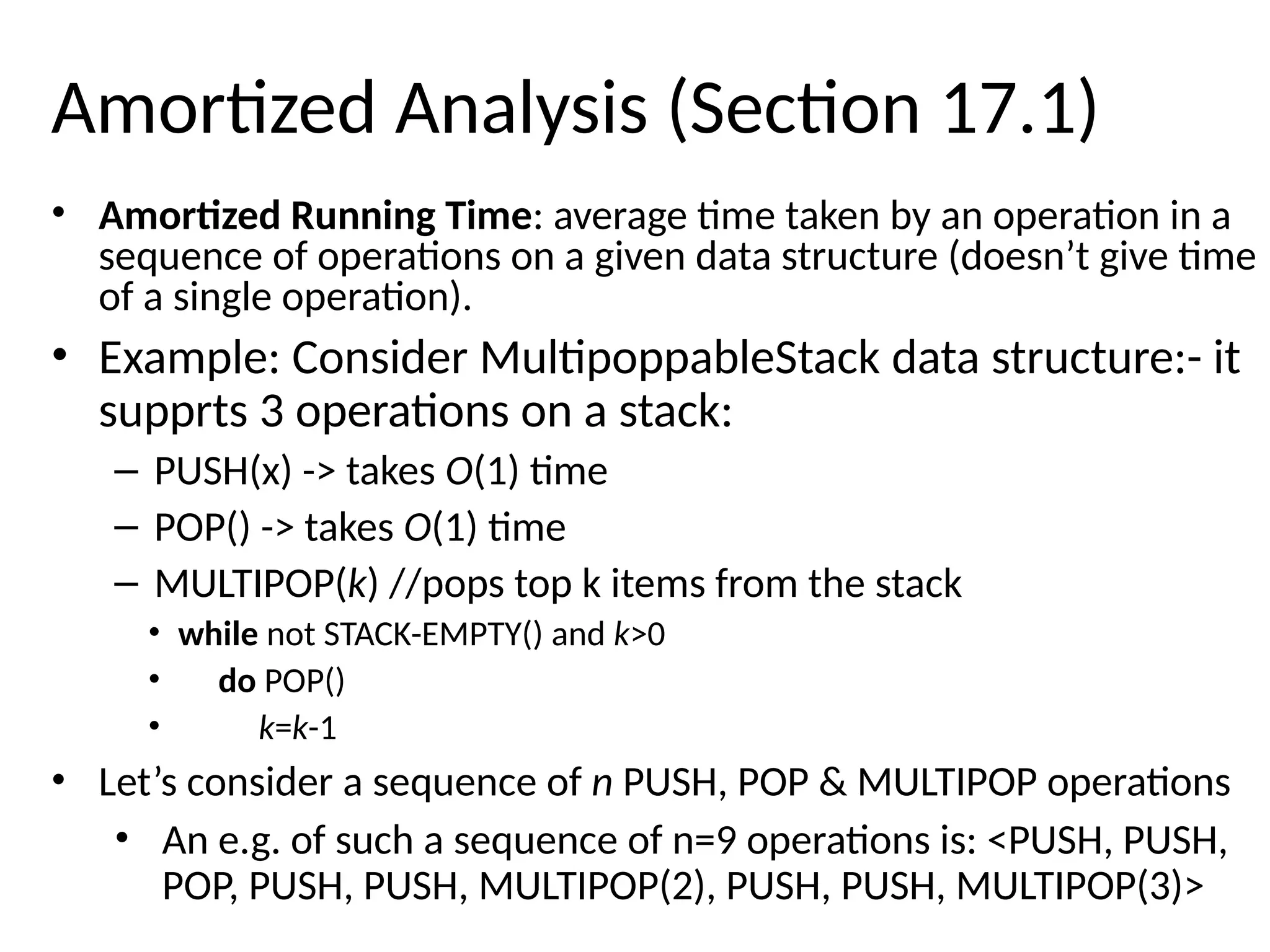
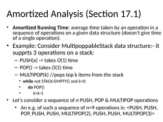
Amortized Analysis (Section17.1)
• Amortized Running Time: average time taken by an operation in a
sequence of operations on a given data structure (doesn’t give time
of a single operation).
• Example: Consider MultipoppableStack data structure:- it
supprts 3 operations on a stack:
– PUSH(x) -> takes O(1) time
– POP() -> takes O(1) time
– MULTIPOP(k) //pops top k items from the stack
• while not STACK-EMPTY() and k>0
• do POP()
• k=k-1
• Let’s consider a sequence of n PUSH, POP & MULTIPOP operations
• An e.g. of such a sequence of n=9 operations is: <PUSH, PUSH,
POP, PUSH, PUSH, MULTIPOP(2), PUSH, PUSH, MULTIPOP(3)>
59.
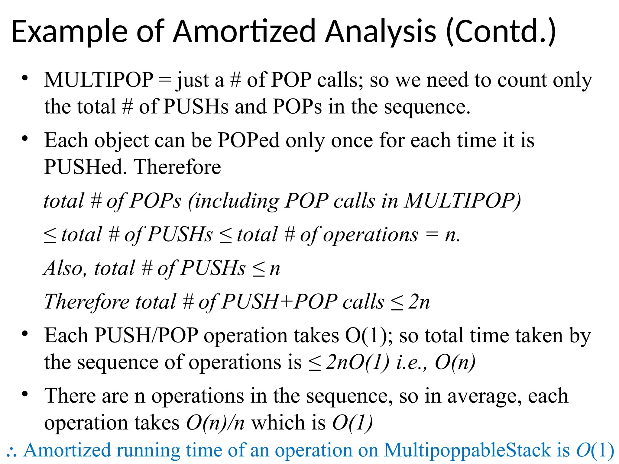
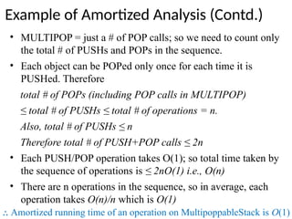
• MULTIPOP =just a # of POP calls; so we need to count only
the total # of PUSHs and POPs in the sequence.
• Each object can be POPed only once for each time it is
PUSHed. Therefore
total # of POPs (including POP calls in MULTIPOP)
≤ total # of PUSHs ≤ total # of operations = n.
Also, total # of PUSHs ≤ n
Therefore total # of PUSH+POP calls ≤ 2n
• Each PUSH/POP operation takes O(1); so total time taken by
the sequence of operations is ≤ 2nO(1) i.e., O(n)
• There are n operations in the sequence, so in average, each
operation takes O(n)/n which is O(1)
⸫ Amortized running time of an operation on MultipoppableStack is O(1)
Example of Amortized Analysis (Contd.)
![Computational Problem
A computational problem can be represented as a question
that describes the requirements of the desired output given
an input. For e.g.
• Is n a prime number? (n is a user input)
• What are the prime factors of n? (n is a user input)
• How many prime factors of n are there? (n is user input)
• What is the maximum value of a[i]? (a[1…n] is an input
array)](https://image.slidesharecdn.com/l1algobasics-250408141822-6fb704f9/85/L1_Start_of_Learning_of_Algorithms_Basics-pptx-6-320.jpg)


![Insertion Sort Pseudocode
INSERTION-SORT (A, n) ⊳ A[1 . . n]
for j ← 2 to n
do ⊳ Insert A[ j ] into the sorted subarray A[1..j -1]
⊳ in such a position that A[1..j] becomes sorted
key ← A[ j]
i ← j – 1
while i > 0 and A[i] > key
do A[i+1] ← A[i]
i ← i – 1
A[i+1] ← key
Comment
Algorithm Name with parameters
(like a C function-header)
Algorithm
body
For
loop
body
While
Loop
body
void insertionSort (int A[], int n)
{ //here A[0 . . n] is an int array
int i, j;
for (j = 2; j<=n; j++) {
key = A[ j];
i = j – 1;
while(i > 0 && A[i] > key){
A[i+1] = A[i];
i = i – 1;
}//while
A[i+1] = key;
}//for
}
Equivalent CPP function
A[0] unused, valid
elements: A[1] … A[n]
Indentation/spacing determines where
the algorithm/loop/if/else-body ends](https://image.slidesharecdn.com/l1algobasics-250408141822-6fb704f9/85/L1_Start_of_Learning_of_Algorithms_Basics-pptx-17-320.jpg)
![Insertion Sort Simulation
INSERTION-SORT (A, n) ⊳ A[1 . . n]
for j ← 2 to n
do ⊳ Insert A[ j ] into the sorted subarray A[1..j -1]
⊳ in such a position that A[1..j] becomes sorted
key ← A[ j]
i ← j – 1
while i > 0 and A[i] > key
do A[i+1] ← A[i]
i ← i – 1
A[i+1] ← key
i j
1 2 3 4 5
7 4 9 5 1
4
key
i j
1 2 3 4 5
4 7 9 5 1
9
key
i j
1 2 3 4 5
4 7 9 5 1
5
key
i j
1 2 3 4 5
4 5 7 9 1
1
key
1 2 3 4 5
1 4 5 7 9
Loop Invariant: At the beginning of each iteration
of the for loop, A[1..j-1] is already sorted
See Cormen Book (pp. 18-19) for the proof
Conclusion: when the for loop ends, j=n+1; so according to
the loop invariant, A[1..(n+1-1)]=A[1..n]=A is sorted](https://image.slidesharecdn.com/l1algobasics-250408141822-6fb704f9/85/L1_Start_of_Learning_of_Algorithms_Basics-pptx-18-320.jpg)
![Exercise
Q. Write the pseudo-code of the following algorithm
Algorithm Binary-Search(A, n, key):
//returns true if key is found in A[1..n]](https://image.slidesharecdn.com/l1algobasics-250408141822-6fb704f9/85/L1_Start_of_Learning_of_Algorithms_Basics-pptx-19-320.jpg)
![Informal Notion of Running Time
• Express runtime as a function of the input size n (i.e., as a function, f(n)) in order
to understand how f(n) grows with n and
• count only the most significant term of f(n) and ignore everything else (because
those won’t affect running time much for very large values of n).
Thus the running times (also called time complexity) of the programs of the previous
slide becomes:
f(N)= c1N ≤ N*(some constant)
g(N) = (c1+c2+c3)N+(c1+c2) ≤ (c1+c2+c3)N = N*(some constant)
Thus both these functions are bounded (from above) by some constant multiple of
N and as such both have the same upper bound: O(N). This means that, the running
time of each of these algorithms is always less than or equal to a constant multiple of
N; we ignore the values of constants in the Big Oh notation, i.e., we never write
O(543N) [it is actually O(N)] or O(65N2
+34N+7) [it is actually O(N2
)].
We compare running times of different algorithms in an asymptotic manner (i.e., we
check if f(n) > g(n) for very large values of n). That’s why, the task of computing
time complexity (of an algorithm) is also called asymptotic analysis.](https://image.slidesharecdn.com/l1algobasics-250408141822-6fb704f9/85/L1_Start_of_Learning_of_Algorithms_Basics-pptx-21-320.jpg)


![Some Examples
Determine the time complexity for the following algorithm.
sum = 0;
for(i=0; i<n; i++)
for(j=0; j<n; j++)
sum += arr[i][j];](https://image.slidesharecdn.com/l1algobasics-250408141822-6fb704f9/85/L1_Start_of_Learning_of_Algorithms_Basics-pptx-39-320.jpg)
![Some Examples
Determine the time complexity for the following algorithm.
sum = 0;
for(i=0; i<n; i++)
for(j=0; j<n; j++)
sum += arr[i][j];
(n2
)](https://image.slidesharecdn.com/l1algobasics-250408141822-6fb704f9/85/L1_Start_of_Learning_of_Algorithms_Basics-pptx-40-320.jpg)


![Does implementation matter?
Determine the time complexity for the following algorithm.
char str[100];
gets(str); //let strlen(str) = n
for(i=0; i<strlen(str); i++)
str[i] -= 32;](https://image.slidesharecdn.com/l1algobasics-250408141822-6fb704f9/85/L1_Start_of_Learning_of_Algorithms_Basics-pptx-47-320.jpg)
![Does implementation matter?
Determine the time complexity for the following algorithm.
char someString[10];
gets(someString);
for(i=0; i<strlen(someString); i++)
someString[i] -= 32;
(n2
)](https://image.slidesharecdn.com/l1algobasics-250408141822-6fb704f9/85/L1_Start_of_Learning_of_Algorithms_Basics-pptx-48-320.jpg)
![Does implementation matter?
char someString[10];
gets(someString);
for(i=0; i<strlen(someString); i++)
someString[i] -= 32;
Can we re-implement it to make it more efficient?
char someString[10];
gets(someString);
int t = strlen(someString);
for(i=0; i<t; i++)
someString[i] -= 32;
(n2
)
This example shows that a badly implemented algorithm may have
greater time complexity than a more efficient implementation
(n)
YES](https://image.slidesharecdn.com/l1algobasics-250408141822-6fb704f9/85/L1_Start_of_Learning_of_Algorithms_Basics-pptx-49-320.jpg)
![int find_a(char *str)
{
int i;
for (i = 0; str[i]; i++)
{
if (str[i] == ’a’)
return i;
}
return -1;
}
Time complexity:
Consider two inputs: “alibi” and “never”
What is the time complexity of the above algorithm?
Depends on the input (str):
• (1) for best possible input which starts with ‘a’ e.g. when str = “alibaba”
• (n) for worst possible input which doesn’t contain any ‘a’ e.g. when str = “nitin”
So far, we have been able to ALWAYS determine time complexity of an
algorithm from the input size only. But is input size enough to
determine time complexity unambiguously?](https://image.slidesharecdn.com/l1algobasics-250408141822-6fb704f9/85/L1_Start_of_Learning_of_Algorithms_Basics-pptx-50-320.jpg)

![Is input size everything that matters?
int find_a(char *str)
{
int i;
for (i = 0; str[i]; i++)
{
if (str[i] == ’a’)
return i;
}
return -1;
}
Time complexity:
Consider two inputs: “alibi” and “never”
Example of Best & Worst Case Analysis
Best case input: strings that contain an ‘a’ in its first index
Best case time complexity: O(1)
Worst case input: strings that do not contain any ‘a’
Worst case time complexity: O(n)
Average time complexity: O(n), how?](https://image.slidesharecdn.com/l1algobasics-250408141822-6fb704f9/85/L1_Start_of_Learning_of_Algorithms_Basics-pptx-53-320.jpg)
![Insertion Sort Algorithm Revisited
INSERTION-SORT (A, n) ⊳ A[1 . . n]
for j ← 2 to n
do key ← A[ j]
i ← j – 1
while i > 0 and A[i]
> key
do A[i+1]
← A[i]
i ← i –
1
A[i+1] = key
What is the time complexity?
Depends on arrangement of numbers in the input array.
How can you arrange the input numbers so that this algorithm
becomes most inefficient (worst case)?
How can you arrange the input numbers so that this algorithm
becomes most efficient (best case)?](https://image.slidesharecdn.com/l1algobasics-250408141822-6fb704f9/85/L1_Start_of_Learning_of_Algorithms_Basics-pptx-54-320.jpg)
![Insertion Sort: Running Time
Statement
cost
INSERTION-SORT (A, n) ⊳ A[1 . . n]
for j ← 2 to n
do key ← A[ j]
i ← j – 1
while i > 0 and A[i] > key
do A[i+1] ← A[i]
i ← i – 1
A[i+1] = key
𝑇(𝑛)=𝑐1𝑛+𝑐2(𝑛−1)+𝑐3(𝑛−1)+𝑐4∑
𝑗=2
𝑛
𝑡𝑗+𝑐5 ∑
𝑗=2
𝑛
(𝑡𝑗−1)+𝑐6∑
𝑗=2
𝑛
(𝑡𝑗−1)+𝑐7 (𝑛−1)
Here tj = no. of times the condition of while loop is tested for the current value of j.
How can we simplify T(n)? Hint: compute the value of T(n) in the best/worst case](https://image.slidesharecdn.com/l1algobasics-250408141822-6fb704f9/85/L1_Start_of_Learning_of_Algorithms_Basics-pptx-55-320.jpg)
![Insertion Sort: Running Time
Statement
cost
INSERTION-SORT (A, n) ⊳ A[1 . . n]
for j ← 2 to n
do key ← A[ j]
i ← j – 1
while i > 0 and A[i] > key
do A[i+1] ← A[i]
i ← i – 1
A[i+1] = key
𝑇(𝑛)=𝑐1𝑛+𝑐2(𝑛−1)+𝑐3(𝑛−1)+𝑐4∑
𝑗=2
𝑛
𝑡𝑗+𝑐5 ∑
𝑗=2
𝑛
(𝑡𝑗−1)+𝑐6∑
𝑗=2
𝑛
(𝑡𝑗−1)+𝑐7 (𝑛−1)
Here tj = no. of times the condition of while loop is tested for the current value of j.
In the worst case (when input is reverse-sorted), in each iteration of the for loop, all the j-1
elements need to be right shifted, i.e., tj=(j-1)+1 = j :[1 is added to represent the last test].
Putting this in the above eq., we get: T(n) = An2
+Bn+C → O(n2
), where A, B, C are constants.
What is T(n) in the best case (when the input numbers are already sorted)?
If you are asked to compute worst case time of Insertion-Sort, just say that the while loop
runs j times for worst possible input i.e. reverse sorted array (explain why) and then
compute T(n) from T(n) = Σn
j=2 (j) = …. = n(n+1)/2 – 1 which is O(n2
)
You don’t really need to show such a detailed calculation as shown here & in the book.](https://image.slidesharecdn.com/l1algobasics-250408141822-6fb704f9/85/L1_Start_of_Learning_of_Algorithms_Basics-pptx-56-320.jpg)


![Computational Problem
A computational problem can be represented as a question
that describes the requirements of the desired output given
an input. For e.g.
• Is n a prime number? (n is a user input)
• What are the prime factors of n? (n is a user input)
• How many prime factors of n are there? (n is user input)
• What is the maximum value of a[i]? (a[1…n] is an input
array)](https://image.slidesharecdn.com/l1algobasics-250408141822-6fb704f9/75/L1_Start_of_Learning_of_Algorithms_Basics-pptx-6-2048.jpg)


![Insertion Sort Pseudocode
INSERTION-SORT (A, n) ⊳ A[1 . . n]
for j ← 2 to n
do ⊳ Insert A[ j ] into the sorted subarray A[1..j -1]
⊳ in such a position that A[1..j] becomes sorted
key ← A[ j]
i ← j – 1
while i > 0 and A[i] > key
do A[i+1] ← A[i]
i ← i – 1
A[i+1] ← key
Comment
Algorithm Name with parameters
(like a C function-header)
Algorithm
body
For
loop
body
While
Loop
body
void insertionSort (int A[], int n)
{ //here A[0 . . n] is an int array
int i, j;
for (j = 2; j<=n; j++) {
key = A[ j];
i = j – 1;
while(i > 0 && A[i] > key){
A[i+1] = A[i];
i = i – 1;
}//while
A[i+1] = key;
}//for
}
Equivalent CPP function
A[0] unused, valid
elements: A[1] … A[n]
Indentation/spacing determines where
the algorithm/loop/if/else-body ends](https://image.slidesharecdn.com/l1algobasics-250408141822-6fb704f9/75/L1_Start_of_Learning_of_Algorithms_Basics-pptx-17-2048.jpg)
![Insertion Sort Simulation
INSERTION-SORT (A, n) ⊳ A[1 . . n]
for j ← 2 to n
do ⊳ Insert A[ j ] into the sorted subarray A[1..j -1]
⊳ in such a position that A[1..j] becomes sorted
key ← A[ j]
i ← j – 1
while i > 0 and A[i] > key
do A[i+1] ← A[i]
i ← i – 1
A[i+1] ← key
i j
1 2 3 4 5
7 4 9 5 1
4
key
i j
1 2 3 4 5
4 7 9 5 1
9
key
i j
1 2 3 4 5
4 7 9 5 1
5
key
i j
1 2 3 4 5
4 5 7 9 1
1
key
1 2 3 4 5
1 4 5 7 9
Loop Invariant: At the beginning of each iteration
of the for loop, A[1..j-1] is already sorted
See Cormen Book (pp. 18-19) for the proof
Conclusion: when the for loop ends, j=n+1; so according to
the loop invariant, A[1..(n+1-1)]=A[1..n]=A is sorted](https://image.slidesharecdn.com/l1algobasics-250408141822-6fb704f9/75/L1_Start_of_Learning_of_Algorithms_Basics-pptx-18-2048.jpg)
![Exercise
Q. Write the pseudo-code of the following algorithm
Algorithm Binary-Search(A, n, key):
//returns true if key is found in A[1..n]](https://image.slidesharecdn.com/l1algobasics-250408141822-6fb704f9/75/L1_Start_of_Learning_of_Algorithms_Basics-pptx-19-2048.jpg)
![Informal Notion of Running Time
• Express runtime as a function of the input size n (i.e., as a function, f(n)) in order
to understand how f(n) grows with n and
• count only the most significant term of f(n) and ignore everything else (because
those won’t affect running time much for very large values of n).
Thus the running times (also called time complexity) of the programs of the previous
slide becomes:
f(N)= c1N ≤ N*(some constant)
g(N) = (c1+c2+c3)N+(c1+c2) ≤ (c1+c2+c3)N = N*(some constant)
Thus both these functions are bounded (from above) by some constant multiple of
N and as such both have the same upper bound: O(N). This means that, the running
time of each of these algorithms is always less than or equal to a constant multiple of
N; we ignore the values of constants in the Big Oh notation, i.e., we never write
O(543N) [it is actually O(N)] or O(65N2
+34N+7) [it is actually O(N2
)].
We compare running times of different algorithms in an asymptotic manner (i.e., we
check if f(n) > g(n) for very large values of n). That’s why, the task of computing
time complexity (of an algorithm) is also called asymptotic analysis.](https://image.slidesharecdn.com/l1algobasics-250408141822-6fb704f9/75/L1_Start_of_Learning_of_Algorithms_Basics-pptx-21-2048.jpg)


![Some Examples
Determine the time complexity for the following algorithm.
sum = 0;
for(i=0; i<n; i++)
for(j=0; j<n; j++)
sum += arr[i][j];](https://image.slidesharecdn.com/l1algobasics-250408141822-6fb704f9/75/L1_Start_of_Learning_of_Algorithms_Basics-pptx-39-2048.jpg)
![Some Examples
Determine the time complexity for the following algorithm.
sum = 0;
for(i=0; i<n; i++)
for(j=0; j<n; j++)
sum += arr[i][j];
(n2
)](https://image.slidesharecdn.com/l1algobasics-250408141822-6fb704f9/75/L1_Start_of_Learning_of_Algorithms_Basics-pptx-40-2048.jpg)
![Does implementation matter?
Determine the time complexity for the following algorithm.
char str[100];
gets(str); //let strlen(str) = n
for(i=0; i<strlen(str); i++)
str[i] -= 32;](https://image.slidesharecdn.com/l1algobasics-250408141822-6fb704f9/75/L1_Start_of_Learning_of_Algorithms_Basics-pptx-47-2048.jpg)
![Does implementation matter?
Determine the time complexity for the following algorithm.
char someString[10];
gets(someString);
for(i=0; i<strlen(someString); i++)
someString[i] -= 32;
(n2
)](https://image.slidesharecdn.com/l1algobasics-250408141822-6fb704f9/75/L1_Start_of_Learning_of_Algorithms_Basics-pptx-48-2048.jpg)
![Does implementation matter?
char someString[10];
gets(someString);
for(i=0; i<strlen(someString); i++)
someString[i] -= 32;
Can we re-implement it to make it more efficient?
char someString[10];
gets(someString);
int t = strlen(someString);
for(i=0; i<t; i++)
someString[i] -= 32;
(n2
)
This example shows that a badly implemented algorithm may have
greater time complexity than a more efficient implementation
(n)
YES](https://image.slidesharecdn.com/l1algobasics-250408141822-6fb704f9/75/L1_Start_of_Learning_of_Algorithms_Basics-pptx-49-2048.jpg)
![int find_a(char *str)
{
int i;
for (i = 0; str[i]; i++)
{
if (str[i] == ’a’)
return i;
}
return -1;
}
Time complexity:
Consider two inputs: “alibi” and “never”
What is the time complexity of the above algorithm?
Depends on the input (str):
• (1) for best possible input which starts with ‘a’ e.g. when str = “alibaba”
• (n) for worst possible input which doesn’t contain any ‘a’ e.g. when str = “nitin”
So far, we have been able to ALWAYS determine time complexity of an
algorithm from the input size only. But is input size enough to
determine time complexity unambiguously?](https://image.slidesharecdn.com/l1algobasics-250408141822-6fb704f9/75/L1_Start_of_Learning_of_Algorithms_Basics-pptx-50-2048.jpg)
![Is input size everything that matters?
int find_a(char *str)
{
int i;
for (i = 0; str[i]; i++)
{
if (str[i] == ’a’)
return i;
}
return -1;
}
Time complexity:
Consider two inputs: “alibi” and “never”
Example of Best & Worst Case Analysis
Best case input: strings that contain an ‘a’ in its first index
Best case time complexity: O(1)
Worst case input: strings that do not contain any ‘a’
Worst case time complexity: O(n)
Average time complexity: O(n), how?](https://image.slidesharecdn.com/l1algobasics-250408141822-6fb704f9/75/L1_Start_of_Learning_of_Algorithms_Basics-pptx-53-2048.jpg)
![Insertion Sort Algorithm Revisited
INSERTION-SORT (A, n) ⊳ A[1 . . n]
for j ← 2 to n
do key ← A[ j]
i ← j – 1
while i > 0 and A[i]
> key
do A[i+1]
← A[i]
i ← i –
1
A[i+1] = key
What is the time complexity?
Depends on arrangement of numbers in the input array.
How can you arrange the input numbers so that this algorithm
becomes most inefficient (worst case)?
How can you arrange the input numbers so that this algorithm
becomes most efficient (best case)?](https://image.slidesharecdn.com/l1algobasics-250408141822-6fb704f9/75/L1_Start_of_Learning_of_Algorithms_Basics-pptx-54-2048.jpg)
![Insertion Sort: Running Time
Statement
cost
INSERTION-SORT (A, n) ⊳ A[1 . . n]
for j ← 2 to n
do key ← A[ j]
i ← j – 1
while i > 0 and A[i] > key
do A[i+1] ← A[i]
i ← i – 1
A[i+1] = key
𝑇(𝑛)=𝑐1𝑛+𝑐2(𝑛−1)+𝑐3(𝑛−1)+𝑐4∑
𝑗=2
𝑛
𝑡𝑗+𝑐5 ∑
𝑗=2
𝑛
(𝑡𝑗−1)+𝑐6∑
𝑗=2
𝑛
(𝑡𝑗−1)+𝑐7 (𝑛−1)
Here tj = no. of times the condition of while loop is tested for the current value of j.
How can we simplify T(n)? Hint: compute the value of T(n) in the best/worst case](https://image.slidesharecdn.com/l1algobasics-250408141822-6fb704f9/75/L1_Start_of_Learning_of_Algorithms_Basics-pptx-55-2048.jpg)
![Insertion Sort: Running Time
Statement
cost
INSERTION-SORT (A, n) ⊳ A[1 . . n]
for j ← 2 to n
do key ← A[ j]
i ← j – 1
while i > 0 and A[i] > key
do A[i+1] ← A[i]
i ← i – 1
A[i+1] = key
𝑇(𝑛)=𝑐1𝑛+𝑐2(𝑛−1)+𝑐3(𝑛−1)+𝑐4∑
𝑗=2
𝑛
𝑡𝑗+𝑐5 ∑
𝑗=2
𝑛
(𝑡𝑗−1)+𝑐6∑
𝑗=2
𝑛
(𝑡𝑗−1)+𝑐7 (𝑛−1)
Here tj = no. of times the condition of while loop is tested for the current value of j.
In the worst case (when input is reverse-sorted), in each iteration of the for loop, all the j-1
elements need to be right shifted, i.e., tj=(j-1)+1 = j :[1 is added to represent the last test].
Putting this in the above eq., we get: T(n) = An2
+Bn+C → O(n2
), where A, B, C are constants.
What is T(n) in the best case (when the input numbers are already sorted)?
If you are asked to compute worst case time of Insertion-Sort, just say that the while loop
runs j times for worst possible input i.e. reverse sorted array (explain why) and then
compute T(n) from T(n) = Σn
j=2 (j) = …. = n(n+1)/2 – 1 which is O(n2
)
You don’t really need to show such a detailed calculation as shown here & in the book.](https://image.slidesharecdn.com/l1algobasics-250408141822-6fb704f9/75/L1_Start_of_Learning_of_Algorithms_Basics-pptx-56-2048.jpg)