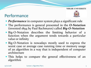
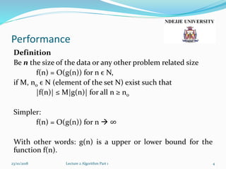
KEMBAR78
Lecture2a algorithm | PPTX
Lecture 2
Algorithm Part 1
23/10/2018 Lecture 2 Algorithm Part 1 1
Content Lecture 2 Part 1
 Performance
 Introduction
 Recursive
 Examples
 Recursion vs. Iteration
 Primitive Recursion Function
 Peano-Hilbert Curve
 Turtle Graphics
23/10/2018 Lecture 2 Algorithm Part 1 2
Performance
 Performance in computer system plays a significant rule
 The performance is general presented in the O-Notation
(invented 1894 by Paul Bachmann) called Big-O-Notation
 Big-O-Notation describes the limiting behavior of a
function when the argument tends towards a particular
value or infinity
 Big-O-Notation is nowadays mostly used to express the
worst case or average case running time or memory usage
of an algorithm in a way that is independent of computer
architecture
 This helps to compare the general effectiveness of an
algorithm
23/10/2018 Lecture 2 Algorithm Part 1 3
Performance
Definition
Be n the size of the data or any other problem related size
f(n) = O(g(n)) for n ϵ N,
if M, n0 ϵ N (element of the set N) exist such that
|f(n)| ≤ M|g(n)| for all n ≥ n0
Simpler:
f(n) = O(g(n)) for n  ∞
With other words: g(n) is a upper or lower bound for the
function f(n).
23/10/2018 Lecture 2 Algorithm Part 1 4
Performance
 The formal definition of Big-O-Notation is not used
directly
 The Big-O-Notation for a function f(x) is derived by the
following rules:
 If f(x) is a sum of several terms the one with the largest
growth rate is kept and all others are ignored
 If f(x) is a product of several factors, any constants
(independent of x) are ignored
23/10/2018 Lecture 2 Algorithm Part 1 5
Performance
Example
f(x) = 7x3 – 3x2 + 11
The function is the sum of three terms: 7x3, -3x2, 11
The one with the largest growth rate it the one with the
largest exponent: 7x3
This term is a product of 7 and x3
Because the factor 7 doesn’t depend on x it can be ignored
As a result you got: f(x) = O(g(x)) = O(x3) with g(x) = x3
23/10/2018 Lecture 2 Algorithm Part 1 6
Performance
List of standard Big-O Notations for comparing algorithm:
O(1)
Constant effort, independent from n
O(n)
Linear effort
23/10/2018 Lecture 2 Algorithm Part 1 7
Performance
O(n log(n))
Effort of good sort methods
O(n2)
Quadratic effort
23/10/2018 Lecture 2 Algorithm Part 1 8
Performance
O(n
k
)
Polynomial effort (with fixed k)
O(2
U
)
Exponential effort
23/10/2018 Lecture 2 Algorithm Part 1 9
Performance
O(n!)
All permutation of n elements
Worst case!
23/10/2018 Lecture 2 Algorithm Part 1 10
Performance
Other performance notations
 theta
 sigma
 small-o
23/10/2018 Lecture 2 Algorithm Part 1 11
Algorithm
What is an algorithm?
23/10/2018 Lecture 2 Algorithm Part 1 12
Algorithm
 A set of instructions done sequentially
 A list of well-defined instructions to complete a given task
 To perform a specified task in a specific order
 It is an effective method to solve a problem expressed as a
finite sequence of steps
 It is not limited to finite (nondeterministic algorithm)
 In computer systems an algorithm is defined as an instance
of logic written in software in order to intend the computer
machine to do something
23/10/2018 Lecture 2 Algorithm Part 1 13
Algorithm
 It is important to define the algorithm rigorously that
means that all possible circumstances for the given task
should be handled
 There is an initial state
 The introductions are done as a series of steps
 The criteria for each step must be clear and computable
 The order of the steps performed is always critical to the
algorithm
 The flow of control is from the top to the bottom (top-
down) that means from a start state to an end state
 Termination might be given to the algorithm but some
algorithm could also run forever without termination
23/10/2018 Lecture 2 Algorithm Part 1 14
Algorithm
 All algorithms are classified in 6 classes:
 Recursion vs. Iteration
 Logical
 Serial(Sequential)/Parallel/Distributed
 Deterministic/Non-deterministic
 Exact/Approximate
 Quantum
23/10/2018 Lecture 2 Algorithm Part 1 15
Algorithm
Recursion vs. Iteration
 Recursive algorithm makes references to itself repeatedly until a
finale state is reached
 Iterative algorithms use repetitive constructs like loops and
sometimes additional data structures
 More details later
Logical
 Algorithm = logic + control
 The logic component defines the axioms that are used in the
computation, the control components determines the way in
which deduction is applied to the axioms
 Example The programming language Prolog
23/10/2018 Lecture 2 Algorithm Part 1 16
Algorithm
Serial(Sequential)/Parallel/Distributed
 Serial Algorithm performing tasks serial that means one step by
one step; Each step is a single operation
 Parallel Algorithm performing multiple operations in each step
 Distributed Algorithm performing tasks distributed
 Examples
 Serial: Calculating the sum of n numbers
 Parallel: Network
 Distributed: GUI, E-mail
23/10/2018 Lecture 2 Algorithm Part 1 17
Algorithm
Deterministic/Non-deterministic
 Deterministic algorithm solve the problem with exact decision
at every step
 Non-deterministic solve problem by guessing through the use
of heuristics
 Example Shopping List
 Buy all items in any order  nondeterministic algorithm
 Buy all items in a given order  deterministic algorithm
Exact/Approximate
 Exact algorithms reach an exact solution
 Approximation algorithms searching for an approximation
close to the true solution
23/10/2018 Lecture 2 Algorithm Part 1 18
Algorithm
 Example: To find an approximate solutions to optimization
problems like storehouses for shops
Quantum
 Quantum algorithm running on a realistic model of quantum
computation
 It is a step-by-step procedure, where each of the steps can be
performed on a quantum computer
 It might be able to solve some problems faster than classical
algorithms
 Example: Shor's algorithm for integer factorization
23/10/2018 Lecture 2 Algorithm Part 1 19
Recursion
 Many problems, models and phenomenon have a self-reflecting
form in which the own structure is contained in different
variants
 This can be a mathematical formula as well as a natural
phenomenon
 If this structure is adopted in a mathematical definition, an
algorithm or a data structure than this is called a recursion
23/10/2018 Lecture 2 Algorithm Part 1 20
Recursion
Definition
Recursion is the process of repeating items in a self-similar way.
 Recursion definitions are only reasonable if something is only
defined by himself in a simpler form
 The limit will be a trivial case
 This case needs no recursion anymore
 A common joke is the following "definition" of recursion
(Catb.org. Retrieved 2010-04-07.):
Recursion
See "Recursion"
23/10/2018 Lecture 2 Algorithm Part 1 21
Recursion
Examples
Language
A child couldn't sleep, so her mother told a story about a little frog,
who couldn't sleep, so the frog's mother told a story about a little bear,
who couldn't sleep, so bear's mother told a story about a little weasel
...who fell asleep.
...and the little bear fell asleep;
...and the little frog fell asleep;
...and the child fell asleep.
23/10/2018 Lecture 2 Algorithm Part 1 22
Mathematical examples
Factorial
 The Factorial of a number if defined as n! = n*(n-1)*(n-2)*…*1
 Therefore:
F(n) = n! for n > 0 is defined: F(1) = 1
F(n) = n * F(n-1) for n > 1
 Program code in C/C++
int factorial(int number) {
if (number <= 1) //trivial case
return number;
return number * (factorial(number - 1)); //recursive call
}
23/10/2018 Lecture 2 Algorithm Part 1 23
Mathematical examples
Calculate F(5) = 5! = 120
23/10/2018 Lecture 2 Algorithm Part 1 24
Recursion
 Because of recursion it is possible that more than one
incarnation of the procedure exists at one time
 It is important that there is finiteness in the recursion (a
trivial case)
 For example a query decided if there is another recursion
call or not
 Otherwise you will have an endless recursive algorithm
calling itself again and again
 In the example it was the case that number <= 1
23/10/2018 Lecture 2 Algorithm Part 1 25
Recursion
Definition
The depth of a recursion is the number of recursion calls.
Example
For factorial the depth of F(n) is n.
depth(F(n)) = n
Because in every step you call the recursion only one time.
Therefore depth(F(5)) = 5
23/10/2018 Lecture 2 Algorithm Part 1 26
Recursion
 There are two ways to implement a recursion:
 Starting from an initial state and deriving new states
which every use of the recursion rules
 Starting from a complex state and simplifying successive
through using the recursion rules until a trivial state is
reached which needs no use of recursion (see Faculty)
 How to build a recursion depends mainly on:
 How readable and understandable the alternative
variants are
 Performance and memory issues
23/10/2018 Lecture 2 Algorithm Part 1 27
Mathematical examples
Greatest Common Divisor
 The Greatest Common Divisor gcd(x,y) of the integer x
and y s is the product of all common prime number factors
of x and y
 To calculate the gcd you can use the following formula:
gcd(x1, y1) = gcd(y1, x1 % y1) =gcd(x2, y2) =
= gcd(y2, x2 % y2) = … = gcd(xk, 0)
 The final gcd(xk, 0) = xk is the Greatest common divisor
23/10/2018 Lecture 2 Algorithm Part 1 28
Mathematical examples
Implementation in C
int mygcd(int x, int y) {
if (y == 0) //trivial case
return x;
else
return mygcd(y, x % y); //recursive call
}
gcd(34, 16) = gcd(16, 2) = gcd(2, 0) = 2
gcd(127, 36)=gcd(36, 19)=gcd(19, 17)=gcd(17, 2)=gcd(2, 1)=gcd(1, 0)=1
23/10/2018 Lecture 2 Algorithm Part 1 29
Mathematical examples
Fibonacci sequence
 Fibonacci sequence is one of the classical example of
recursion
 Leonardo Fibonacci was an Italian mathematician (around
1180 – 1240)
 The Fibonacci sequence can be found also in nature
(plants)
 The sequence is defined as:
 F(0) = 0 (base case)
 F(1) = 1 (base case)
 F(n) = F(n-1) + F(n-2) (recursion) for all n > 1 with n ϵ N
23/10/2018 Lecture 2 Algorithm Part 1 30
Mathematical examples
Calculate F(4) = 3
23/10/2018 Lecture 2 Algorithm Part 1 31
Mathematical examples
Ackermann function
 Wilhelm Ackermann was a German mathematician (1896 –
1962)
 The Ackermann function is used as a benchmark of the
ability of a compiler to optimize recursion
 The function is defined as:
𝐴 𝑚, 𝑛 =
𝑛 + 1 𝑖𝑓 𝑚 = 0
𝐴 𝑚 − 1, 1 𝑖𝑓 𝑚 > 0 𝑎𝑛𝑑 𝑛 = 0
𝐴 𝑚 − 1, 𝐴 𝑚, 𝑛 − 1 𝑖𝑓 𝑚 > 0 𝑎𝑛𝑑 𝑛 > 0
23/10/2018 Lecture 2 Algorithm Part 1 32
Mathematical examples
Implementation in C
int ackermann(int m, int n) {
if (m == 0) //trivial case
return n + 1;
else if (n == 0) //recursive call
return ackermann(m – 1, 1);
else //recursive call
return ackermann(m – 1, ackermann(m, n – 1));
}
23/10/2018 Lecture 2 Algorithm Part 1 33
Recursion vs. Iteration
 Use of recursion in an algorithm has both advantages and
disadvantages
 The main advantage is usually simplicity
 The main disadvantage is often that the algorithm may require
large amounts of memory if the depth of the recursion is very
high
 Many problems are solved more elegant and efficient if they are
implemented by using iteration
 This is especially the case for tail recursions which can be
replaced immediately by a loop, because no nested case exists
which has to be represented by a recursion
 The recursive call happens only at the end of the algorithm
 Recursion and iteration are not really contrasts because every
recursion can also be implemented as iteration
23/10/2018 Lecture 2 Algorithm Part 1 34
Recursion vs. Iteration
Tail recursion
int tail_recursion(…) {
if (simple_case) //trivial case
/*do something */;
else
/*do something */;
tail_recursion(…); // only recursive call
}
23/10/2018 Lecture 2 Algorithm Part 1 35
Recursion vs. Iteration
Examples
 The factorial algorithm is more efficient if you use an iterative
implementation
int factorial_iterative(int number) {
int result = 1;
while (number > 0) {
result *= number;
number--;
}
return number;
}
 Whereas the Ackermann function is an example where it is more
efficient and simpler to implement it with recursion
23/10/2018 Lecture 2 Algorithm Part 1 36
Primitive Recursion Function
Definition
The primitive recursive functions are among the number-
theoretic functions, which are functions from the natural
numbers (non negative integers) {0, 1, 2 , ...} to the natural
numbers
 These functions take n arguments for some natural
number n and are called n-ary
 Functions in number theory are primitive recursive
 Important also in proof theory (proof by induction)
23/10/2018 Lecture 2 Algorithm Part 1 37
Primitive Recursion Function
 The basic primitive recursive functions are given by these
axioms:
 Constant function: The 0-ary constant function 0 is
primitive recursive
 Successor function: The 1-ary successor function S,
which returns the successor of its argument, is primitive
recursive. That is, S(k) = k + 1
 Projection function: For every n ≥ 1 and each i with 1 ≤
i ≤ n, the n-ary projection function Pi
n, which returns
its ith argument, is primitive recursive
23/10/2018 Lecture 2 Algorithm Part 1 38
Primitive Recursion Function
Examples
 Addition: x + y
 Add(0, x) = x
 Add(y + 1, x) = Add(y, x) + 1
 Multiplication: x*y
 Exponentiation: xy,
 Factorial: n!
 Minimum: (n1, ... nn)
 Maximum: (n1, ... nn)
23/10/2018 Lecture 2 Algorithm Part 1 39
Peano-Hilbert curve
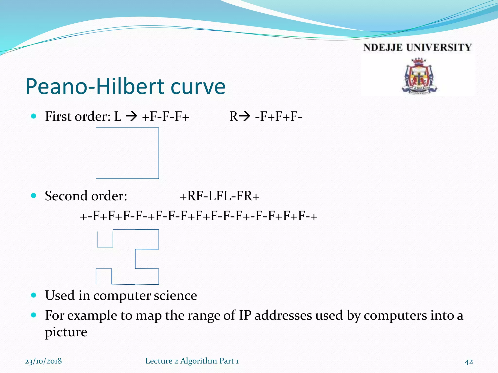
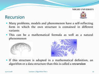
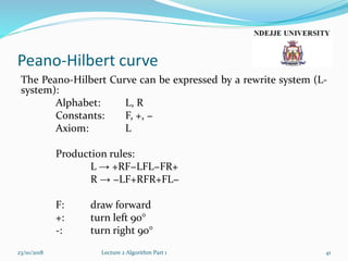
 The Peano-Hilbert curves were discovered by Peano and
Hilbert in 1890/1891
 They convert against a function which maps the interval
[0,1] of the real numbers surjective on the area [0,1] x [0,1]
and is in the same time constant
 That means through repeatedly execute the function rules
you will reach every point in a square
23/10/2018 Lecture 2 Algorithm Part 1 40
Peano-Hilbert curve
The Peano-Hilbert Curve can be expressed by a rewrite system (L-
system):
Alphabet: L, R
Constants: F, +, −
Axiom: L
Production rules:
L → +RF−LFL−FR+
R → −LF+RFR+FL−
F: draw forward
+: turn left 90°
-: turn right 90°
23/10/2018 Lecture 2 Algorithm Part 1 41
Peano-Hilbert curve
 First order: L  +F-F-F+ R -F+F+F-
 Second order: +RF-LFL-FR+
+-F+F+F-F-+F-F-F+F+F-F-F+-F-F+F+F-+
 Used in computer science
 For example to map the range of IP addresses used by computers into a
picture
23/10/2018 Lecture 2 Algorithm Part 1 42
Turtle Graphics
 Turtle Graphics are connected to the program language Logo
(1967)
 There is no absolute position in a coordination system
 All introductions are relative to the actual position
 A simple form would be:
Alphabet: X, Y
Constants: F, +, −
Production rules:
Initial Value: FX
X → X+YF+
Y → -FX-Y
23/10/2018 Lecture 2 Algorithm Part 1 43
F: draw forward
+: turn left 90°
-: turn right 90°
Turtle Graphics
 Level 1: FX = F+F+
 Level 2: FX = FX+YF+ = F+F++-F-F+
23/10/2018 Lecture 2 Algorithm Part 1 44
Turtle Graphics
Other turtle graphic
23/10/2018 Lecture 2 Algorithm Part 1 45
Any
questions?
23/10/2018 Lecture 2 Algorithm Part 1 46

Lecture2a algorithm

  • 1.
    Lecture 2 Algorithm Part1 23/10/2018 Lecture 2 Algorithm Part 1 1
  • 2.
    Content Lecture 2Part 1  Performance  Introduction  Recursive  Examples  Recursion vs. Iteration  Primitive Recursion Function  Peano-Hilbert Curve  Turtle Graphics 23/10/2018 Lecture 2 Algorithm Part 1 2
  • 3.
    Performance  Performance incomputer system plays a significant rule  The performance is general presented in the O-Notation (invented 1894 by Paul Bachmann) called Big-O-Notation  Big-O-Notation describes the limiting behavior of a function when the argument tends towards a particular value or infinity  Big-O-Notation is nowadays mostly used to express the worst case or average case running time or memory usage of an algorithm in a way that is independent of computer architecture  This helps to compare the general effectiveness of an algorithm 23/10/2018 Lecture 2 Algorithm Part 1 3
  • 4.
    Performance Definition Be n thesize of the data or any other problem related size f(n) = O(g(n)) for n ϵ N, if M, n0 ϵ N (element of the set N) exist such that |f(n)| ≤ M|g(n)| for all n ≥ n0 Simpler: f(n) = O(g(n)) for n  ∞ With other words: g(n) is a upper or lower bound for the function f(n). 23/10/2018 Lecture 2 Algorithm Part 1 4
  • 5.
    Performance  The formaldefinition of Big-O-Notation is not used directly  The Big-O-Notation for a function f(x) is derived by the following rules:  If f(x) is a sum of several terms the one with the largest growth rate is kept and all others are ignored  If f(x) is a product of several factors, any constants (independent of x) are ignored 23/10/2018 Lecture 2 Algorithm Part 1 5
  • 6.
    Performance Example f(x) = 7x3– 3x2 + 11 The function is the sum of three terms: 7x3, -3x2, 11 The one with the largest growth rate it the one with the largest exponent: 7x3 This term is a product of 7 and x3 Because the factor 7 doesn’t depend on x it can be ignored As a result you got: f(x) = O(g(x)) = O(x3) with g(x) = x3 23/10/2018 Lecture 2 Algorithm Part 1 6
  • 7.
    Performance List of standardBig-O Notations for comparing algorithm: O(1) Constant effort, independent from n O(n) Linear effort 23/10/2018 Lecture 2 Algorithm Part 1 7
  • 8.
    Performance O(n log(n)) Effort ofgood sort methods O(n2) Quadratic effort 23/10/2018 Lecture 2 Algorithm Part 1 8
  • 9.
    Performance O(n k ) Polynomial effort (withfixed k) O(2 U ) Exponential effort 23/10/2018 Lecture 2 Algorithm Part 1 9
  • 10.
    Performance O(n!) All permutation ofn elements Worst case! 23/10/2018 Lecture 2 Algorithm Part 1 10
  • 11.
    Performance Other performance notations theta  sigma  small-o 23/10/2018 Lecture 2 Algorithm Part 1 11
  • 12.
    Algorithm What is analgorithm? 23/10/2018 Lecture 2 Algorithm Part 1 12
  • 13.
    Algorithm  A setof instructions done sequentially  A list of well-defined instructions to complete a given task  To perform a specified task in a specific order  It is an effective method to solve a problem expressed as a finite sequence of steps  It is not limited to finite (nondeterministic algorithm)  In computer systems an algorithm is defined as an instance of logic written in software in order to intend the computer machine to do something 23/10/2018 Lecture 2 Algorithm Part 1 13
  • 14.
    Algorithm  It isimportant to define the algorithm rigorously that means that all possible circumstances for the given task should be handled  There is an initial state  The introductions are done as a series of steps  The criteria for each step must be clear and computable  The order of the steps performed is always critical to the algorithm  The flow of control is from the top to the bottom (top- down) that means from a start state to an end state  Termination might be given to the algorithm but some algorithm could also run forever without termination 23/10/2018 Lecture 2 Algorithm Part 1 14
  • 15.
    Algorithm  All algorithmsare classified in 6 classes:  Recursion vs. Iteration  Logical  Serial(Sequential)/Parallel/Distributed  Deterministic/Non-deterministic  Exact/Approximate  Quantum 23/10/2018 Lecture 2 Algorithm Part 1 15
  • 16.
    Algorithm Recursion vs. Iteration Recursive algorithm makes references to itself repeatedly until a finale state is reached  Iterative algorithms use repetitive constructs like loops and sometimes additional data structures  More details later Logical  Algorithm = logic + control  The logic component defines the axioms that are used in the computation, the control components determines the way in which deduction is applied to the axioms  Example The programming language Prolog 23/10/2018 Lecture 2 Algorithm Part 1 16
  • 17.
    Algorithm Serial(Sequential)/Parallel/Distributed  Serial Algorithmperforming tasks serial that means one step by one step; Each step is a single operation  Parallel Algorithm performing multiple operations in each step  Distributed Algorithm performing tasks distributed  Examples  Serial: Calculating the sum of n numbers  Parallel: Network  Distributed: GUI, E-mail 23/10/2018 Lecture 2 Algorithm Part 1 17
  • 18.
    Algorithm Deterministic/Non-deterministic  Deterministic algorithmsolve the problem with exact decision at every step  Non-deterministic solve problem by guessing through the use of heuristics  Example Shopping List  Buy all items in any order  nondeterministic algorithm  Buy all items in a given order  deterministic algorithm Exact/Approximate  Exact algorithms reach an exact solution  Approximation algorithms searching for an approximation close to the true solution 23/10/2018 Lecture 2 Algorithm Part 1 18
  • 19.
    Algorithm  Example: Tofind an approximate solutions to optimization problems like storehouses for shops Quantum  Quantum algorithm running on a realistic model of quantum computation  It is a step-by-step procedure, where each of the steps can be performed on a quantum computer  It might be able to solve some problems faster than classical algorithms  Example: Shor's algorithm for integer factorization 23/10/2018 Lecture 2 Algorithm Part 1 19
  • 20.
    Recursion  Many problems,models and phenomenon have a self-reflecting form in which the own structure is contained in different variants  This can be a mathematical formula as well as a natural phenomenon  If this structure is adopted in a mathematical definition, an algorithm or a data structure than this is called a recursion 23/10/2018 Lecture 2 Algorithm Part 1 20
  • 21.
    Recursion Definition Recursion is theprocess of repeating items in a self-similar way.  Recursion definitions are only reasonable if something is only defined by himself in a simpler form  The limit will be a trivial case  This case needs no recursion anymore  A common joke is the following "definition" of recursion (Catb.org. Retrieved 2010-04-07.): Recursion See "Recursion" 23/10/2018 Lecture 2 Algorithm Part 1 21
  • 22.
    Recursion Examples Language A child couldn'tsleep, so her mother told a story about a little frog, who couldn't sleep, so the frog's mother told a story about a little bear, who couldn't sleep, so bear's mother told a story about a little weasel ...who fell asleep. ...and the little bear fell asleep; ...and the little frog fell asleep; ...and the child fell asleep. 23/10/2018 Lecture 2 Algorithm Part 1 22
  • 23.
    Mathematical examples Factorial  TheFactorial of a number if defined as n! = n*(n-1)*(n-2)*…*1  Therefore: F(n) = n! for n > 0 is defined: F(1) = 1 F(n) = n * F(n-1) for n > 1  Program code in C/C++ int factorial(int number) { if (number <= 1) //trivial case return number; return number * (factorial(number - 1)); //recursive call } 23/10/2018 Lecture 2 Algorithm Part 1 23
  • 24.
    Mathematical examples Calculate F(5)= 5! = 120 23/10/2018 Lecture 2 Algorithm Part 1 24
  • 25.
    Recursion  Because ofrecursion it is possible that more than one incarnation of the procedure exists at one time  It is important that there is finiteness in the recursion (a trivial case)  For example a query decided if there is another recursion call or not  Otherwise you will have an endless recursive algorithm calling itself again and again  In the example it was the case that number <= 1 23/10/2018 Lecture 2 Algorithm Part 1 25
  • 26.
    Recursion Definition The depth ofa recursion is the number of recursion calls. Example For factorial the depth of F(n) is n. depth(F(n)) = n Because in every step you call the recursion only one time. Therefore depth(F(5)) = 5 23/10/2018 Lecture 2 Algorithm Part 1 26
  • 27.
    Recursion  There aretwo ways to implement a recursion:  Starting from an initial state and deriving new states which every use of the recursion rules  Starting from a complex state and simplifying successive through using the recursion rules until a trivial state is reached which needs no use of recursion (see Faculty)  How to build a recursion depends mainly on:  How readable and understandable the alternative variants are  Performance and memory issues 23/10/2018 Lecture 2 Algorithm Part 1 27
  • 28.
    Mathematical examples Greatest CommonDivisor  The Greatest Common Divisor gcd(x,y) of the integer x and y s is the product of all common prime number factors of x and y  To calculate the gcd you can use the following formula: gcd(x1, y1) = gcd(y1, x1 % y1) =gcd(x2, y2) = = gcd(y2, x2 % y2) = … = gcd(xk, 0)  The final gcd(xk, 0) = xk is the Greatest common divisor 23/10/2018 Lecture 2 Algorithm Part 1 28
  • 29.
    Mathematical examples Implementation inC int mygcd(int x, int y) { if (y == 0) //trivial case return x; else return mygcd(y, x % y); //recursive call } gcd(34, 16) = gcd(16, 2) = gcd(2, 0) = 2 gcd(127, 36)=gcd(36, 19)=gcd(19, 17)=gcd(17, 2)=gcd(2, 1)=gcd(1, 0)=1 23/10/2018 Lecture 2 Algorithm Part 1 29
  • 30.
    Mathematical examples Fibonacci sequence Fibonacci sequence is one of the classical example of recursion  Leonardo Fibonacci was an Italian mathematician (around 1180 – 1240)  The Fibonacci sequence can be found also in nature (plants)  The sequence is defined as:  F(0) = 0 (base case)  F(1) = 1 (base case)  F(n) = F(n-1) + F(n-2) (recursion) for all n > 1 with n ϵ N 23/10/2018 Lecture 2 Algorithm Part 1 30
  • 31.
    Mathematical examples Calculate F(4)= 3 23/10/2018 Lecture 2 Algorithm Part 1 31
  • 32.
    Mathematical examples Ackermann function Wilhelm Ackermann was a German mathematician (1896 – 1962)  The Ackermann function is used as a benchmark of the ability of a compiler to optimize recursion  The function is defined as: 𝐴 𝑚, 𝑛 = 𝑛 + 1 𝑖𝑓 𝑚 = 0 𝐴 𝑚 − 1, 1 𝑖𝑓 𝑚 > 0 𝑎𝑛𝑑 𝑛 = 0 𝐴 𝑚 − 1, 𝐴 𝑚, 𝑛 − 1 𝑖𝑓 𝑚 > 0 𝑎𝑛𝑑 𝑛 > 0 23/10/2018 Lecture 2 Algorithm Part 1 32
  • 33.
    Mathematical examples Implementation inC int ackermann(int m, int n) { if (m == 0) //trivial case return n + 1; else if (n == 0) //recursive call return ackermann(m – 1, 1); else //recursive call return ackermann(m – 1, ackermann(m, n – 1)); } 23/10/2018 Lecture 2 Algorithm Part 1 33
  • 34.
    Recursion vs. Iteration Use of recursion in an algorithm has both advantages and disadvantages  The main advantage is usually simplicity  The main disadvantage is often that the algorithm may require large amounts of memory if the depth of the recursion is very high  Many problems are solved more elegant and efficient if they are implemented by using iteration  This is especially the case for tail recursions which can be replaced immediately by a loop, because no nested case exists which has to be represented by a recursion  The recursive call happens only at the end of the algorithm  Recursion and iteration are not really contrasts because every recursion can also be implemented as iteration 23/10/2018 Lecture 2 Algorithm Part 1 34
  • 35.
    Recursion vs. Iteration Tailrecursion int tail_recursion(…) { if (simple_case) //trivial case /*do something */; else /*do something */; tail_recursion(…); // only recursive call } 23/10/2018 Lecture 2 Algorithm Part 1 35
  • 36.
    Recursion vs. Iteration Examples The factorial algorithm is more efficient if you use an iterative implementation int factorial_iterative(int number) { int result = 1; while (number > 0) { result *= number; number--; } return number; }  Whereas the Ackermann function is an example where it is more efficient and simpler to implement it with recursion 23/10/2018 Lecture 2 Algorithm Part 1 36
  • 37.
    Primitive Recursion Function Definition Theprimitive recursive functions are among the number- theoretic functions, which are functions from the natural numbers (non negative integers) {0, 1, 2 , ...} to the natural numbers  These functions take n arguments for some natural number n and are called n-ary  Functions in number theory are primitive recursive  Important also in proof theory (proof by induction) 23/10/2018 Lecture 2 Algorithm Part 1 37
  • 38.
    Primitive Recursion Function The basic primitive recursive functions are given by these axioms:  Constant function: The 0-ary constant function 0 is primitive recursive  Successor function: The 1-ary successor function S, which returns the successor of its argument, is primitive recursive. That is, S(k) = k + 1  Projection function: For every n ≥ 1 and each i with 1 ≤ i ≤ n, the n-ary projection function Pi n, which returns its ith argument, is primitive recursive 23/10/2018 Lecture 2 Algorithm Part 1 38
  • 39.
    Primitive Recursion Function Examples Addition: x + y  Add(0, x) = x  Add(y + 1, x) = Add(y, x) + 1  Multiplication: x*y  Exponentiation: xy,  Factorial: n!  Minimum: (n1, ... nn)  Maximum: (n1, ... nn) 23/10/2018 Lecture 2 Algorithm Part 1 39
  • 40.
    Peano-Hilbert curve  ThePeano-Hilbert curves were discovered by Peano and Hilbert in 1890/1891  They convert against a function which maps the interval [0,1] of the real numbers surjective on the area [0,1] x [0,1] and is in the same time constant  That means through repeatedly execute the function rules you will reach every point in a square 23/10/2018 Lecture 2 Algorithm Part 1 40
  • 41.
    Peano-Hilbert curve The Peano-HilbertCurve can be expressed by a rewrite system (L- system): Alphabet: L, R Constants: F, +, − Axiom: L Production rules: L → +RF−LFL−FR+ R → −LF+RFR+FL− F: draw forward +: turn left 90° -: turn right 90° 23/10/2018 Lecture 2 Algorithm Part 1 41
  • 42.
    Peano-Hilbert curve  Firstorder: L  +F-F-F+ R -F+F+F-  Second order: +RF-LFL-FR+ +-F+F+F-F-+F-F-F+F+F-F-F+-F-F+F+F-+  Used in computer science  For example to map the range of IP addresses used by computers into a picture 23/10/2018 Lecture 2 Algorithm Part 1 42
  • 43.
    Turtle Graphics  TurtleGraphics are connected to the program language Logo (1967)  There is no absolute position in a coordination system  All introductions are relative to the actual position  A simple form would be: Alphabet: X, Y Constants: F, +, − Production rules: Initial Value: FX X → X+YF+ Y → -FX-Y 23/10/2018 Lecture 2 Algorithm Part 1 43 F: draw forward +: turn left 90° -: turn right 90°
  • 44.
    Turtle Graphics  Level1: FX = F+F+  Level 2: FX = FX+YF+ = F+F++-F-F+ 23/10/2018 Lecture 2 Algorithm Part 1 44
  • 45.
    Turtle Graphics Other turtlegraphic 23/10/2018 Lecture 2 Algorithm Part 1 45
  • 46.

Editor's Notes

  • #5 Betragsfunktion = Absolute value function
  • #17 Axiom = something that I just true – no proof
  • #41 For each y exist an x with f(x) = x