Downloaded 102 times

![Sorting In Linear Time
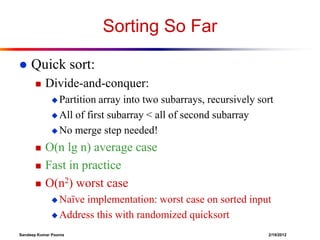
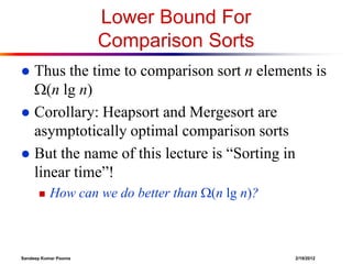
Counting sort
No comparisons between elements!
But…depends on assumption about the numbers
being sorted
We
assume numbers are in the range 1.. k
The algorithm:
A[1..n], where A[j] {1, 2, 3, …, k}
Output: B[1..n], sorted (notice: not sorting in place)
Also: Array C[1..k] for auxiliary storage
Input:
Sandeep Kumar Poonia
2/19/2012](https://image.slidesharecdn.com/linear-timesortingalgorithms-140217061848-phpapp02/85/Linear-time-sorting-algorithms-15-320.jpg)
![Counting Sort
1
2
3
4
5
6
7
8
9
10
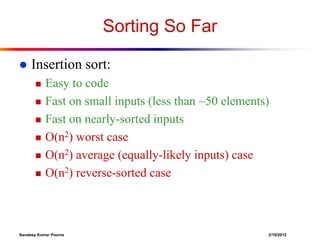
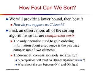
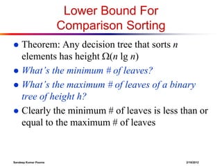
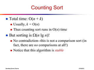
CountingSort(A, B, k)
for i=0 to k
C[i]= 0;
for j=1 to n
C[A[j]]= C[A[j]] + 1;
for i=2 to k
C[i] = C[i] + C[i-1];
for j=n downto 1
B[C[A[j]]] = A[j];
C[A[j]] = C[A[j]] - 1;
Sandeep Kumar Poonia
2/19/2012](https://image.slidesharecdn.com/linear-timesortingalgorithms-140217061848-phpapp02/85/Linear-time-sorting-algorithms-16-320.jpg)
![Counting Sort
1
2
3
4
5
6
7
8
9
10
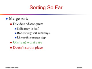
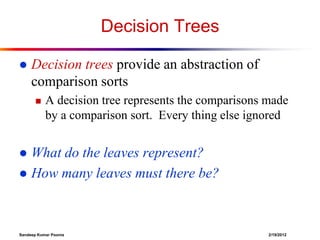
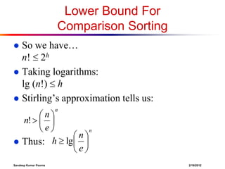
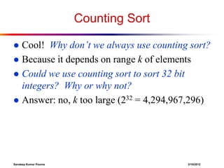
CountingSort(A, B, k)
for i=1 to k
Takes time O(k)
C[i]= 0;
for j=1 to n
C[A[j]] += 1;
for i=2 to k
C[i] = C[i] + C[i-1];
Takes time O(n)
for j=n downto 1
B[C[A[j]]] = A[j];
C[A[j]] -= 1;
What will be the running time?
Sandeep Kumar Poonia
2/19/2012](https://image.slidesharecdn.com/linear-timesortingalgorithms-140217061848-phpapp02/85/Linear-time-sorting-algorithms-17-320.jpg)


![Sorting In Linear Time
Counting sort
No comparisons between elements!
But…depends on assumption about the numbers
being sorted
We
assume numbers are in the range 1.. k
The algorithm:
A[1..n], where A[j] {1, 2, 3, …, k}
Output: B[1..n], sorted (notice: not sorting in place)
Also: Array C[1..k] for auxiliary storage
Input:
Sandeep Kumar Poonia
2/19/2012](https://image.slidesharecdn.com/linear-timesortingalgorithms-140217061848-phpapp02/75/Linear-time-sorting-algorithms-15-2048.jpg)
![Counting Sort
1
2
3
4
5
6
7
8
9
10
CountingSort(A, B, k)
for i=0 to k
C[i]= 0;
for j=1 to n
C[A[j]]= C[A[j]] + 1;
for i=2 to k
C[i] = C[i] + C[i-1];
for j=n downto 1
B[C[A[j]]] = A[j];
C[A[j]] = C[A[j]] - 1;
Sandeep Kumar Poonia
2/19/2012](https://image.slidesharecdn.com/linear-timesortingalgorithms-140217061848-phpapp02/75/Linear-time-sorting-algorithms-16-2048.jpg)
![Counting Sort
1
2
3
4
5
6
7
8
9
10
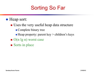
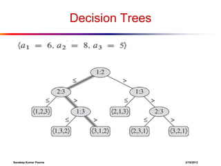
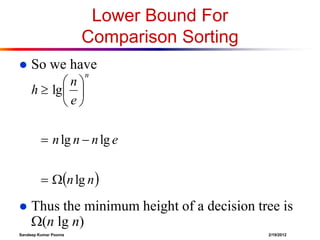
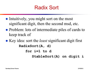
CountingSort(A, B, k)
for i=1 to k
Takes time O(k)
C[i]= 0;
for j=1 to n
C[A[j]] += 1;
for i=2 to k
C[i] = C[i] + C[i-1];
Takes time O(n)
for j=n downto 1
B[C[A[j]]] = A[j];
C[A[j]] -= 1;
What will be the running time?
Sandeep Kumar Poonia
2/19/2012](https://image.slidesharecdn.com/linear-timesortingalgorithms-140217061848-phpapp02/75/Linear-time-sorting-algorithms-17-2048.jpg)
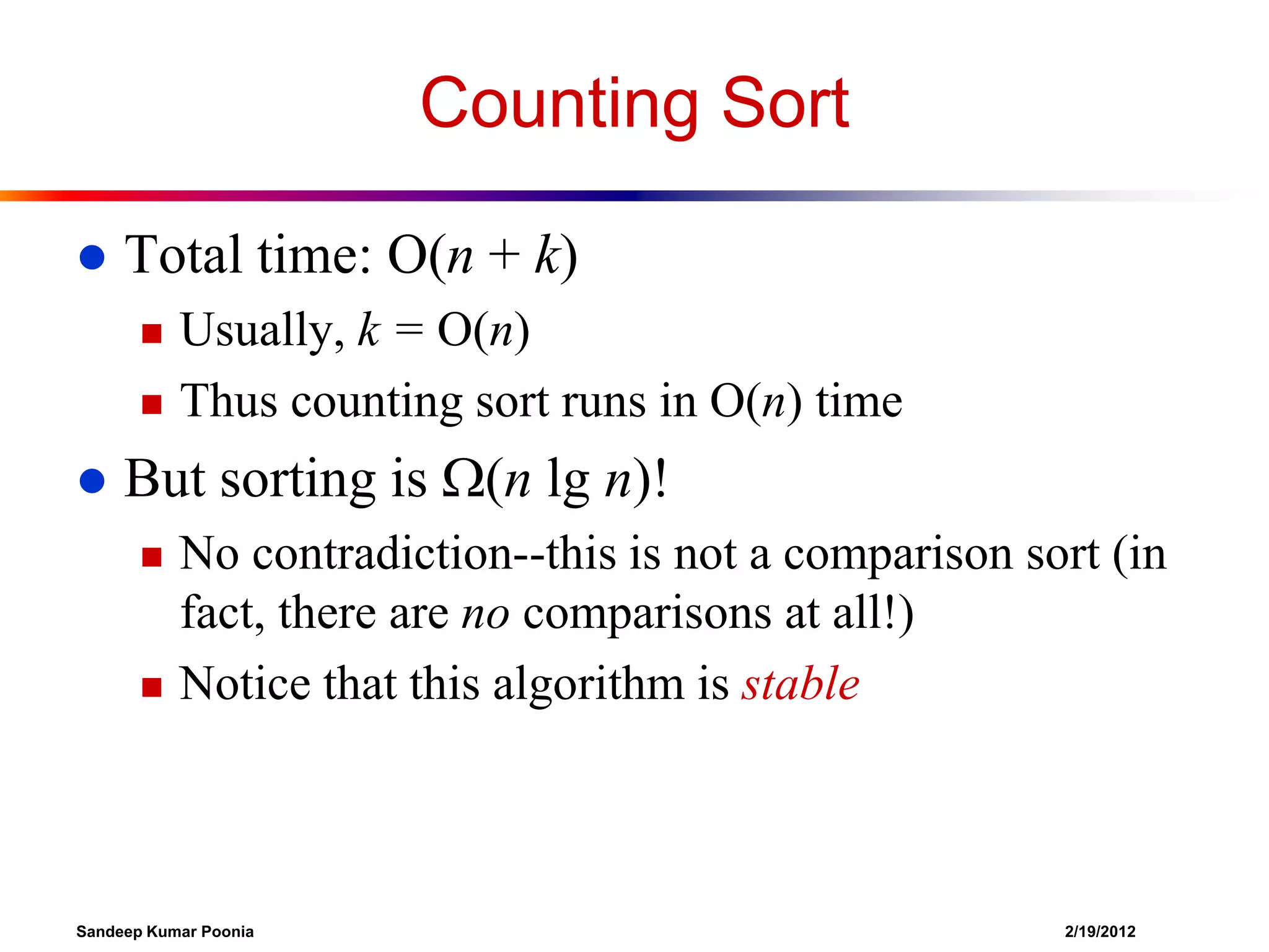
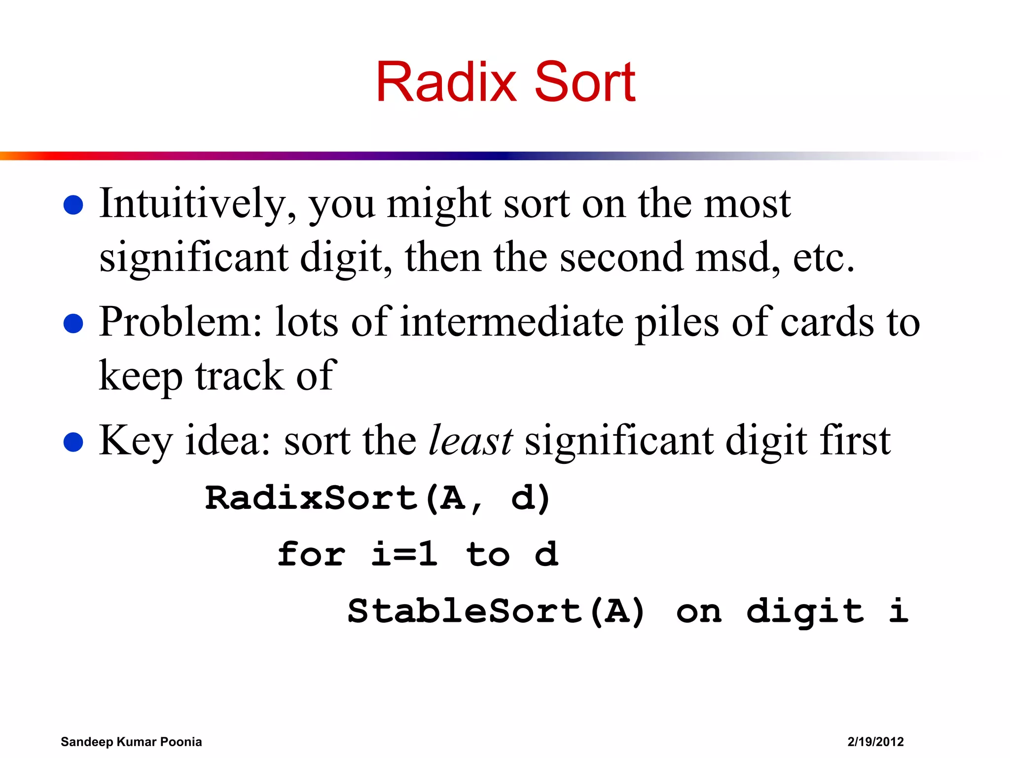
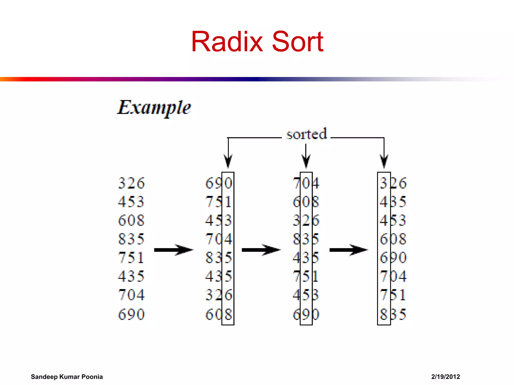
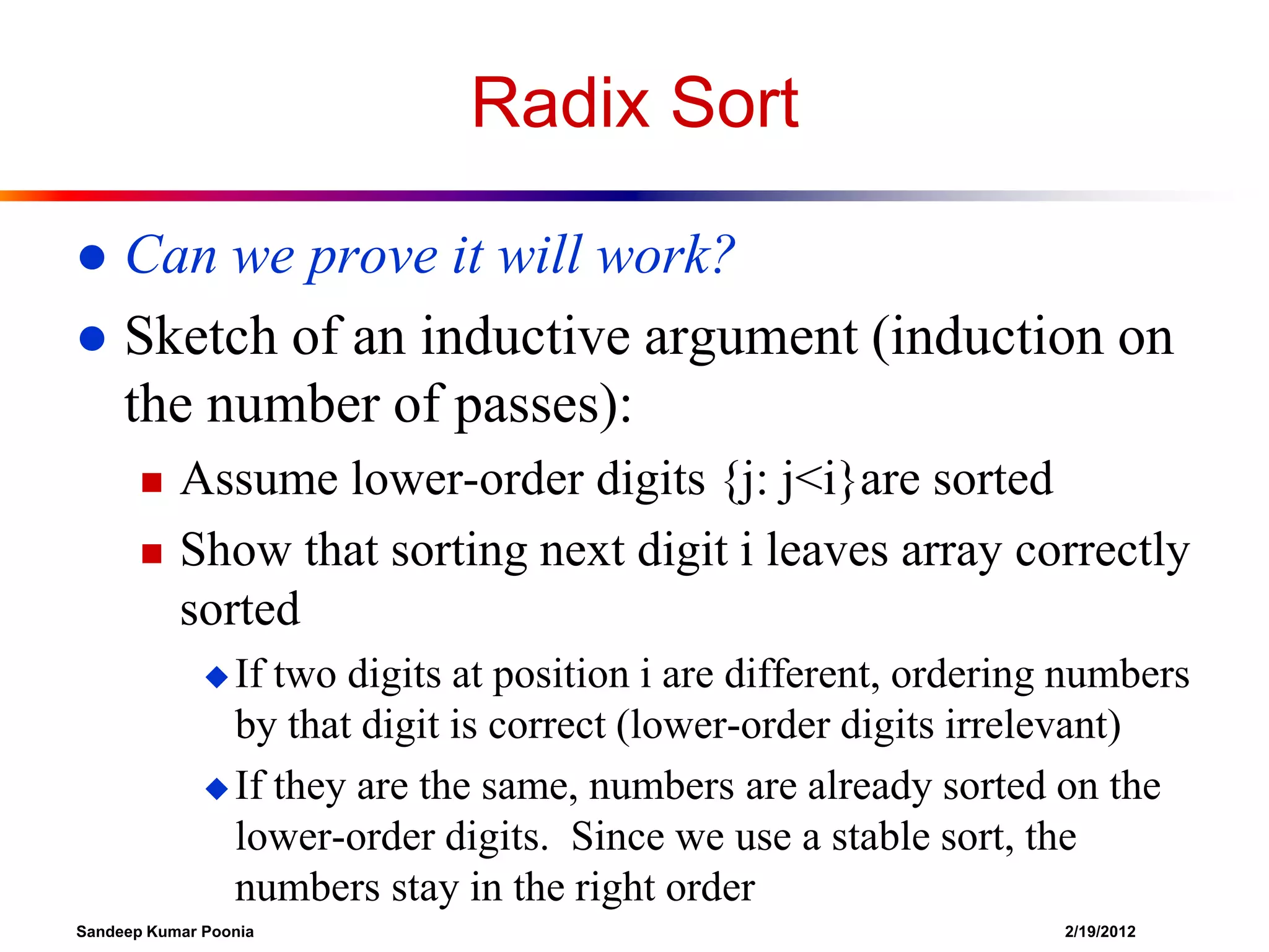
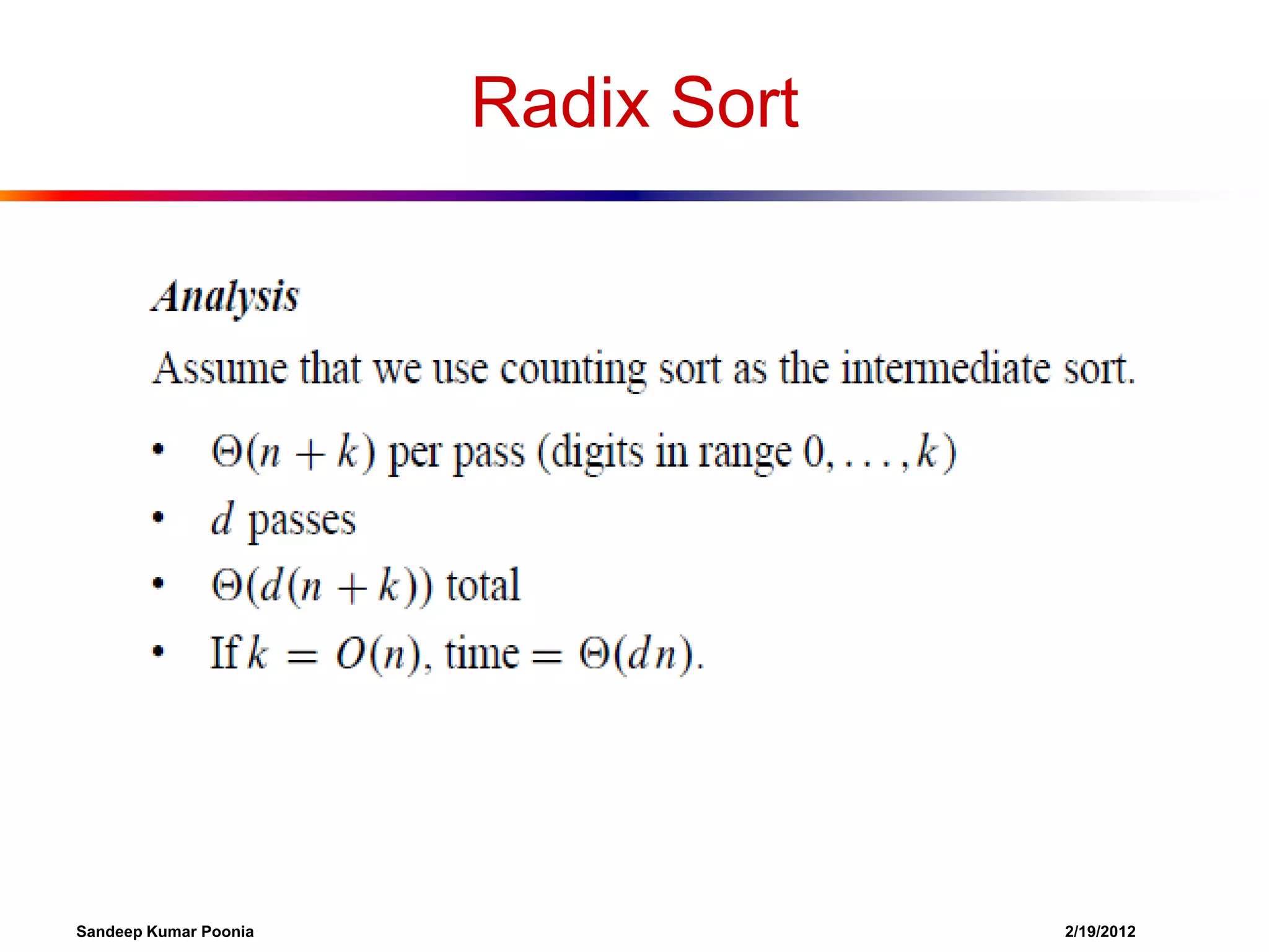
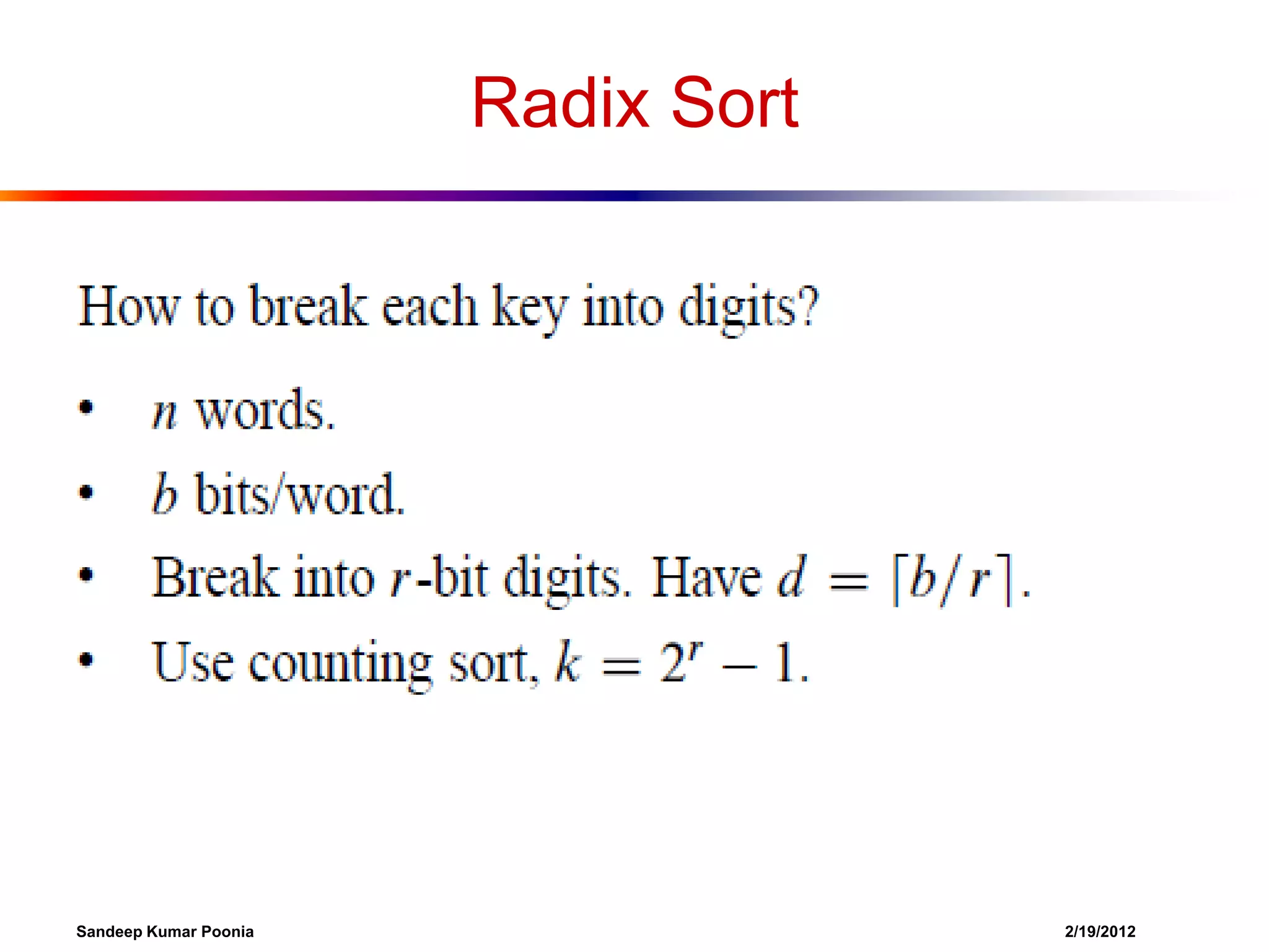
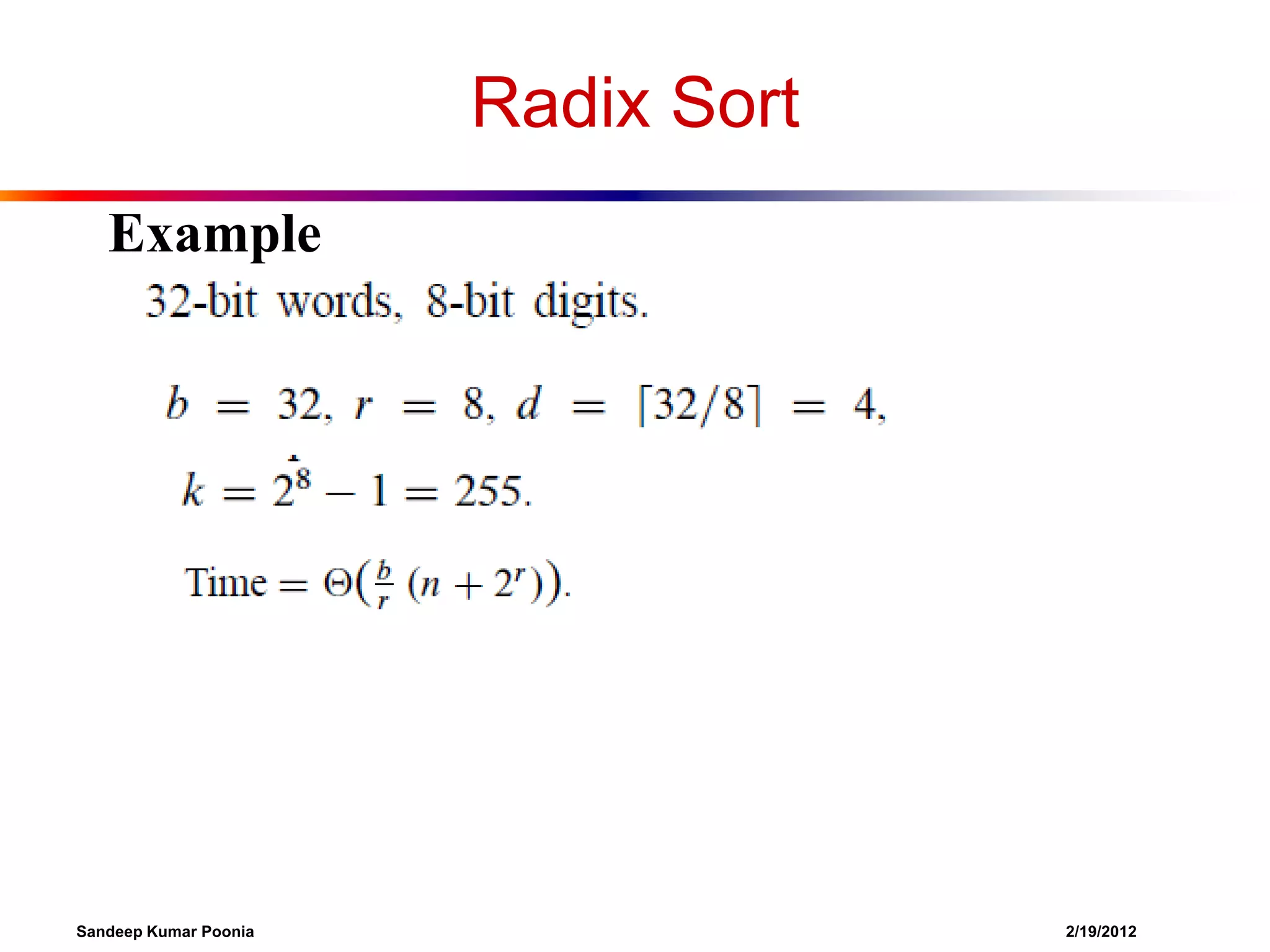
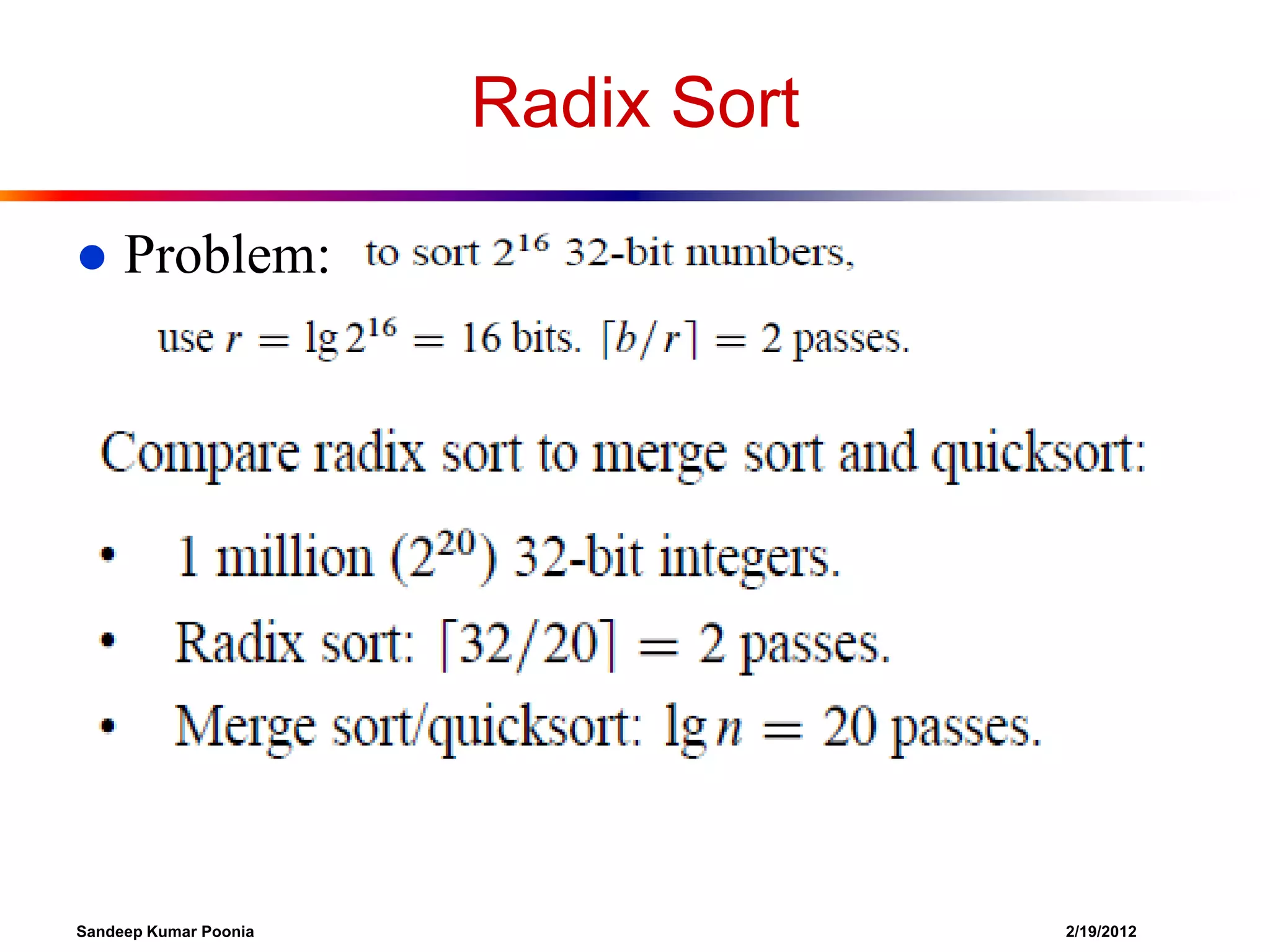
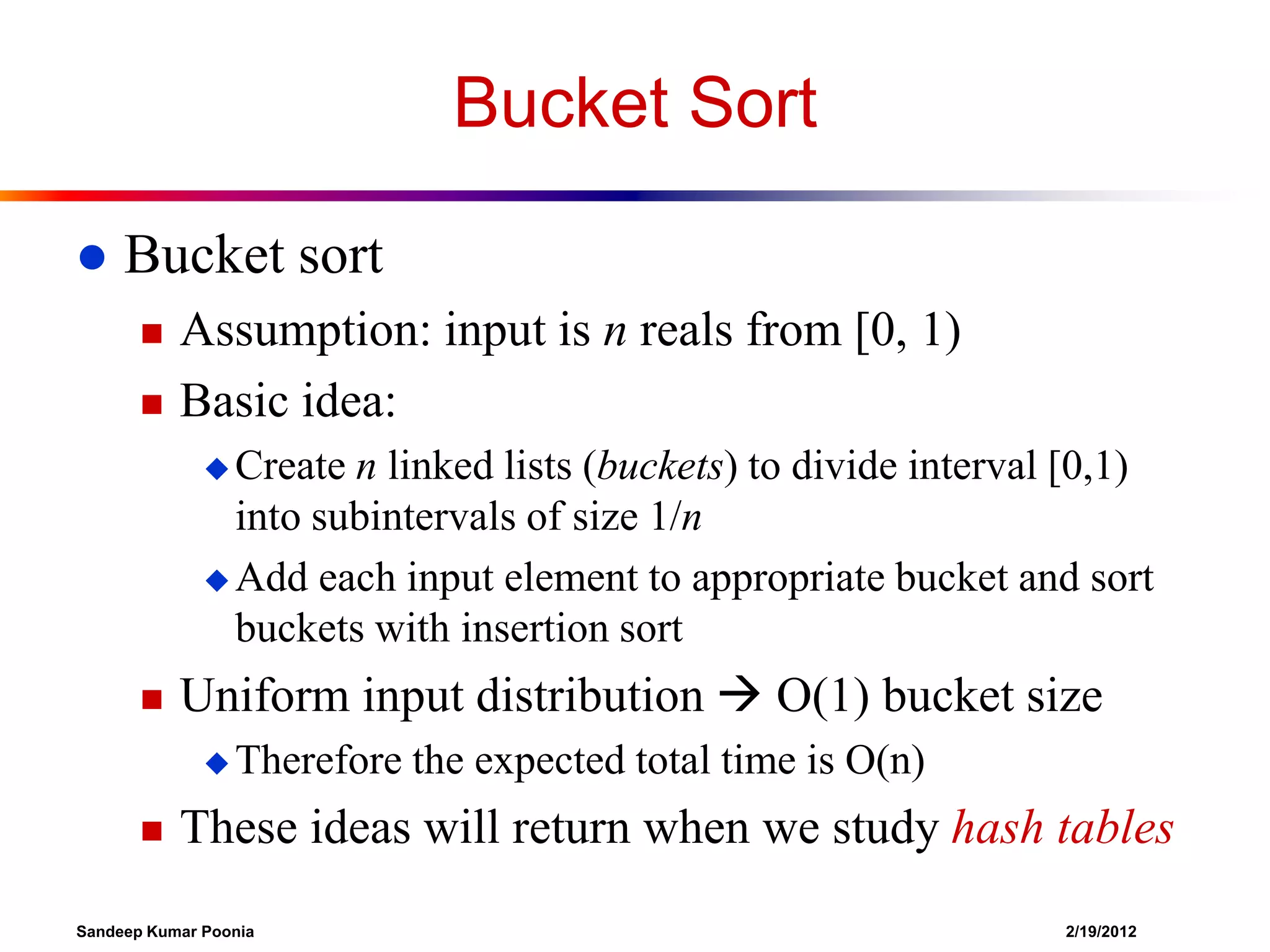
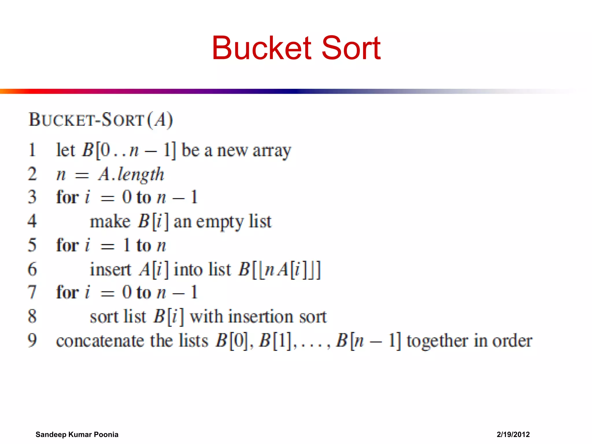
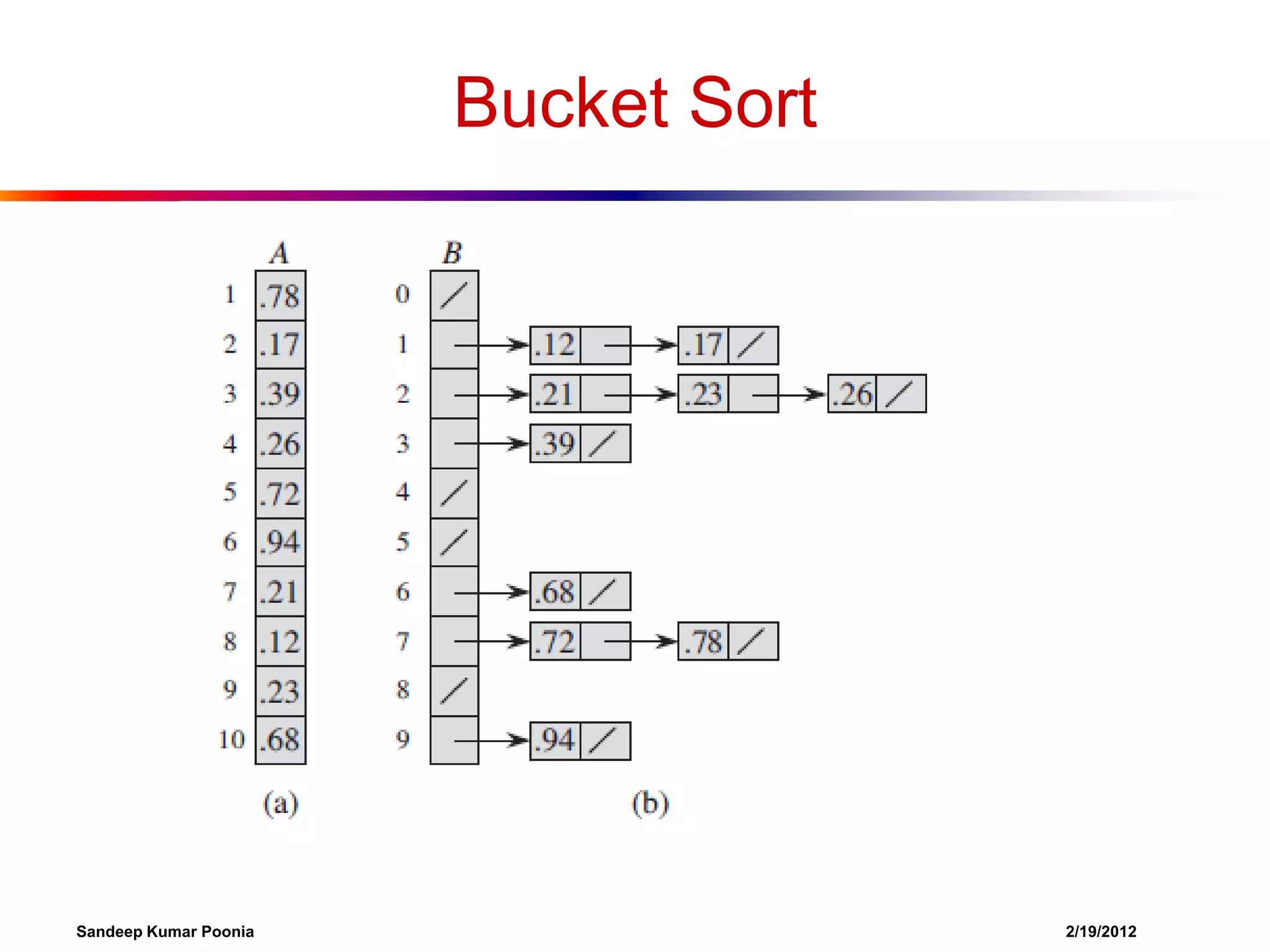
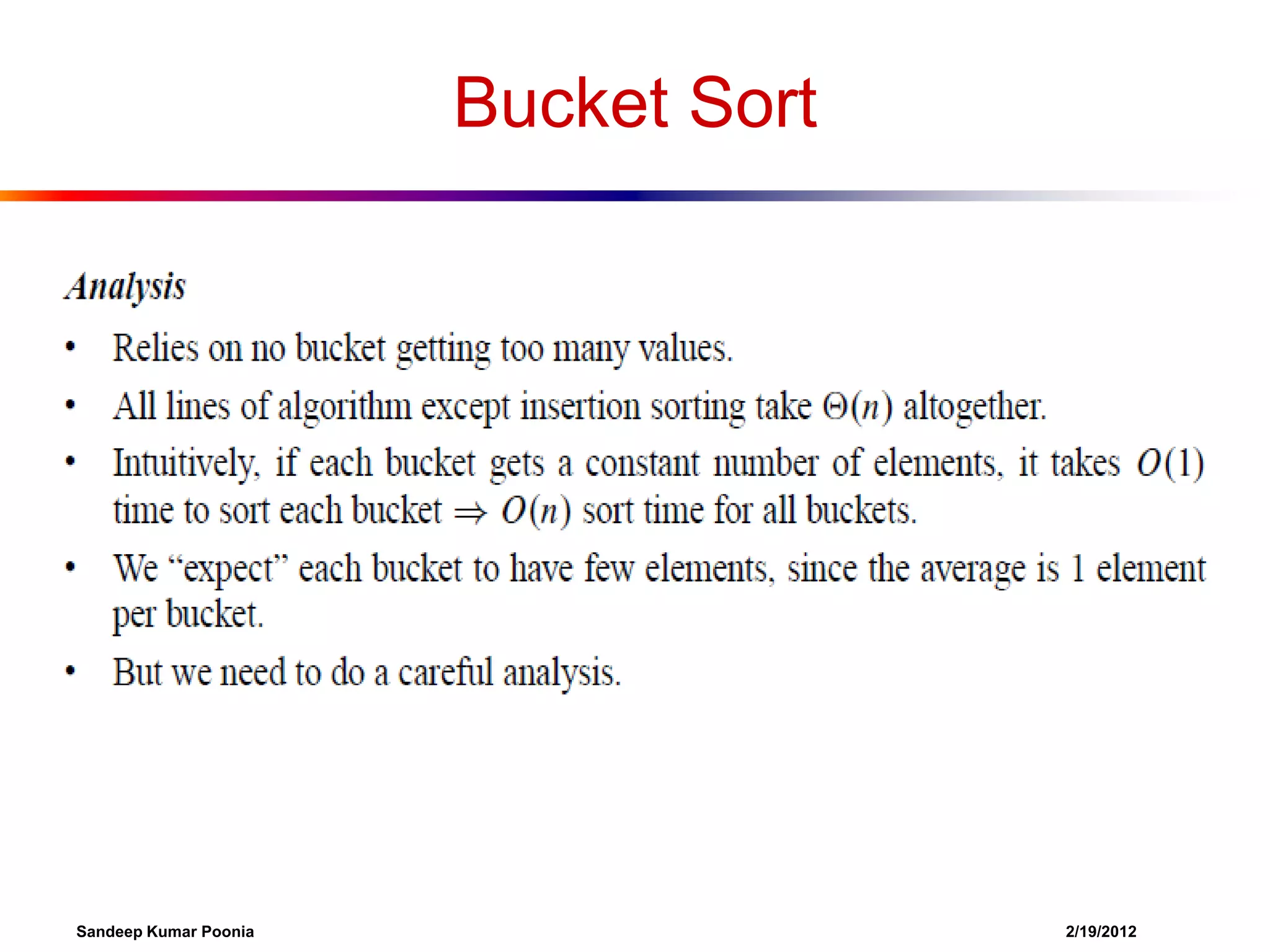

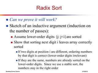
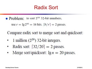
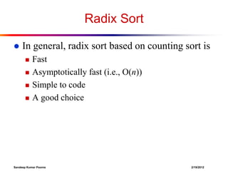
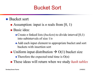
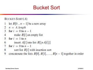
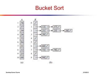
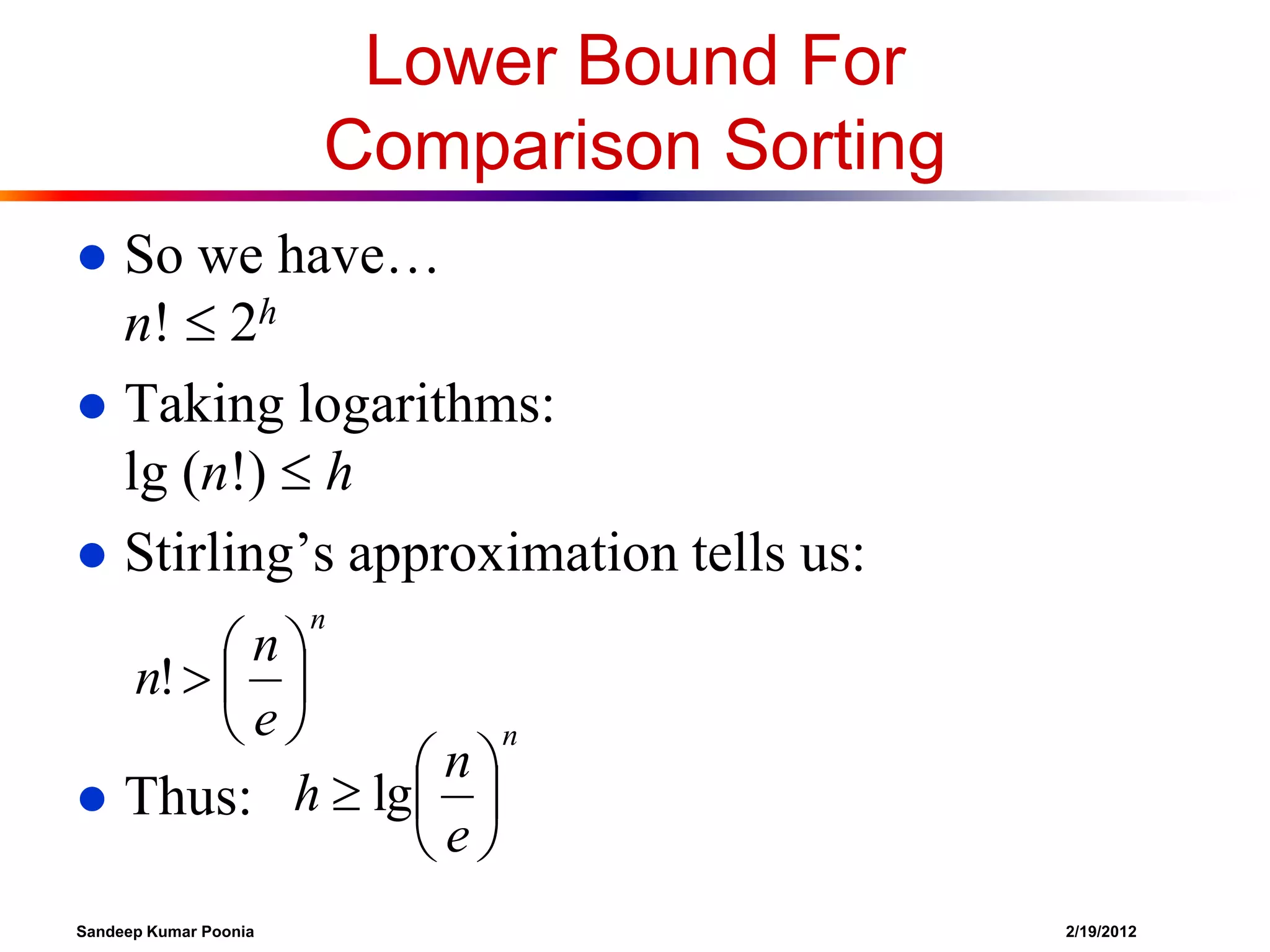
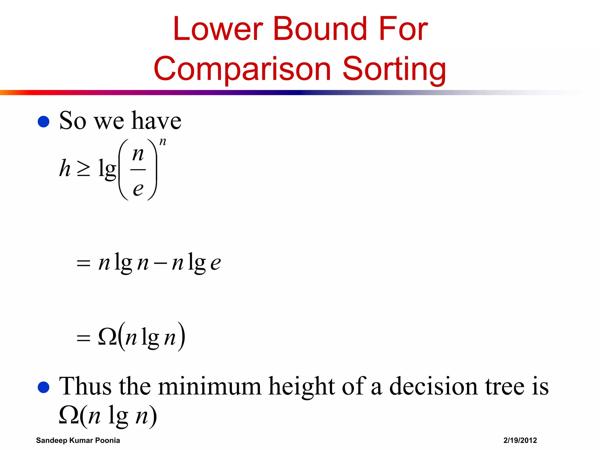
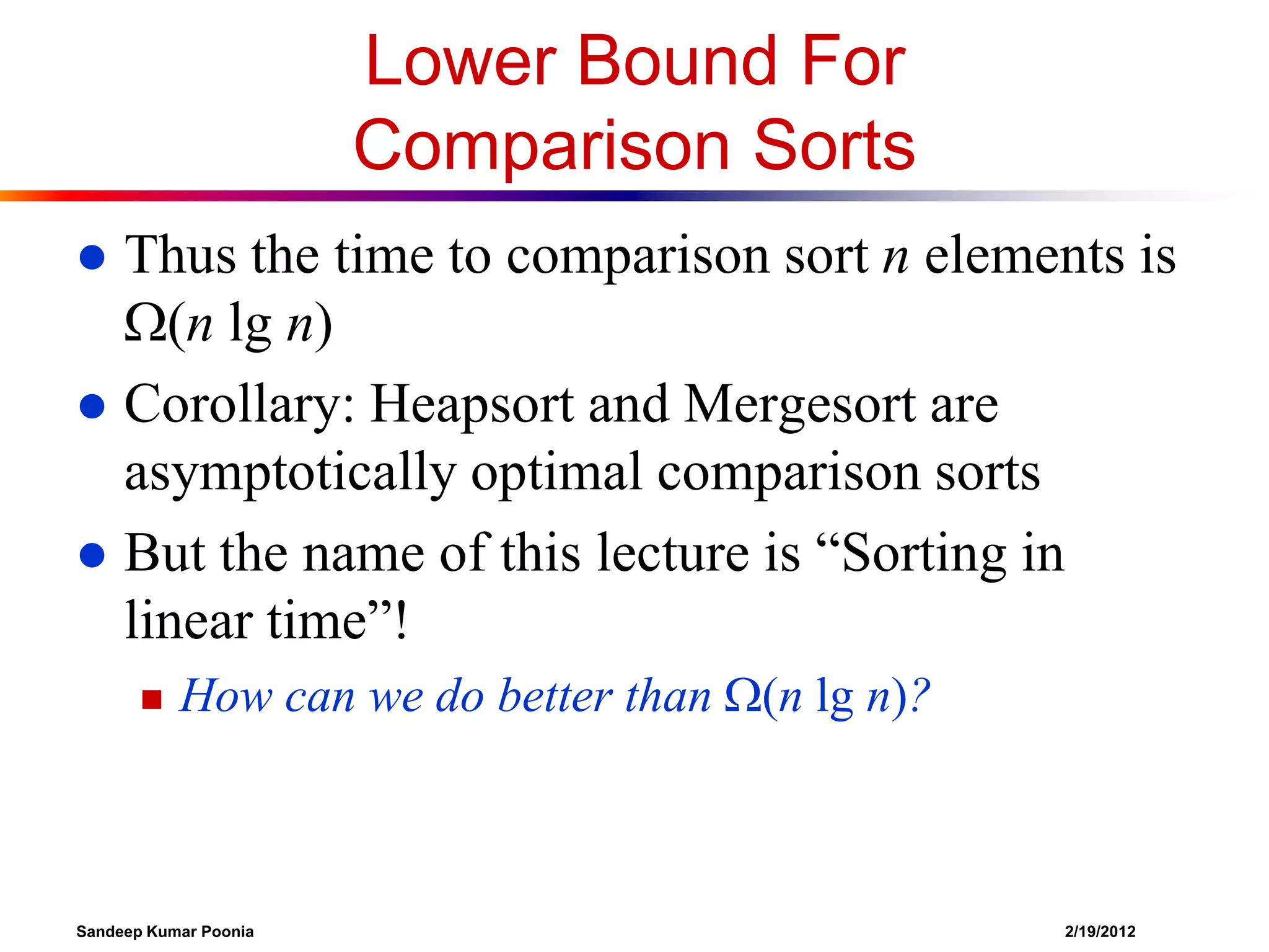
This document discusses various sorting algorithms and their time complexities, including linear-time sorting algorithms. It introduces counting sort, which can sort in O(n) time when the range of input values is small. Radix sort is then presented as a generalization of counting sort that can sort integers in linear time by sorting based on individual digit positions. Bucket sort is also discussed as another linear-time sorting algorithm when inputs are uniformly distributed.


