Downloaded 438 times


![MapReduce
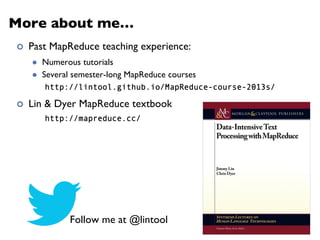
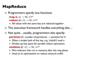
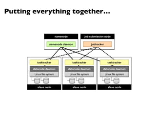
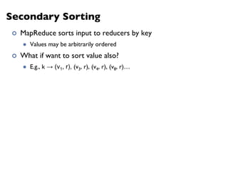
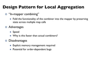
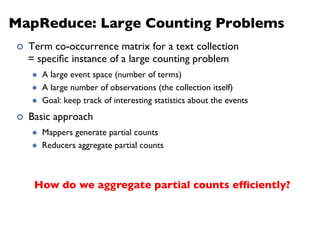
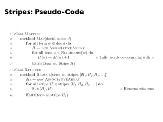
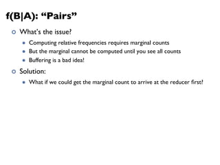
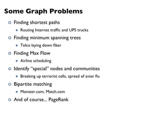
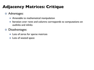
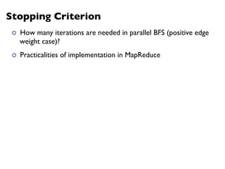
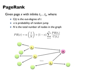
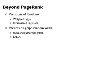
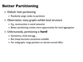
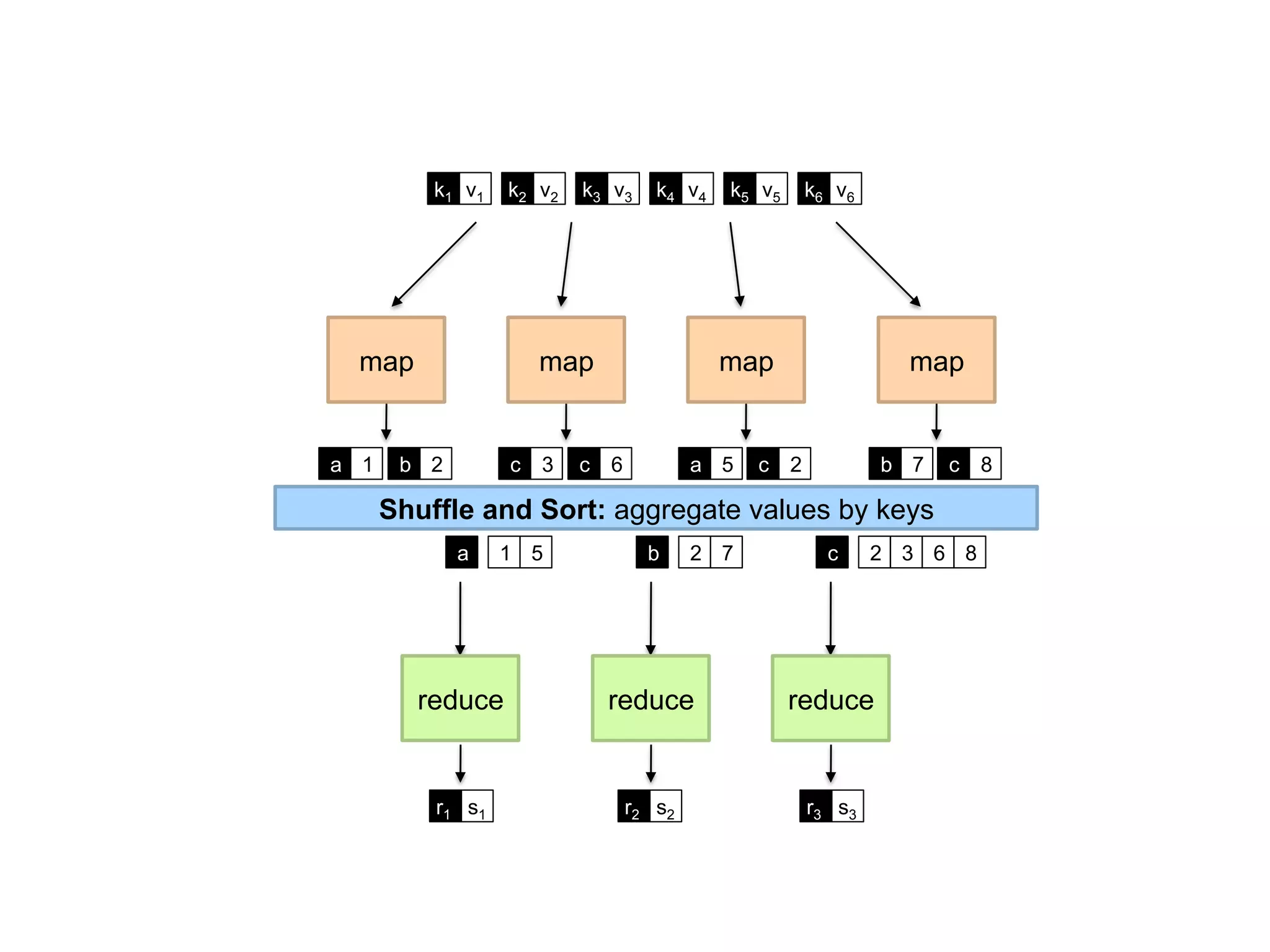
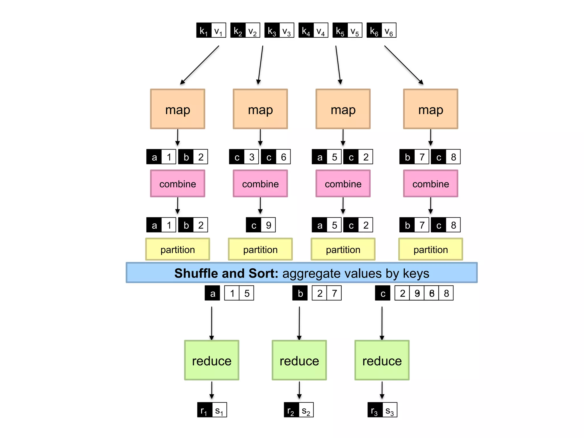
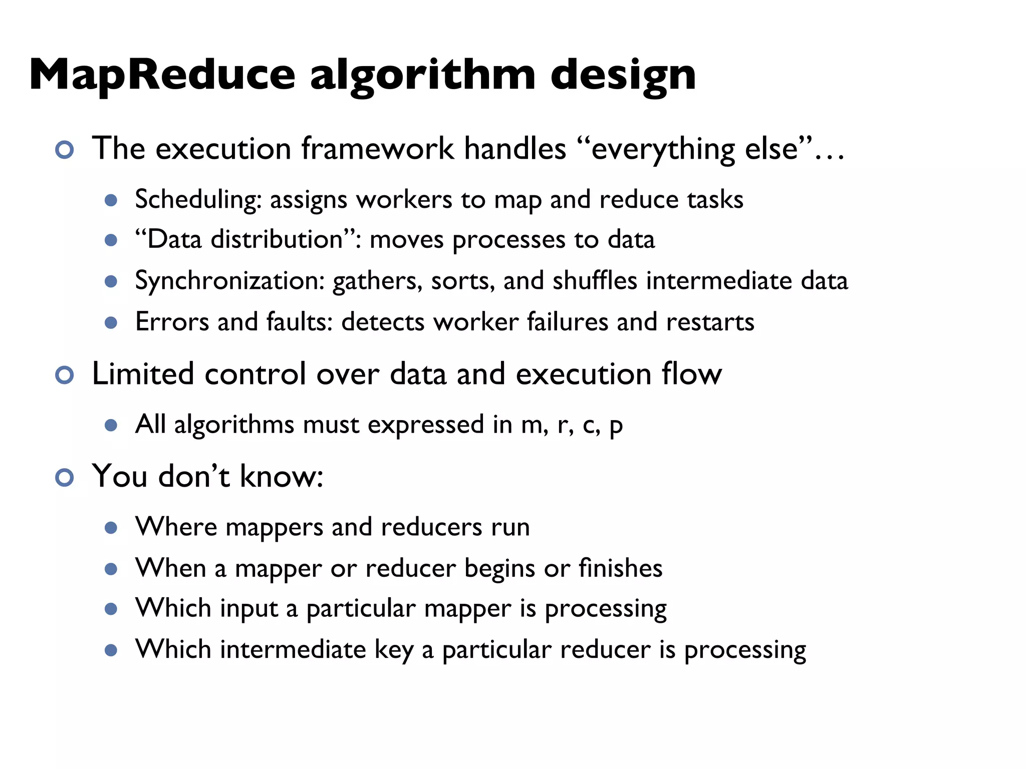
¢ Programmers specify two functions:
map (k1, v1) → [k2, v2]
reduce (k2, [v2]) → [k3, v3]
l All values with the same key are sent to the same reducer
¢ The execution framework handles everything else…](https://image.slidesharecdn.com/www2013-mapreduce-tutorial-slides-130513085031-phpapp02/85/MapReduce-Algorithm-Design-19-320.jpg)

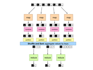


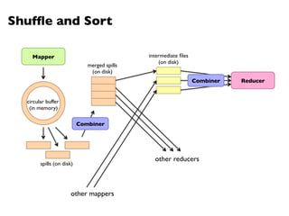
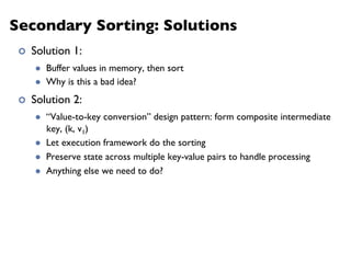


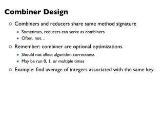


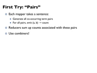

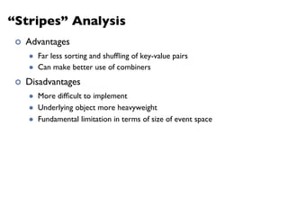


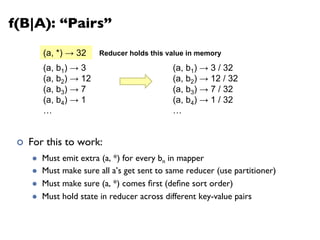

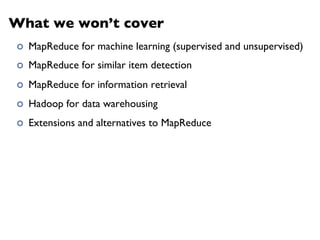
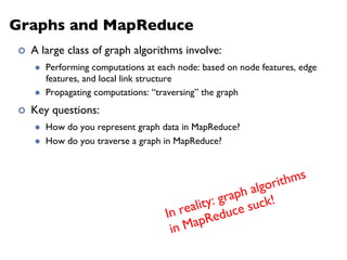
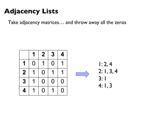
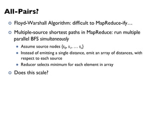
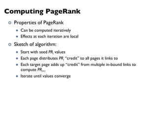
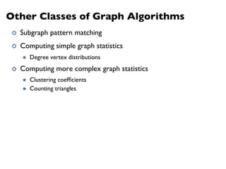
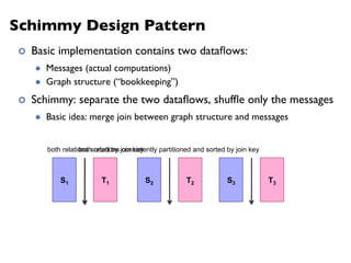
![Hidden Markov Models
An HMM is characterized by:
l N states:
l N x N Transition probability matrix
l V observation symbols:
l N x |V| Emission probability matrix
l Prior probabilities vector
aij = p(qj|qi)
X
j
aij = 1 8i
A = [aij]
NX
i=1
⇡i = 1
= (A, B, ⇧)
Q = {q1, q2, . . . qN }
O = {o1, o2, . . . oV }
B = [biv]
biv = bi(ov) = p(ov|qi)
⇧ = [⇡i, ⇡2, . . . ⇡N ]](https://image.slidesharecdn.com/www2013-mapreduce-tutorial-slides-130513085031-phpapp02/85/MapReduce-Algorithm-Design-71-320.jpg)
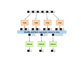
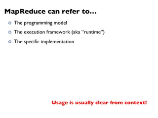
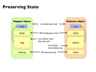
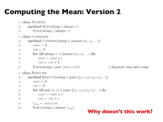
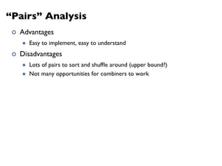
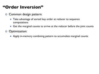
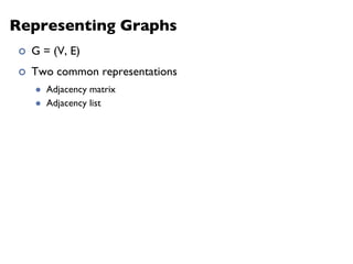
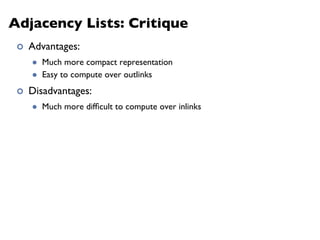
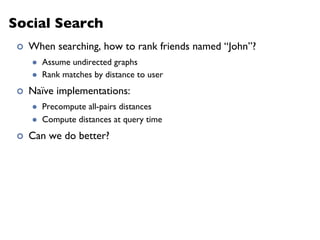
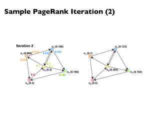
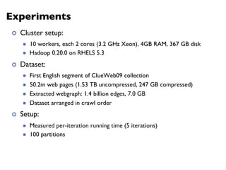
![MapReduce Implementation: Reducer
1: class Combiner
2: method Combine(string t, stripes [C1, C2, . . .])
3: Cf new AssociativeArray
4: for all stripe C 2 stripes [C1, C2, . . .] do
5: Sum(Cf , C)
6: Emit(string t, stripe Cf )
1: class Reducer
2: method Reduce(string t, stripes [C1, C2, . . .])
3: Cf new AssociativeArray
4: for all stripe C 2 stripes [C1, C2, . . .] do
5: Sum(Cf , C)
6: z 0
7: for all hk, vi 2 Cf do
8: z z + v
9: Pf new AssociativeArray . Final parameters vector
10: for all hk, vi 2 Cf do
11: Pf {k} v/z
12: Emit(string t, stripe Pf )
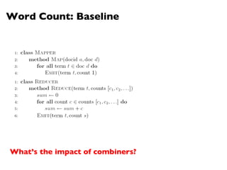
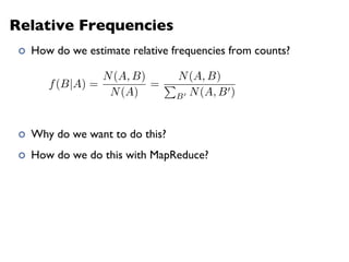
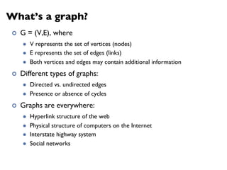
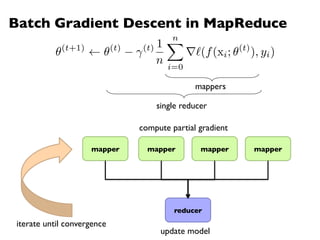
Figure 6.9: Combiner and reducer pseudo-code for training hidden Markov models using EM.
The HMMs considered in this book are fully parameterized by multinomial distributions, so
reducers do not require special logic to handle di↵erent types of model parameters (since they
are all of the same type).
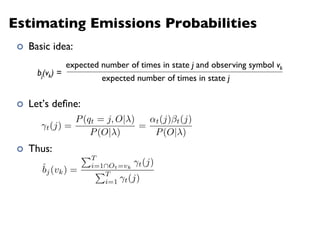
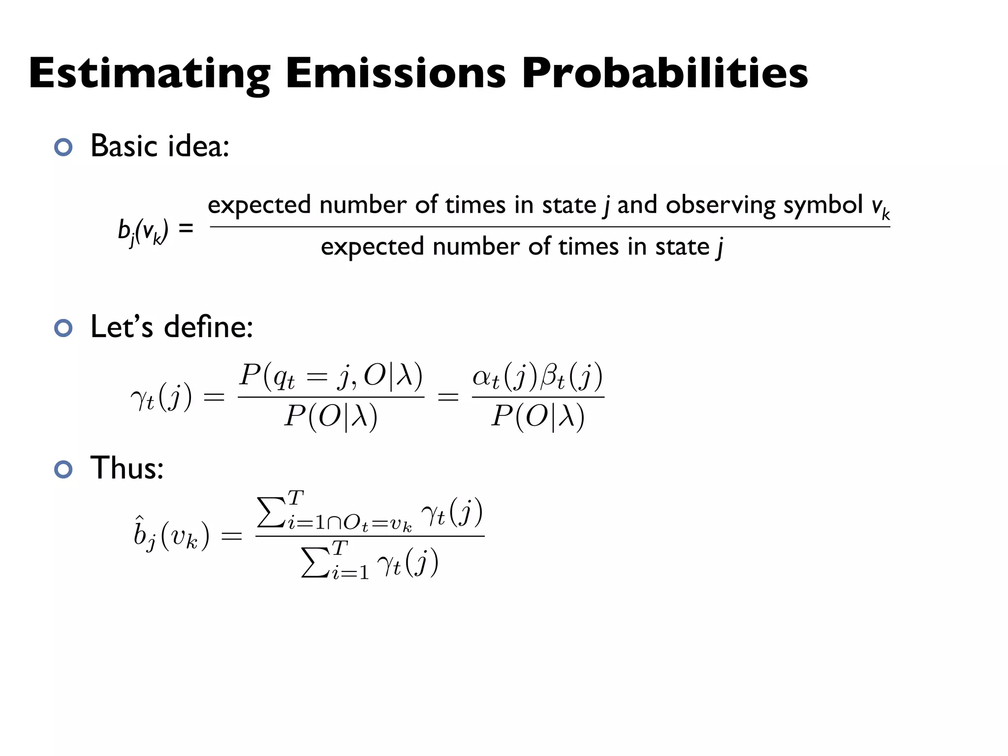
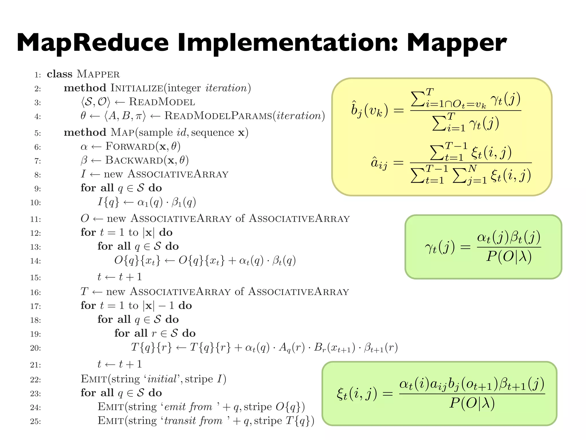
ˆbj(vk) =
PT
i=1Ot=vk
t(j)
PT
i=1 t(j)
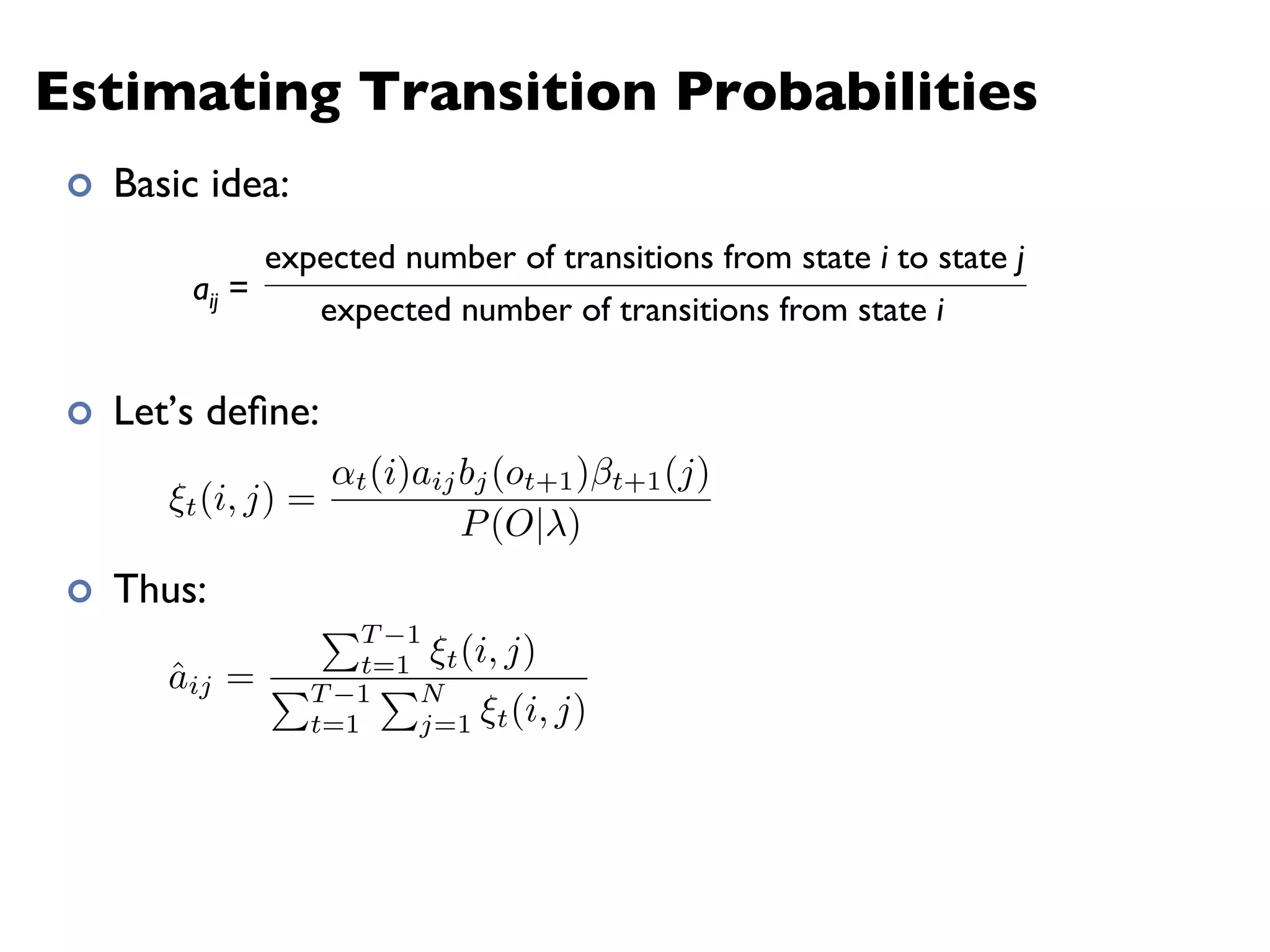
ˆaij =
PT 1
t=1 ⇠t(i, j)
PT 1
t=1
PN
j=1 ⇠t(i, j)
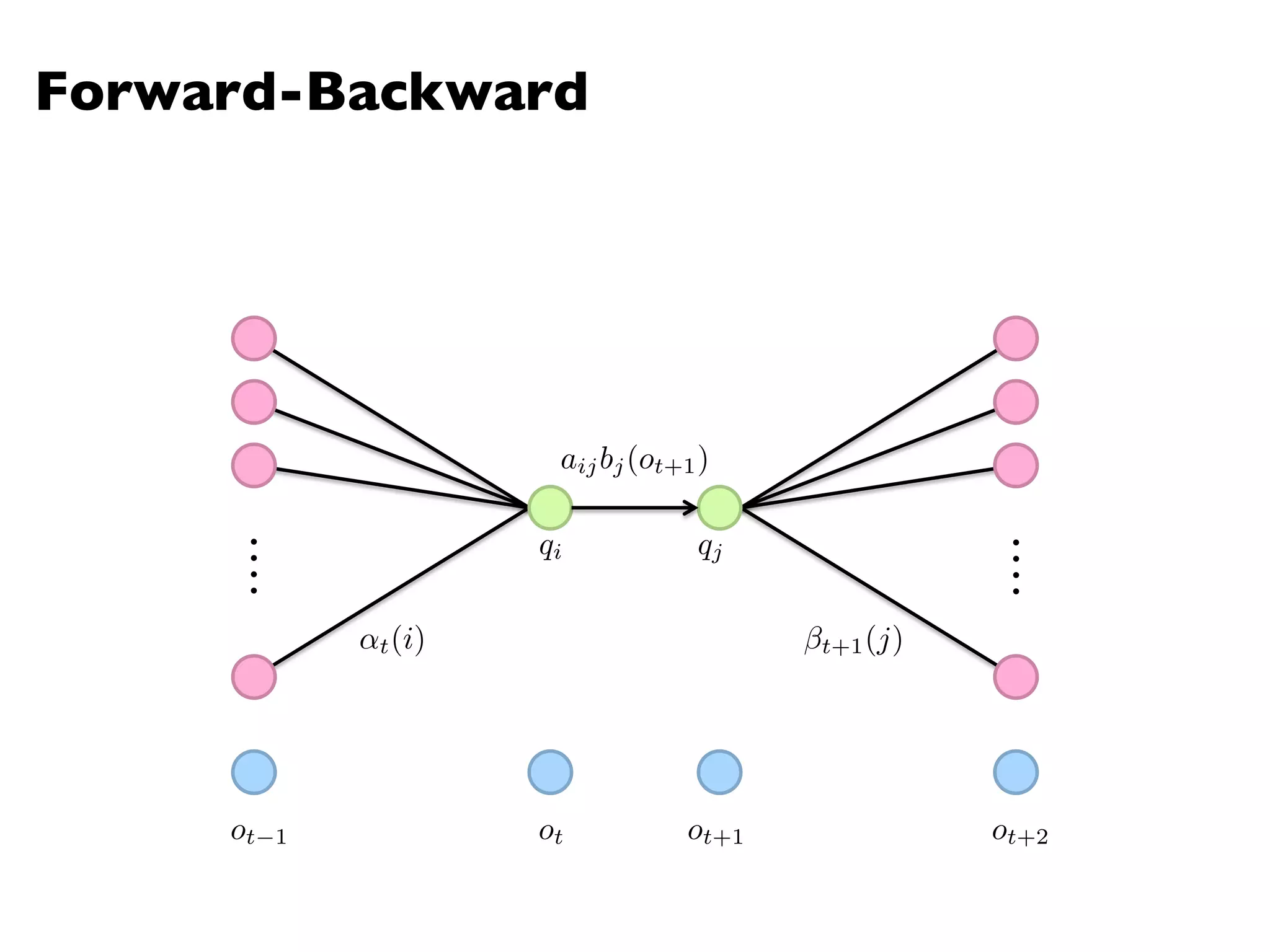
t(j) =
↵t(j) t(j)
P(O| )
⇠t(i, j) =
↵t(i)aijbj(ot+1) t+1(j)
P(O| )](https://image.slidesharecdn.com/www2013-mapreduce-tutorial-slides-130513085031-phpapp02/85/MapReduce-Algorithm-Design-77-320.jpg)


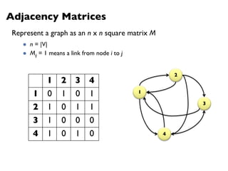
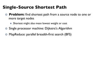


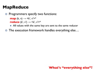
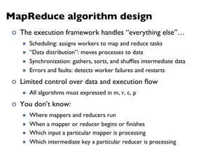
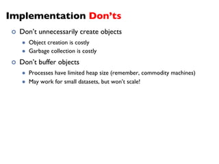
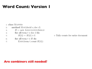
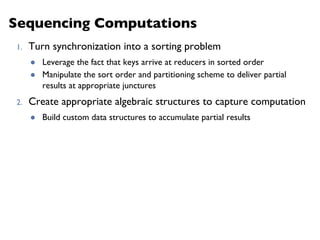
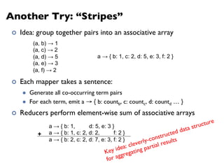
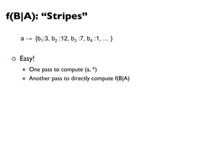
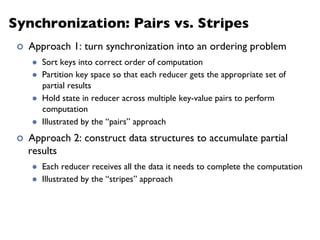
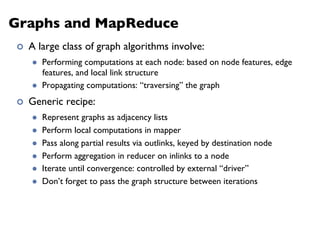
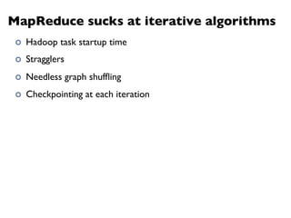
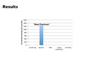
![Landmark Approach (aka sketches)
¢ Select n seeds {s0, s1, … sn}
¢ Compute distances from seeds to every node:
l What can we conclude about distances?
l Insight: landmarks bound the maximum path length
¢ Lots of details:
l How to more tightly bound distances
l How to select landmarks (random isn’t the best…)
¢ Use multi-source parallel BFS implementation in MapReduce!
A
=
[2, 1, 1]
B
=
[1, 1, 2]
C
=
[4, 3, 1]
D
=
[1, 2, 4]](https://image.slidesharecdn.com/www2013-mapreduce-tutorial-slides-130513085031-phpapp02/85/MapReduce-Algorithm-Design-105-320.jpg)


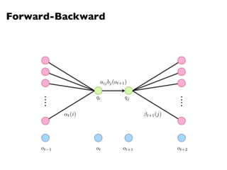
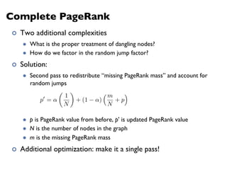
![PageRank in MapReduce
n5 [n1, n2, n3]n1 [n2, n4] n2 [n3, n5] n3 [n4] n4 [n5]
n2 n4 n3 n5 n1 n2 n3n4 n5
n2 n4n3 n5n1 n2 n3 n4 n5
n5 [n1, n2, n3]n1 [n2, n4] n2 [n3, n5] n3 [n4] n4 [n5]
Map
Reduce](https://image.slidesharecdn.com/www2013-mapreduce-tutorial-slides-130513085031-phpapp02/85/MapReduce-Algorithm-Design-113-320.jpg)


![MapReduce
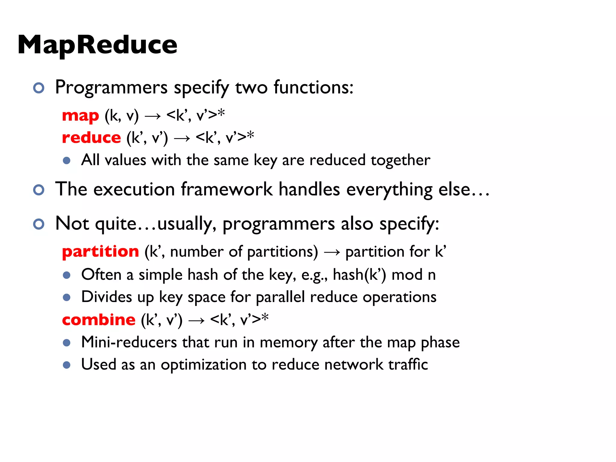
¢ Programmers specify two functions:
map (k1, v1) → [k2, v2]
reduce (k2, [v2]) → [k3, v3]
l All values with the same key are sent to the same reducer
¢ The execution framework handles everything else…](https://image.slidesharecdn.com/www2013-mapreduce-tutorial-slides-130513085031-phpapp02/75/MapReduce-Algorithm-Design-19-2048.jpg)


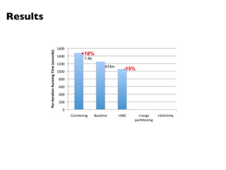
![Hidden Markov Models
An HMM is characterized by:
l N states:
l N x N Transition probability matrix
l V observation symbols:
l N x |V| Emission probability matrix
l Prior probabilities vector
aij = p(qj|qi)
X
j
aij = 1 8i
A = [aij]
NX
i=1
⇡i = 1
= (A, B, ⇧)
Q = {q1, q2, . . . qN }
O = {o1, o2, . . . oV }
B = [biv]
biv = bi(ov) = p(ov|qi)
⇧ = [⇡i, ⇡2, . . . ⇡N ]](https://image.slidesharecdn.com/www2013-mapreduce-tutorial-slides-130513085031-phpapp02/75/MapReduce-Algorithm-Design-71-2048.jpg)
![MapReduce Implementation: Reducer
1: class Combiner
2: method Combine(string t, stripes [C1, C2, . . .])
3: Cf new AssociativeArray
4: for all stripe C 2 stripes [C1, C2, . . .] do
5: Sum(Cf , C)
6: Emit(string t, stripe Cf )
1: class Reducer
2: method Reduce(string t, stripes [C1, C2, . . .])
3: Cf new AssociativeArray
4: for all stripe C 2 stripes [C1, C2, . . .] do
5: Sum(Cf , C)
6: z 0
7: for all hk, vi 2 Cf do
8: z z + v
9: Pf new AssociativeArray . Final parameters vector
10: for all hk, vi 2 Cf do
11: Pf {k} v/z
12: Emit(string t, stripe Pf )
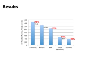
Figure 6.9: Combiner and reducer pseudo-code for training hidden Markov models using EM.
The HMMs considered in this book are fully parameterized by multinomial distributions, so
reducers do not require special logic to handle di↵erent types of model parameters (since they
are all of the same type).
ˆbj(vk) =
PT
i=1Ot=vk
t(j)
PT
i=1 t(j)
ˆaij =
PT 1
t=1 ⇠t(i, j)
PT 1
t=1
PN
j=1 ⇠t(i, j)
t(j) =
↵t(j) t(j)
P(O| )
⇠t(i, j) =
↵t(i)aijbj(ot+1) t+1(j)
P(O| )](https://image.slidesharecdn.com/www2013-mapreduce-tutorial-slides-130513085031-phpapp02/75/MapReduce-Algorithm-Design-77-2048.jpg)


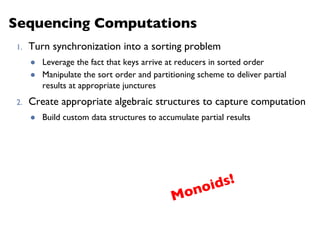
![Landmark Approach (aka sketches)
¢ Select n seeds {s0, s1, … sn}
¢ Compute distances from seeds to every node:
l What can we conclude about distances?
l Insight: landmarks bound the maximum path length
¢ Lots of details:
l How to more tightly bound distances
l How to select landmarks (random isn’t the best…)
¢ Use multi-source parallel BFS implementation in MapReduce!
A
=
[2, 1, 1]
B
=
[1, 1, 2]
C
=
[4, 3, 1]
D
=
[1, 2, 4]](https://image.slidesharecdn.com/www2013-mapreduce-tutorial-slides-130513085031-phpapp02/75/MapReduce-Algorithm-Design-105-2048.jpg)

![PageRank in MapReduce
n5 [n1, n2, n3]n1 [n2, n4] n2 [n3, n5] n3 [n4] n4 [n5]
n2 n4 n3 n5 n1 n2 n3n4 n5
n2 n4n3 n5n1 n2 n3 n4 n5
n5 [n1, n2, n3]n1 [n2, n4] n2 [n3, n5] n3 [n4] n4 [n5]
Map
Reduce](https://image.slidesharecdn.com/www2013-mapreduce-tutorial-slides-130513085031-phpapp02/75/MapReduce-Algorithm-Design-113-2048.jpg)


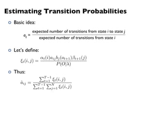
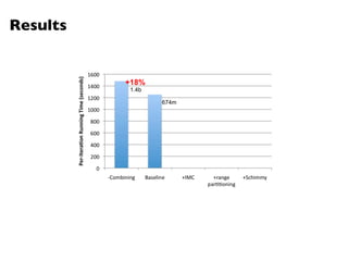
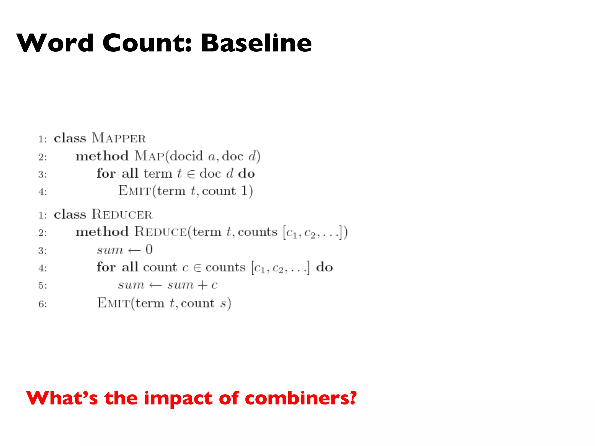
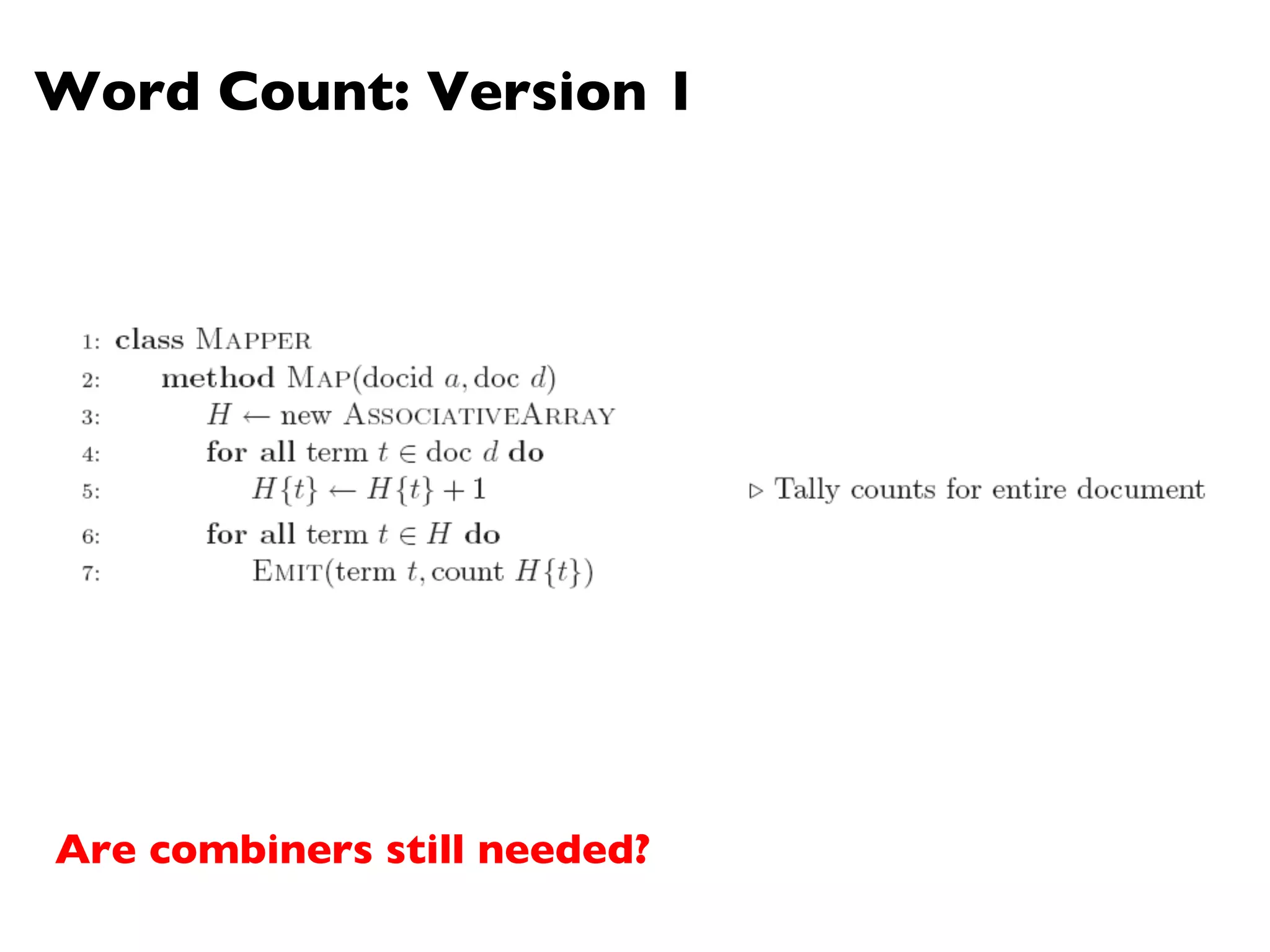
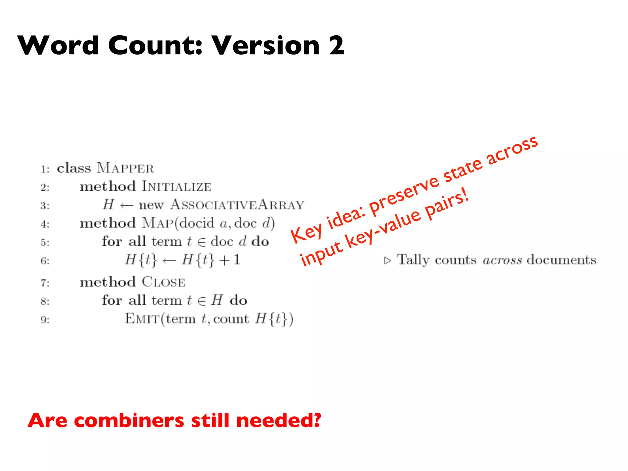
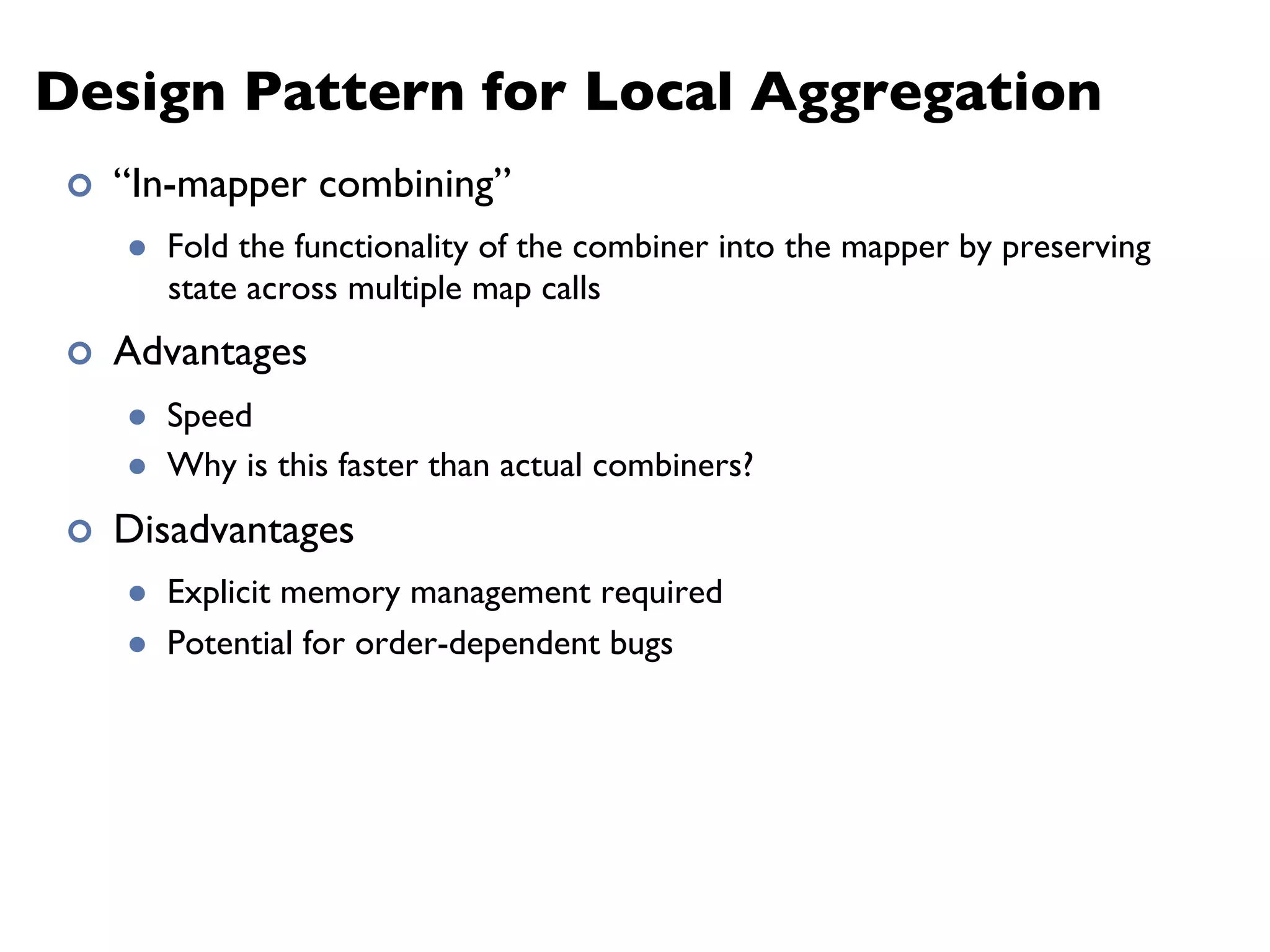
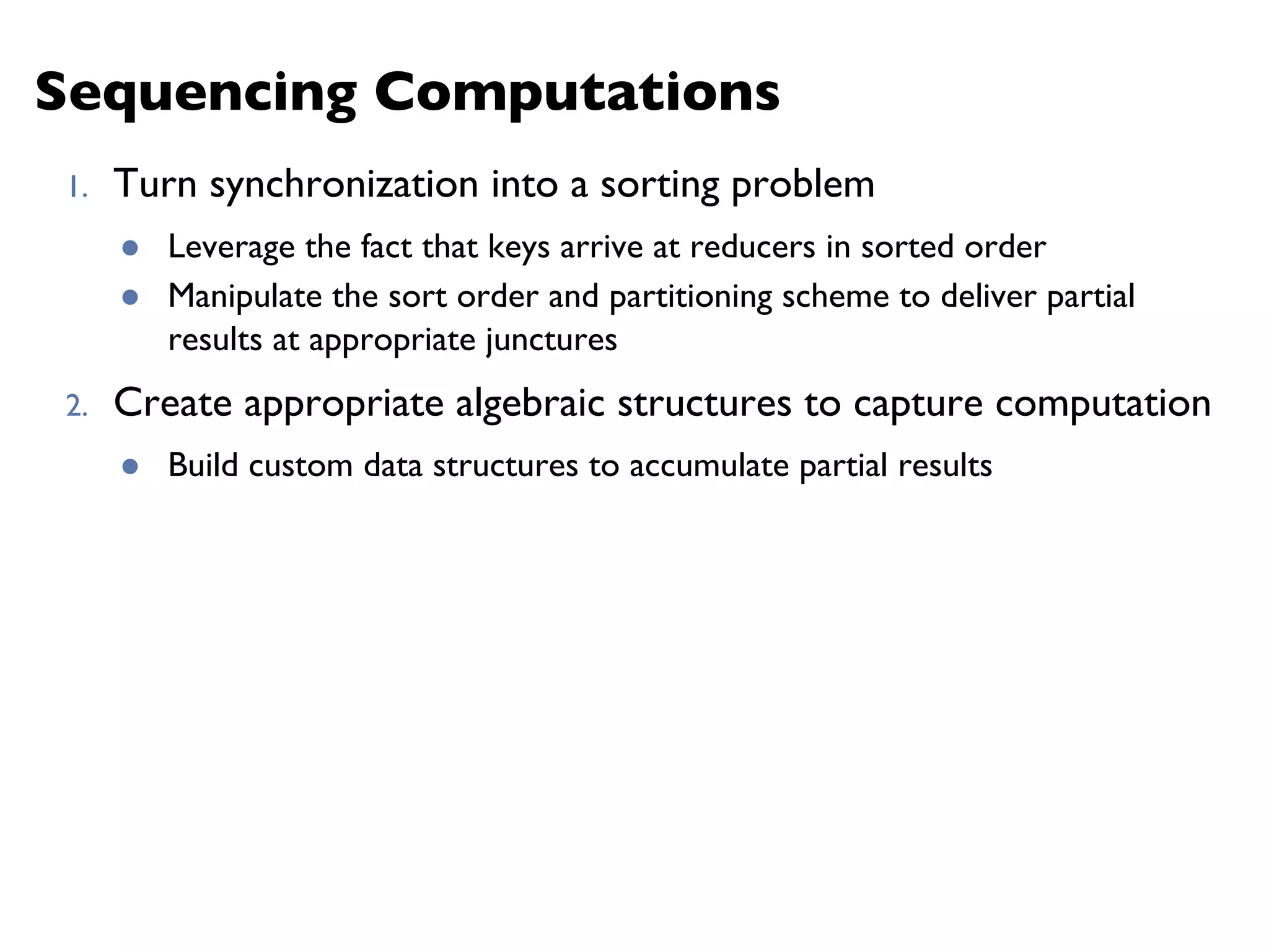
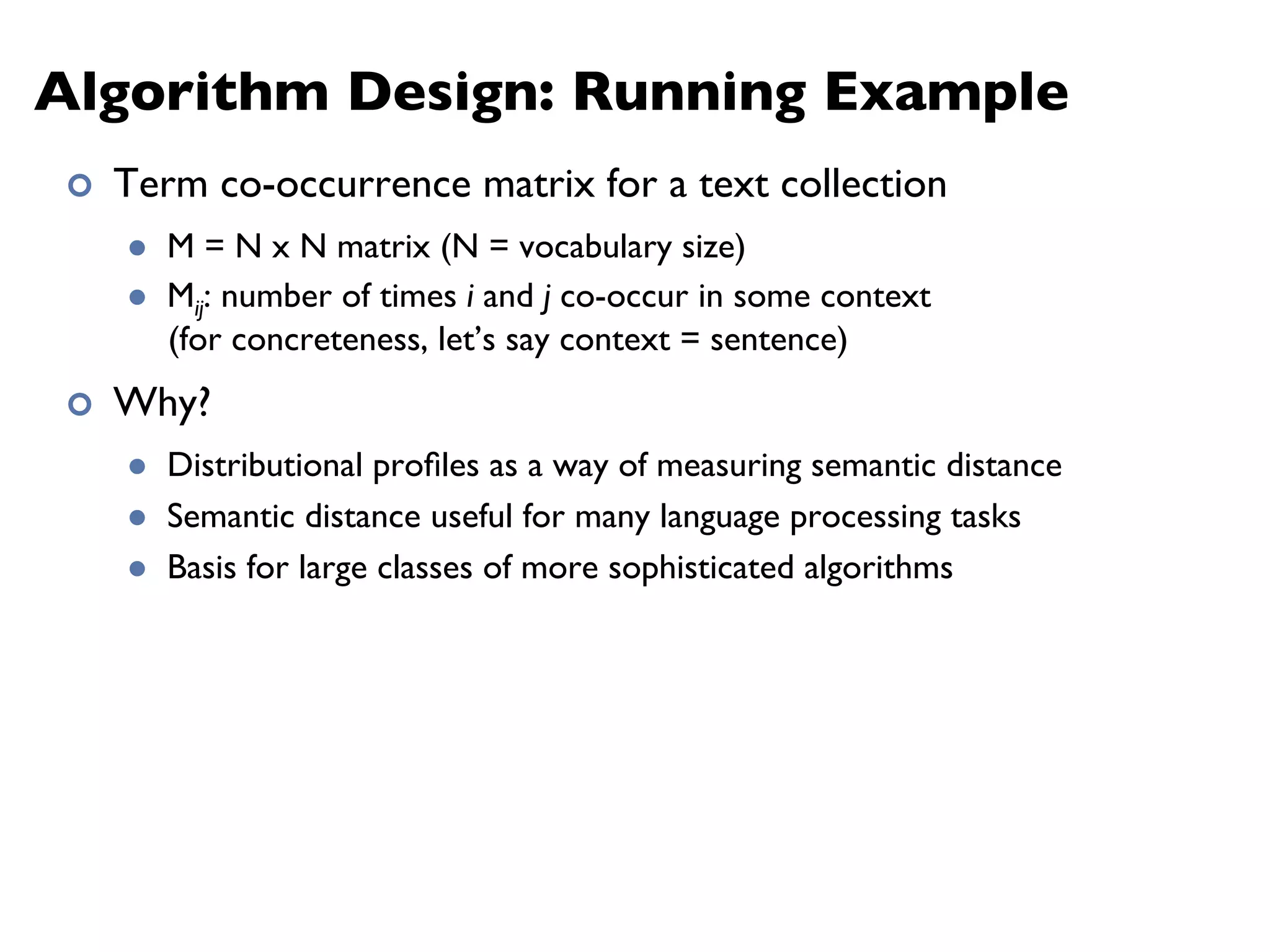
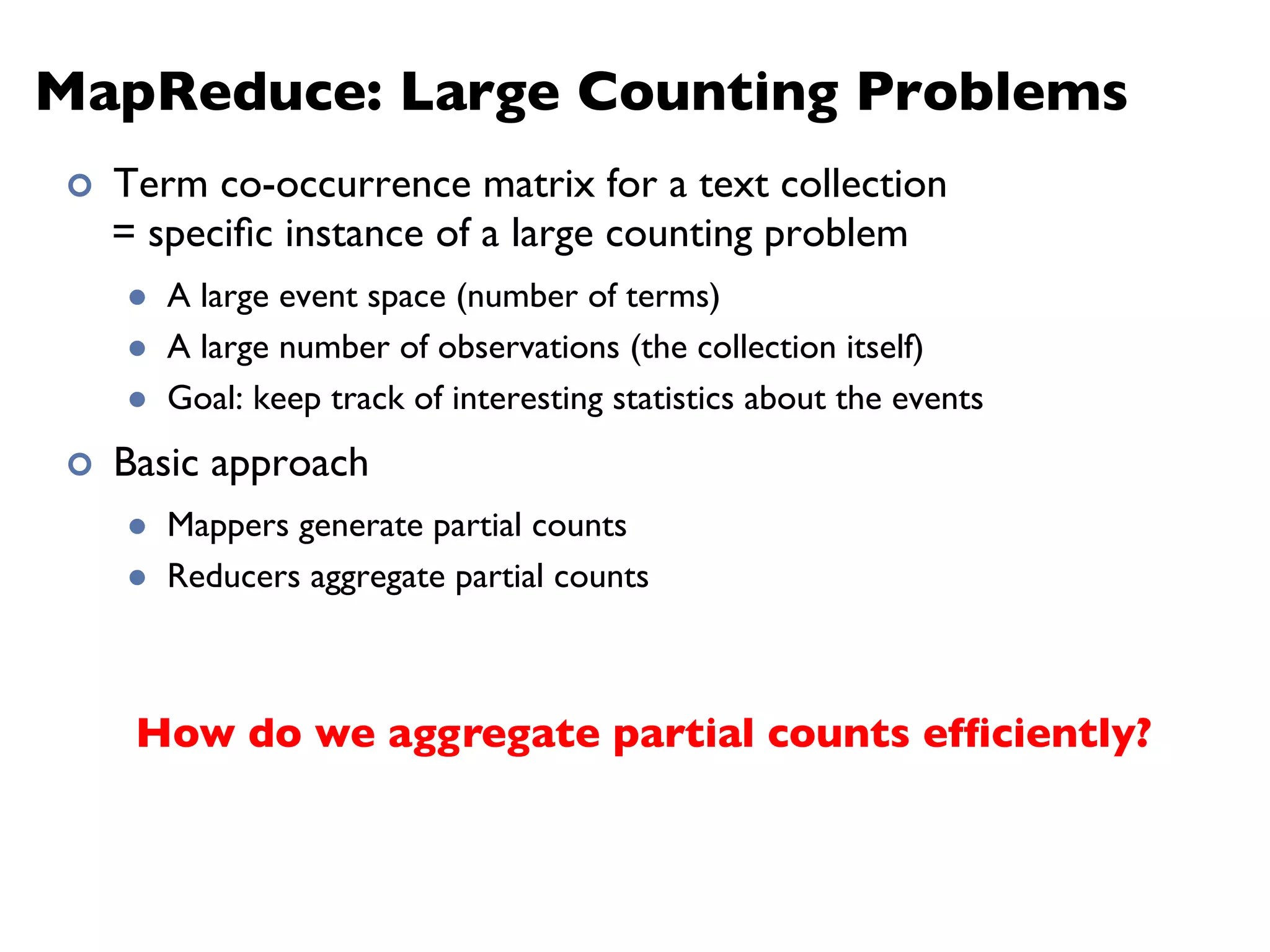
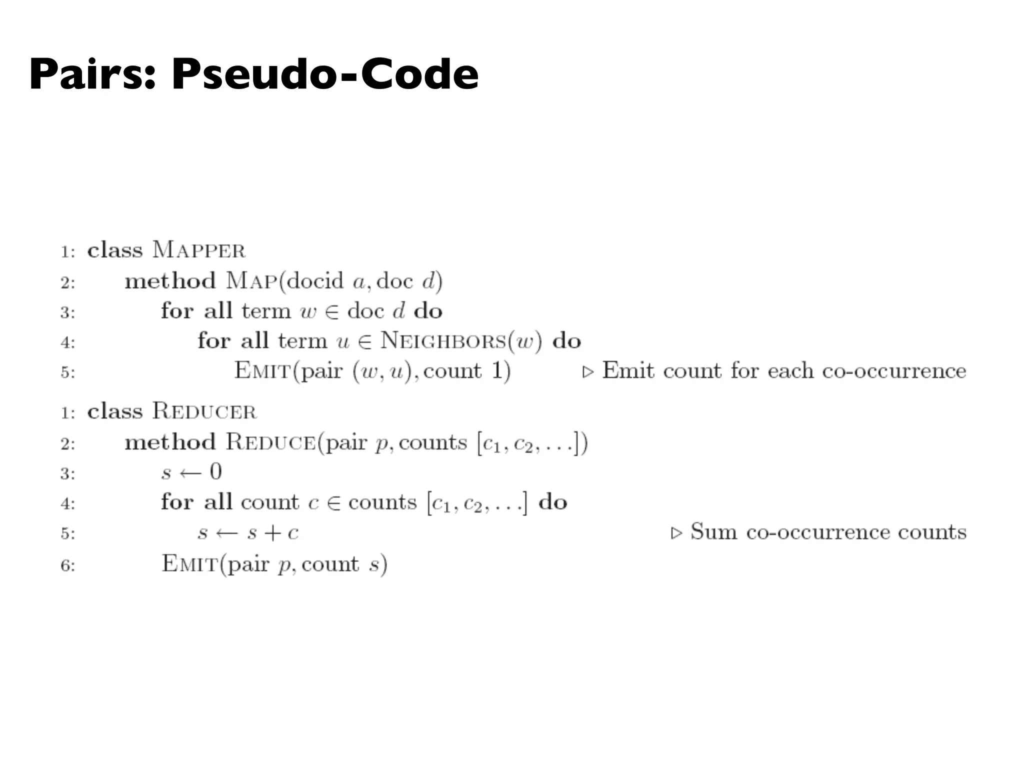
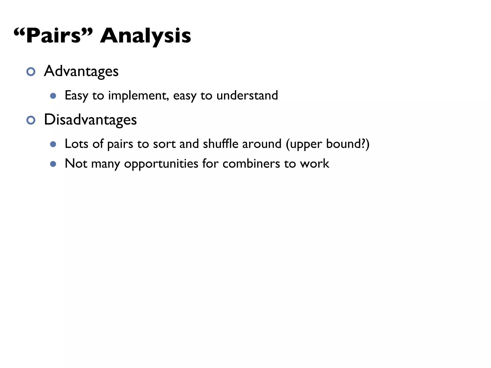
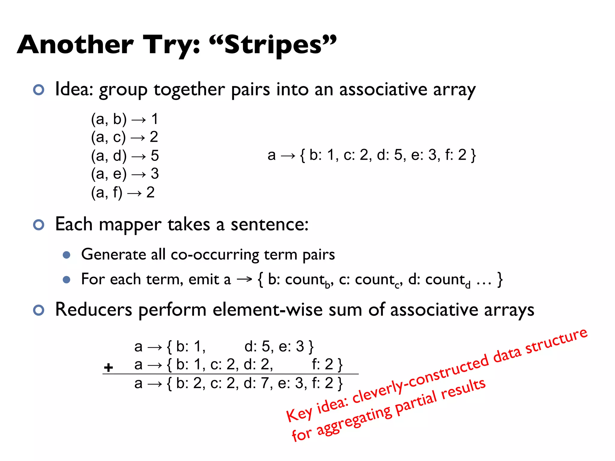
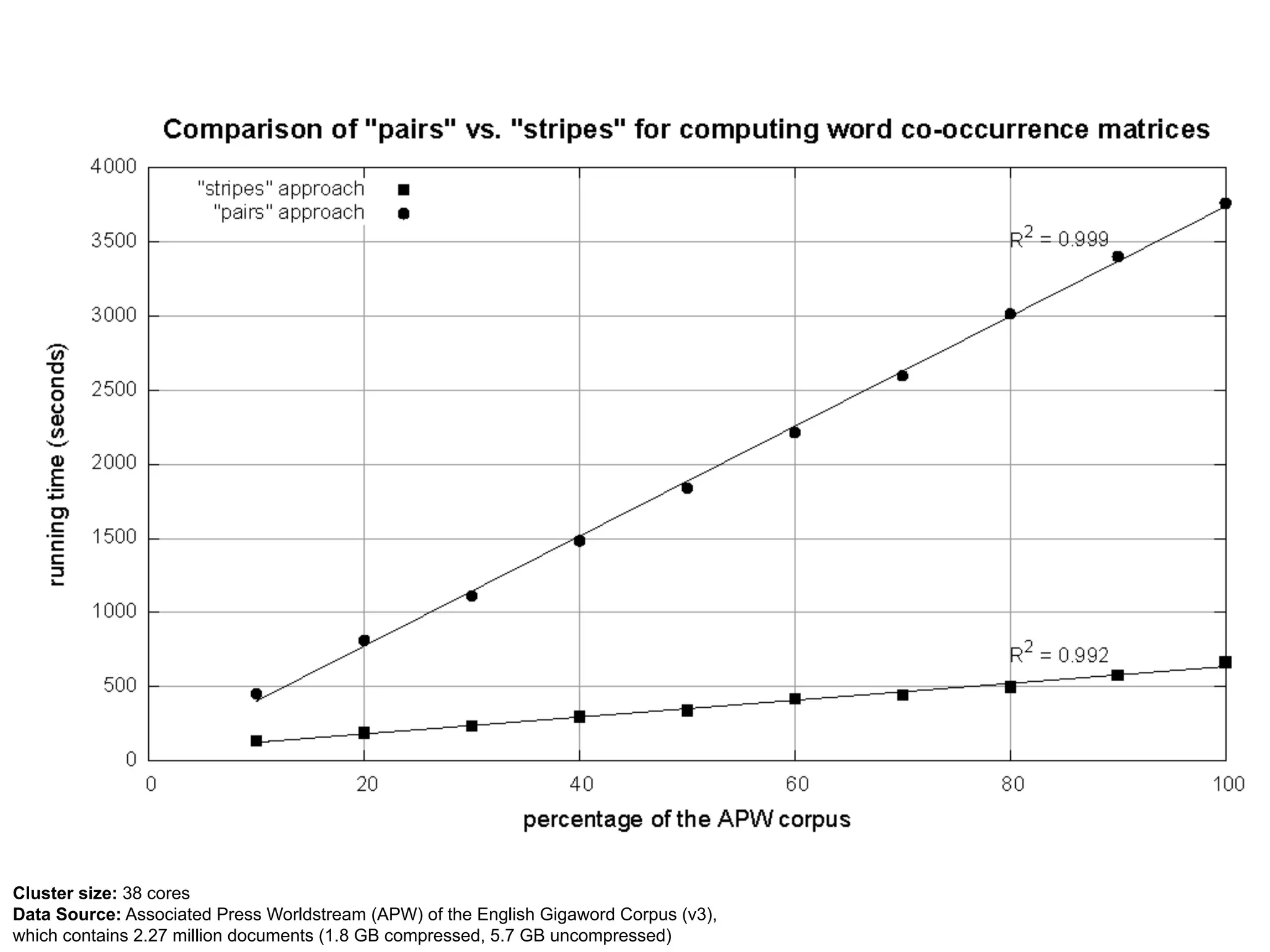
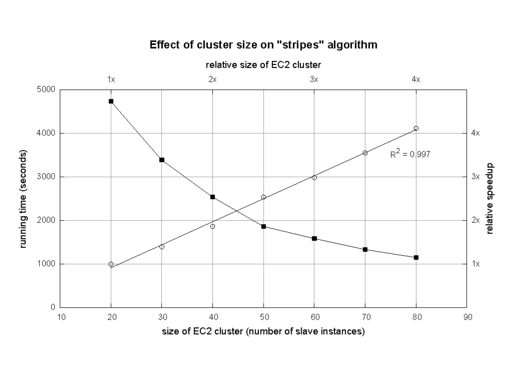
The document summarizes Jimmy Lin's MapReduce tutorial for WWW 2013. It discusses the MapReduce algorithm design and implementation. Specifically, it covers key aspects of MapReduce like local aggregation to reduce network traffic, sequencing computations by manipulating sort order, and using appropriate data structures to accumulate results incrementally. It also provides an example of building a term co-occurrence matrix to measure semantic distance between words.


