This document is Brian Flynn's final year thesis at Trinity College Dublin titled "Mathematical Introduction to Quantum Computation". It provides an introduction to the fundamental concepts of quantum computing through a mathematical lens. The thesis aims to explain quantum computing in a clear and accessible way. It begins by reviewing some linear algebra concepts needed to describe quantum mechanics. It then discusses the postulates of quantum mechanics and introduces the idea of quantum superpositions. The document outlines how these quantum principles can be used to define quantum bits and develop the basic building blocks of quantum gates and circuits. It explores some computational techniques and algorithms uniquely possible with quantum computers, like Shor's factoring algorithm. The overall goal of the thesis is to convey the key mathematical


![1.1. MOTIVATION CHAPTER 1. introduction
1.1 motivation
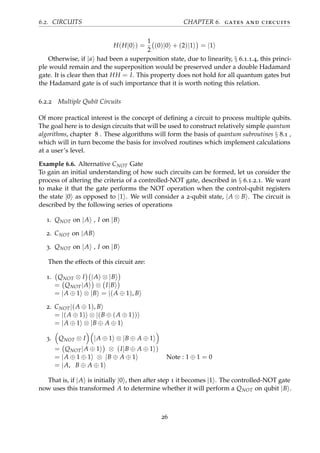
Since the notion of a quantum computer was first suggested by Yuri Manin in 1980 [1],
and seperately by Richard Feynman [2], many prominent mathematicians and physicists
have studied the topic in great depth. In 1982, the first potential framework of a quantum
computer was proposed by Paul Benioff [3]. In the following years, it was proven that
there were processes for which quantum computing could be shown to out-perform its
classical counterpart, in particular by the work of David Deutsch, [4]. In 1992, Deutsch,
together with Richard Josza released a paper entitled Rapid solution of problems by quan-
tum computation, in which they showed how quantum machines could be used to achieve
exponential speed-up in solving computational problems [5]. The problems that their al-
gorithm was able to solve, however, were of little practical use, so there was no known
reason to actually invest in the construction of such potentially useless devices. In 1994,
Peter Shor published a paper that became a turning point in the history of quantum
computing: his now-famous algorithm used techniques only available to quantum com-
puters to solve factorisation problems. He showed that a quantum computer would be
able to factorise large numbers with significantly less computational expense than clas-
sical machines will ever be capable of [6]. Following this milestone, it became clear that
quantum methods have the capacity to transcend classical machines, and so the field has
been growing steadily as a research topic since.
In the late 1990’s, the first quantum computer was built utilising 2 qubits. There have
been significant strides every year since then towards a fully functional model.
Thus our motivation is clear: the entire quantum computing industry is built on the
belief that, quite soon, we will be able to build computers which operate at exponen-
tially faster and more efficient rates than we will ever be able to achieve using classical
implementations.
We endeavour to understand the building blocks which are at the centre of this po-
tentially massive transition to a new kind of computation.
3](https://image.slidesharecdn.com/b93d7c4e-484e-4e7c-9a0b-90813b0817a5-160722100840/85/Mathematical_Introduction_to_Quantum_Computation-8-320.jpg)
![2
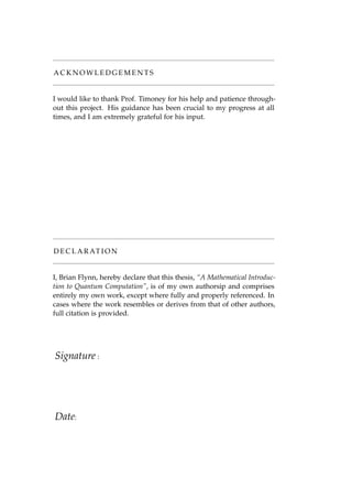
L I N E A R A L G E B R A
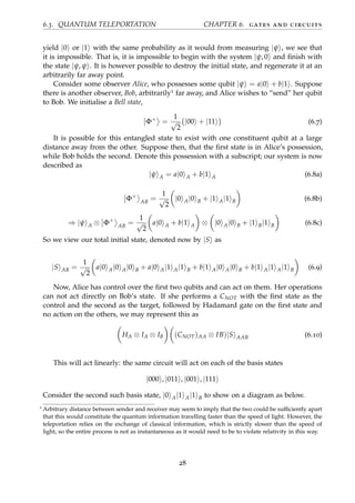
Before getting too involved in mechanical view points and quantum physics, it is im-
portant to review the language with which these topics will be discussed: here we will
recap some basics of linear algebra and summarise the basic mathematical techniques
required to describe physics at a quantum scale.
2.1 recap of basics
Some algebraic knowledge is assumed of the reader. For further discussion and deriva-
tion of some points, consult §2.1 of the standard text on the subject on quantum comput-
ing and information processing, Nielsen and Chuang. [7]. We will briefly recall some
definitions for reference.
• Notation
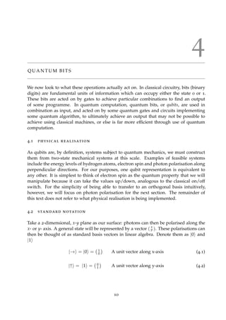
Definition of Representation
Vector (or ket) |ψ
Dual Vector (or bra) ψ|
Tensor Product |ψ ⊗ |φ
Complex conjugate |ψ∗
Transpose |ψ T
Adjoint |ψ †
= (|ψ ∗
)T
Algebraic Definitions
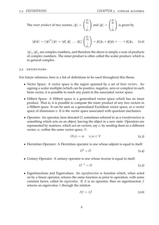
The dual vector of a vector (ket) |ψ is given by ψ| = |ψ †
. The adjoint of a matrix
replaces each matrix element with its own complex conjugate, and then switches
its columns with rows.
M†
=
M0,0 M0,1
M1,0 M1,1
†
=
M∗
0,0 M∗
0,1
M∗
1,0 M∗
1,1
T
=
M∗
0,0 M∗
1,0
M∗
0,1 M∗
1,1
(2.1)
5](https://image.slidesharecdn.com/b93d7c4e-484e-4e7c-9a0b-90813b0817a5-160722100840/85/Mathematical_Introduction_to_Quantum_Computation-10-320.jpg)

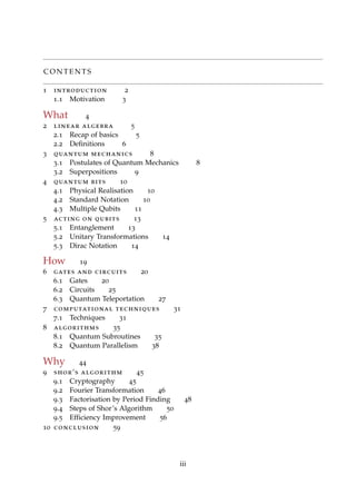
![4.3. MULTIPLE QUBITS CHAPTER 4. quantum bits
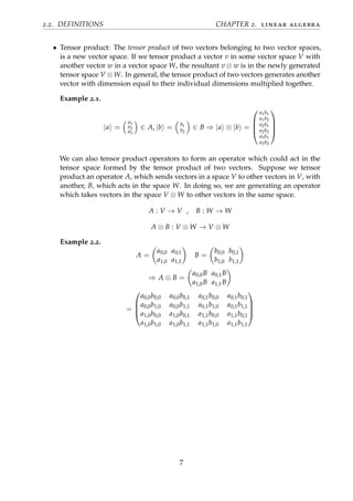
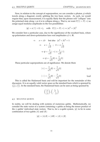
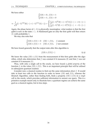
Consider first a simple system of 2 qubits. Measuring in the standard basis, these
qubits will have to collapse in to one of the basis states |0, 0 , |0, 1 , |1, 0 , |1, 1 . Thus, for
such a 2-qubit system, we have the general superposition
|ψ = α0,0|0, 0 + α0,1|0, 1 + α1,0|1, 0 + α1,1|1, 1
where αi,j is the amplitude for measuring the system as the state |i, j . This is perfectly
analogous to a classical 2-bit system necessarily occupying one of the four possibilities
(0, 0), (0, 1), (1, 0), (1, 1).
Hence, for example, if we wanted to concoct a two-qubit system composed of one
qubit in the state |+ and one in |−
|ψ = |+ ⊗ |−
|ψ = (
1
√
2
|0 +
1
√
2
|1 ) ⊗ (
1
√
2
|0 −
1
√
2
|1 )
=
1
2
[|00 − |01 + |10 − |11 ]
=
1
2
1
0 ⊗ 1
0 − 1
0 ⊗ 0
1 + 0
1 ⊗ 1
0 − 0
1 ⊗ 0
1
=
1
2
1
0
0
0
−
0
1
0
0
+
0
0
1
0
−
0
0
0
1
|ψ =
1
2
1
−1
−1
1
That is, the system is given by a linear combination of the four basis vectors
1
0
0
0
,
0
1
0
0
,
0
0
1
0
,
0
0
0
1
We can notice that a single qubit system can be described by a linear combination of two
basis vectors, and that a two qubit system requires four basis vectors to describe it. In
general we can say that an n-qubit system is represented by a linear combination of 2n
basis vectors.
4.3.1 Registers
A register is the name given to a system of multiple qubits. We may use the idea to
consider a system of n qubits as two sub systems. For instance, a register of ten qubits
can be denoted |x[10] , and we can think of the system as a register of six qubits together
with a register of three and another register of one qubit.
|x[10] = |x1[6] ⊗ |x2[3] ⊗ |x3[1]
12](https://image.slidesharecdn.com/b93d7c4e-484e-4e7c-9a0b-90813b0817a5-160722100840/85/Mathematical_Introduction_to_Quantum_Computation-17-320.jpg)
![5
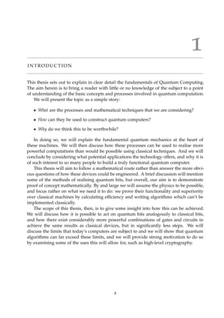
A C T I N G O N Q U B I T S
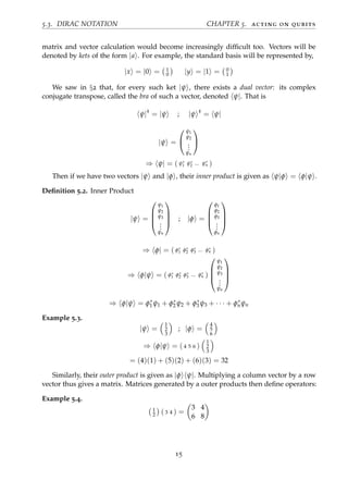
5.1 entanglement
Another unique property of quantum systems is that of entanglement: ie when two or
more particles interact in such a way that their individual quantum states can not be
described independent of the other particles. A quantum state then exists for the system
as a whole instead.
Mathematically, we consider such entangled states as those whose state can not be
expressed as a tensor product of the states of the individual qubits it’s composed of: they
are dependent upon the other.
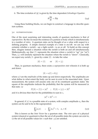
Example 5.1. Consider the state
|Φ+
=
1
√
2
[|00 + |11 ]
If we measure this state, we expect that it will be observed either as |00 or |11 , with
equal probability due to their equal magnitudes. The bases for this state are simply the
standard bases, |0 and |1 . Thus, according to our previous definition of systems of
multiple qubits, we would say this state can be given as a combination of two states
|Φ+
= |ψ1 ⊗ |ψ2
= [a1|0 + b1|1 ] ⊗ [a2|0 + b2|1 ]
= a1a2|00 + a1b2|01 + b1a2|10 + b1b2|11
However we require |Φ+ = 1√
2
[|00 + |11 ], which would imply a1b2 = 0 and b1a2 = 0.
These imply that either a1 = 0 or b2 = 0, and also that b1 = 0 or a2=0, which are
obviously invalid since we require that a1a2 = b1b2 = 1√
2
. Thus, we cannot express
|Φ+
= |ψ1 ⊗ |ψ2
and this is what we term an entangled state.
13](https://image.slidesharecdn.com/b93d7c4e-484e-4e7c-9a0b-90813b0817a5-160722100840/85/Mathematical_Introduction_to_Quantum_Computation-18-320.jpg)


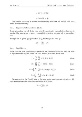

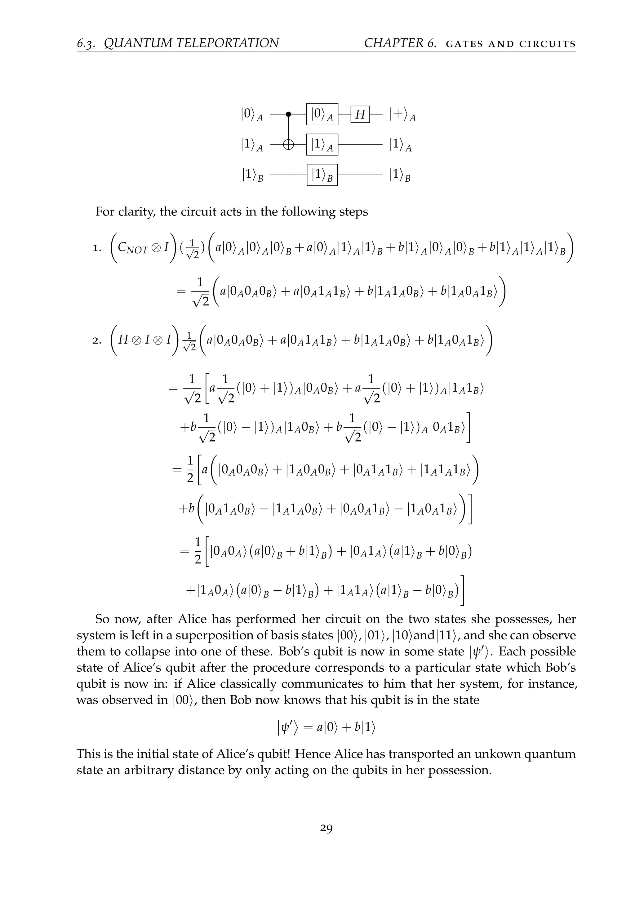
![6.3. QUANTUM TELEPORTATION CHAPTER 6. gates and circuits
So if A had been |0 and is now |1 , B gets flipped. If A had been |1 and is therefore now
|0 , B does not get flipped. Finally, step 3 returns A to its original value by performing
another NOT operation only on the first qubit. This is equivalent to a controlled-NOT
gate whose criteria is the control-bit being in state |0 initially.
So we can show this on a diagram as below. In diagrams such as this, a wire (qubit)
without any operation acting directly on it indicates the identity operator being imposed
on that qubit at that juncture. That is, it is equivalent to have an identity gate, I, as below
the first X-gate, as it is to have no gate there at all, as below the second X-gate here:
A X • X A
B I B ⊕ A ⊕ 1
6.2.3 Universal Gate Set
While this example is trivial, the principle is the same as it would be for any quantum
circuit. We can build circuits of arbitrary complexity using the ideas described so far. It
remains to define a set of gates which may be used to construct any circuit. We may do
so by recalling from § 5.2 that any quantum operation can be achieved by some unitary
transformation. Then, any unitary transformation may be achieved by a sequence of
simple quantum gates and quantum controlled-NOT gates. We will therefore take as a
universally approximating gate set, the generic set below, with U any unitary operation.
UG = {CNOT , U | U = U†
}
We will therefore proceed by constructing any operation we require provided they
are achievable by some combination of operations Oi,
O1O2 . . . On ; Oi ∈ UG
In most cases, circuits will be composed of the simple single qubit gates described al-
ready, put together to become multiple-qubit circuits, then used within quantum sub-
routines and algorithms.
6.3 quantum teleportation
We will now pause for a brief aside, in order to explore a more general concept of inter-
est in Quantum Information Theory, to appreciate the power of quantum mechanics. It can
be proven using only knowledge described so far, that it is possible to regenerate a quan-
tum state by transferring only classical information about the state [8]. An important
principle in quantum mechanics is that an unknown quantum state cannot be copied or
cloned [9]. Thus if we have an unkown superposition state |ψ = a0|0 + b0|1 , and an
auxiliary qubit |0 , onto which we hope to create a qubit, measurement upon which will
27](https://image.slidesharecdn.com/b93d7c4e-484e-4e7c-9a0b-90813b0817a5-160722100840/85/Mathematical_Introduction_to_Quantum_Computation-32-320.jpg)

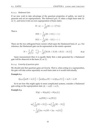
![6.3. QUANTUM TELEPORTATION CHAPTER 6. gates and circuits
There remains the cases where Alice observes her system in the other basis states,
however. Bob is still able to obtain the unkown state |ψ regardless of what measurement
Alice sees, by means of decoding his qubit. For example, had Alice measured |01 , then
Bob would know his qubit to be in the state a|1 + b|0 . To restore the initial amplitudes,
he must simply “swap” the states |0 ↔ |1 , which we know to be possible by the
quantum not gate, 6.1b. Likewise, he can restore |ψ by performing the Pauli-Y gate,
6.1c if Alice’s qubits had been in |11 , and by a Pauli-Z gate, 6.1d, if Alice’s is in |10 .
Example 6.7 (Decoding). If Alice had observed |10 , Bob then knows he has the state
|ψ = a|0 − b|1 . Bob would find the original qubit |ψ by implementing a Pauli-Z
gate:
Z ψ = |0 0| − |1 1| a|0 − b|1
= a|0 ( 0|0 ) − a|0 ( 0|1 ) − b|1 ( 1|0 ) + b|1 ( 1|1 )
= a|0 (1) − a|0 (0) − b|1 (0) + b|1 (1)
= a|0 + b|1
= |ψ
This is a simple of example of encrypting and decrypting messages. Quantum Infor-
mation theory builds on these ideas to consider how communication can be achieved
through quantum methods. Improvements offered over classical communication chan-
nels are of the same magnitude as the improvements quantum computation offers over
classical. This is explored in depth in a huge amount of literature on the subject, includ-
ing [7] and [10].
30](https://image.slidesharecdn.com/b93d7c4e-484e-4e7c-9a0b-90813b0817a5-160722100840/85/Mathematical_Introduction_to_Quantum_Computation-35-320.jpg)
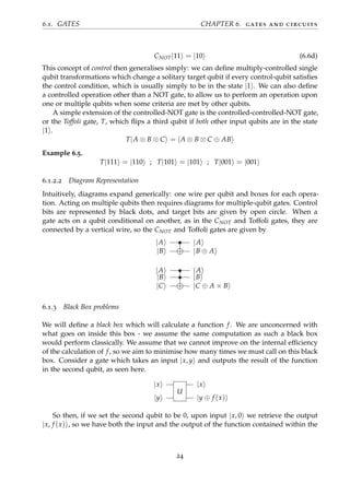
![7
C O M P U TAT I O N A L T E C H N I Q U E S
We have seen the equivalence of quantum gates and unitary operations, and we have
seen that any unitary operation is reversible in § 5.2. Thus any reversible gate is unitary.
We have also seen that it is possible to construct any unitary transformation using only
simple quantum gates, § 5.2.1. However, in general, such constructions are inefficient.
Quantum versions of classical computations are where efficiency may be improved upon
between the two cases: if we can define an efficient classical circuit, then build the
quantum version of this circuit by replacing all classical logic gates with simple quantum
gates, then we may begin to see where the power of quantum computation comes from.
Since we know we can build any unitary transformation using quantum gates, we can
replace any classical gate with a quantum analogue. However, classical circuits are not in
general reversible, so our problem is reduced to constructing reversible classical circuits,
but we also require that such gates be efficient, or else the procedure is redundant. An
in depth discussion of how this can be achieved is given in §6 of [11]. It will suffice for
our purposes to infer that if a reversible, classical gate can be achieved efficiently, then a
quantum analogue can be achieved trivially by replacing logic gates with their quantum
counterparts, which we have seen to exist already. We will instead explore algorithms
which make use of strictly quantum processes in order to achieve greater efficiency, and
compare such constructions with classical circuits that aim to do the same thing, so that
we can see the improvement offered.
7.1 techniques
With an understanding of how quantum circuits are constructed, we may now turn
to how their implementation can offer computational power. We will demonstrate a
simple proof of principle to see how quantum methods can achieve definitively superior
computational power, and we will outline some simple quantum subroutines which form
the basis of more complicated algorithms examined in the next chapter.
In doing so we will see the fundamental difference between classical and quantum
computation: it is by finding a global property of a function that we may solve it in
exponentially less steps. Quantum computers are uniquely capable of finding these
properties by working on superpositions to uncover information about a function, rather
than simply evaluating the function. This concept will become clearer in later quantum
computations, especially the algorithms for Simon’s problem, § 8.2.2, which finds the
31](https://image.slidesharecdn.com/b93d7c4e-484e-4e7c-9a0b-90813b0817a5-160722100840/85/Mathematical_Introduction_to_Quantum_Computation-36-320.jpg)
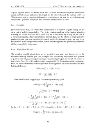
![7.1. TECHNIQUES CHAPTER 7. computational techniques
hidden variable of a function. It exploits the periodicity of a function, which Shor then
shows can be used to factor large integers, § 9. In doing so, these methods take a
property of the function, here the period, and use it to determine evaluations which
would be more difficult to achieve without knowing these properties.
We now consider the inapplicable problem designed by Deutsch to demonstrate
how properties of functions are achievable through quantum devices, in order to show,
through a simple example, the power of this idea.
7.1.1 Deutsch’s Problem
This proof by David Deutsch was the first concrete evidence that quantum methodology
can yield a result that would take a classical computer more steps [4]. The problem
addressed is of little practicality, though it is the conceptual proof we are interested in
here.
Recalling the black box (often referred to as an oracle) of § 6.1.3, we suppose that we
are interested in a function f : {0, 1} → {0, 1}. So our oracle now,
Uf : |x, y → |x, y ⊕ f (x)
We want to know if f (0) = f (1) or not. That is, whether the function returns a constant
answer for x ∈ {0, 1} or not. Define an system |+ |− by performing a Hadamard gate
on both qubits of the system |0 |1 , and use this as input to our oracle.
Uf |+ |− = Uf
1
2
(|0 + |1 )(|0 − |1 )
=
1
2
Uf |00 − |01 + |10 − |11
=
1
2
|0 |0 ⊕ f (0) − |0 |1 ⊕ f (0) + |1 |0 ⊕ f (1) − |1 |1 ⊕ f (1)
=
1
2
|0 |f (0) − |1 ⊕ f (1) + |1 |f (1) − |1 ⊕ f (1) (7.1)
=
1
2
1
∑
x=0
|x |0 ⊕ f (x) − |1 ⊕ f (x)
So now consider the quantity |0 ⊕ f (x) − |1 ⊕ f (x) .
|0 ⊕ f (x) − |1 ⊕ f (x) =
|0 ⊕ 0 − |1 ⊕ 0 = |0 − |1 =
√
2|− f (x) = 0
|0 ⊕ 1 − |1 ⊕ 1 = |1 − |0 = −
√
2|− f (x) = 1
= (−1)f (x)
√
2|−
32](https://image.slidesharecdn.com/b93d7c4e-484e-4e7c-9a0b-90813b0817a5-160722100840/85/Mathematical_Introduction_to_Quantum_Computation-37-320.jpg)

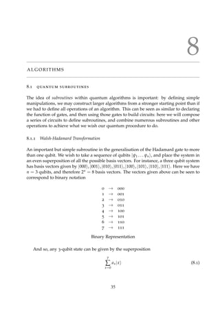

![8.1. QUANTUM SUBROUTINES CHAPTER 8. algorithms
+|01 . . . 00 + |01 . . . 10 + |01 . . . 01 + |01 . . . 11 + . . .
+|10 . . . 00 + |10 . . . 01 + |10 . . . 10 + |10 . . . 11 + . . .
+|11 . . . 00 + |11 . . . 01 + |11 . . . 10 + · · · + |11 . . . 11
Again, let the above basis states be considered binary for the numbers ( 0 → N − 1), and
this can be described by
1
√
N
N−1
∑
y=0
|y
We call this general operation the Walsh-Hadamard transformation [12]. When it acts
on on a system of n unentangled qubits, all initialised to |0 and therefore denoted |0 ⊗n
,
W(|0 ⊗n
) =
1
√
2n
2n−1
∑
y=0
|y (8.3)
More generally, consider the case where not all qubits in a system are initially |0 .
Suppose we have |z = |z0, z1, z2, ..., zn , then there exists |y = |y0, y1, ..., yn . Then z · y
is the number of common bits in z and y. For example, if |z = |0011 and |y = |1110 ,
then only the third entry is the same in both, so z · y = 1. Now, |z is a representation of
|z = |z0 ⊗ |z1 ⊗ ... ⊗ |zn
So let zi ∈ {0, 1} and compute
W|z = (H ⊗ H ⊗ H ⊗ · · · ⊗ H)(|z0 ⊗ |z1 ⊗ ... ⊗ |zn )
= (H|z0 ) ⊗ (H|z1 ) ⊗ · · · ⊗ (H|zn )
=
1
√
2n
(|0 + (−1)z0 |1 ) ⊗ (|0 + (−1)z1 |1 ⊗ · · · ⊗ (|0 + (−1)zn
|1 )
Again we will prove a simplified case and assume the generalisation as trivial. Consider
n = 3.
=
1
√
8
|0 + (−1)z0 |1 ⊗ |0 + (−1)z1 |1 ⊗ |0 + (−1)z2 |1 = |000 + (−1)z2 |001 + (−1)z1 |010
+(−1)z0 |100 + (−1)(z0+z2)
|101 + (−1)(z0+z1)
|110 + (−1)(z0+z1+z3)
|111 (8.4)
And as this is an evenly distributed three-qubit state, we can represent it as a sum
over basis states, given by
1
√
8
8
∑
y=0
|y =
1
√
8
|000 ± |001 ± |010 ± |011 ± |100 ± |101 ± |110 ± |111 (8.5)
37](https://image.slidesharecdn.com/b93d7c4e-484e-4e7c-9a0b-90813b0817a5-160722100840/85/Mathematical_Introduction_to_Quantum_Computation-42-320.jpg)
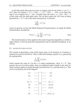
![8.2. QUANTUM PARALLELISM CHAPTER 8. algorithms
It is incorrect to think that, because a quantum process generates and works on the
superposition 1√
N
∑N
x=0 |x, f (x) , that a quantum computer can simply calculate and out-
put all possible results in one step. While it works on the superposition across the state
space of solutions of f (x), we must note that measurement of an n-qubit system will
only give one result. This is the same level of efficiency as a classical algorithm which
simply calculates f (x) for one x at a time. It is through methods as outlined above,
§ 7.1.1, that we may exploit quantum mechanics: rather than compute all solutions in
very few steps and then measure them, we must find a property common to all values
of f (x), and use it to work our way backwards to find a solution. This idea is utilised
in many quantum subroutines, including Simon’s Problem, which finds the period of a
function, and in more applicable complete algorithms, most famously Shor’s Algorithm,
which uses the period of a generated function to obtain prime factors of a number. We
will explore this algorithm fully in § 9.
8.2.1 Deutsch-Jozsa Problem
As another demonstration of generalising specific problems addressed, we will compose
a multiple qubit generalisation of Deutsch’s Problem, § 7.1.1. This is an improved version
of the above process, given 7 years later by [5]. We again consider a function f : Z2n → Z2
i.e that x ∈ X = {0, ..., 2n − 1} and f (x) ∈ {0, 1}.The function is known to be one of two
types: it will either be constant, always returns 0 or 1, or balanced, returns 0 exactly half
the time and 1 the other half. Our aim is to determine which of these types of function f
is. Again we have a quantum oracle Uf : |x |y → |x |y ⊕ f (x) . Through parallelisation,
we are working with the superposition
|ψ =
1
√
N
N
∑
x=0
|x (8.7)
We must note that it is possible to change the phase of a basis state depending on
some criteria of our choosing (see §7.4.2 of [11]). For our purpose, suppose there is a
subset X0 ∈ X, such that {f (xi) = 1|xi ∈ X0}. We change the phase for such vectors by a
global phase, a physically meaningless constant. In this case, the phase change we choose
is (−1). In other words, we have sent
|xi → −|xi = (−1)f (xi)
|xi
And applying this phase change throughout, 8.7 becomes
|ψ =
1
√
N
N
∑
x=0
(−1)f (x)
|x (8.8)
So for this problem then, we start with n qubits in the state |0 , and one in the state
|1 .
|ψ = |0 ⊗n
|1
39](https://image.slidesharecdn.com/b93d7c4e-484e-4e7c-9a0b-90813b0817a5-160722100840/85/Mathematical_Introduction_to_Quantum_Computation-44-320.jpg)

![8.2. QUANTUM PARALLELISM CHAPTER 8. algorithms
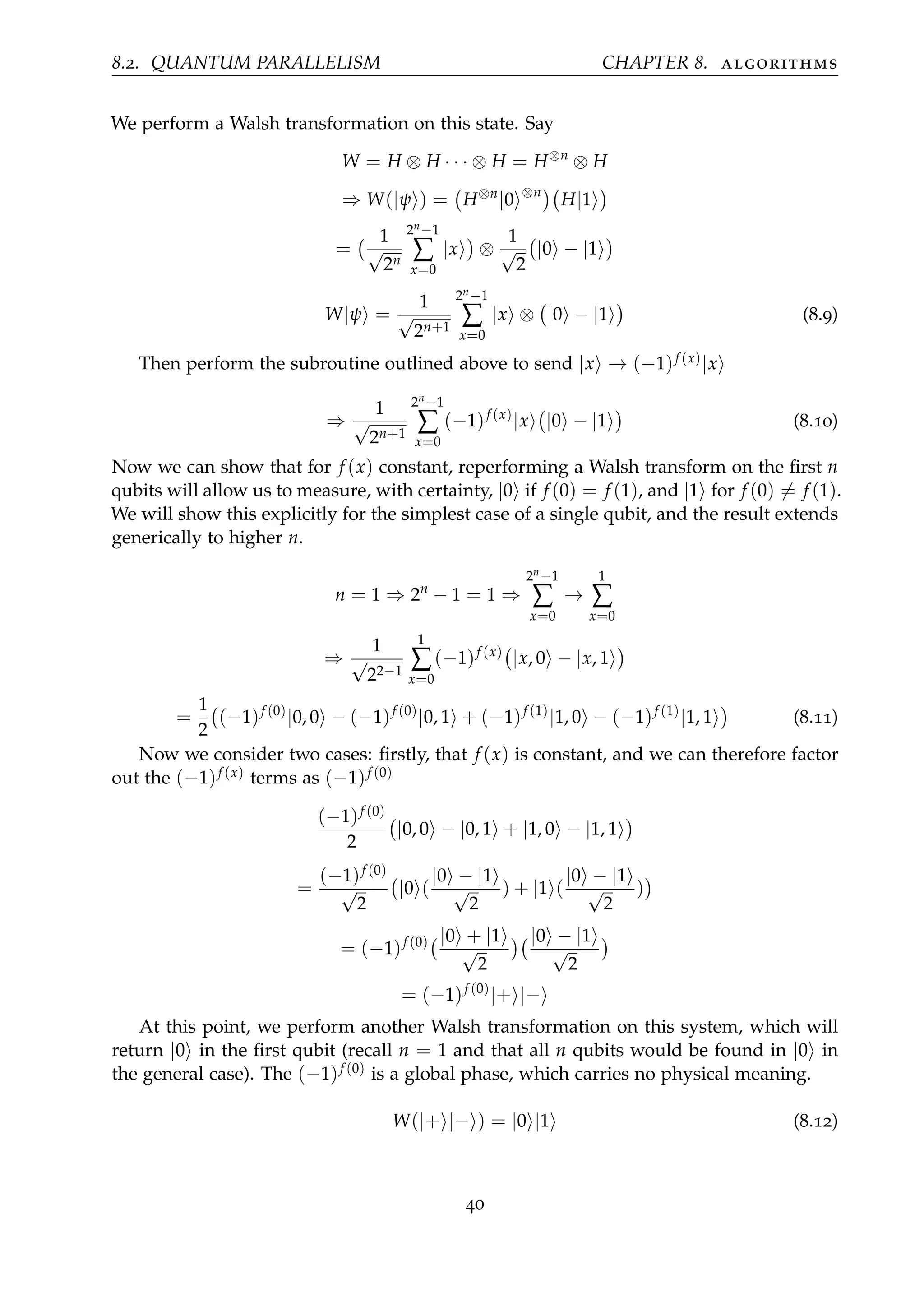
So with probability 1, if f (x) is constant, |0 will be measured in the first n qubits
following this procedure. Otherwise, in the case f (0) = f (1), the logic would change at
8.11:
1
2
(−1)f (0)
(|0, 0 − |0, 1 ) + (−1)f (1)
(|1, 0 − |1, 1 )
=
1
√
2
(−1)f (0)
|0 |− + (−1)f (1)
|1 |−
However, we know that either (f (0) = 0; f (1) = 1) or (f (0) = 1; f (1) = 0), and
substituting these would differ only by a constant, −1, so we can use the substitution
f (0) = 0; f (1) = 1, giving
(−1)f (0)
= (−1)0
= +1, (−1)f (1)
= (−1)1
= −1
⇒
1
√
2
|0 |− + (−1)|1 |−
=
|0 − |1
√
2
|− = |− |− (8.13)
And again we apply the Walsh tranform
W(|− |− ) = |1 |1
And so we can see clearly that, if f (0) = f (1), that, with probability 1, following the
Deutsch-Josza algorithm the first n qubits will be observed in the state |1 .
This algorithm has solved a problem with effectively no application, but it has proven
that there is a solution to this problem which requires only a single call to the oracle.
Comparatively, for a classical machine to find this result deterministically, it would require
at least 2n−1 + 1 calls to find the same result with certainty.
8.2.2 Simon’s Problem
Simon’s Problem addresses a function f with f (x) = f (x ⊕ a), (here ⊕ denotes modulus-
a addition), and aims to determine what value of a satisfies this [13]. In other words,
Simon’s Algorithm find the period of a function f. We focus on this particular subroutine
rather than the many others because it was this routine which suggested to Shor that
factorisation of large integers could be achieved by quantum computers in reasonable
time limits.
An initial state is generated by quantum parallelisation
2n−1
∑
x=0
|x |f (x) = ∑|ψ |φ
Where we have denoted the register of qubits holding initial values x as |ψ and the
register holding the values after evaluation in f as |φ . We know that f (x) = f (x ⊕ a)
41](https://image.slidesharecdn.com/b93d7c4e-484e-4e7c-9a0b-90813b0817a5-160722100840/85/Mathematical_Introduction_to_Quantum_Computation-46-320.jpg)

![9
S H O R ’ S A L G O R I T H M
Providing concrete examples of what only quantum machines can achieve is pivotal to
justifying funding research into their construction. We will outline the major driving
factor to date in quantum computation, factorisation of large numbers, described by
Shor’s Algorithm, to see one such example.
The aim of the algorithm is to factor large numbers, which is known to be extremely
difficult to achieve classically, [14]. To do so, we describe first the reasons that this can be
seen as a worthwhile driving force for research into quantum computation by outlining
how cryptography currently works. To describe mathematically how quantum methods
can uniquely be used in this area, we briefly discuss Fourier transforms and how they
can be translated into Quantum Fourier Transforms. To realise the potential application
of quantum mechanics, we will reduce the problem of factoring a large number to that
of finding the period of a function we can generate based on the number we wish to
factorise, and then show how we may find such a period only through manipulation
of quantum states. True quantum mechanics will play only a minor role insofar as it
will be used in very few steps of the algorithm, but by doing so we will see how and
why classical computation could never achieve the same efficiency as we will find for
quantum computation.
9.1 cryptography
Current encryption relies on the principle that it is very easy to multiply two large primes
together to form a semi-prime number, while it is extremely difficult to factor a semi
prime into its two factors. Multiplying two prime numbers of the order 10100 will result
in a number of order 10200, which is extremely hard to factor classically. Encryption
therefore generates a public key, the product of the primes, and a private key, the numbers
used to generate it, known only to those who need to know how to decrypt the message.
For this reason, Shor’s factoring algorithm poses a threat to standard cryptography at
present, as it would drastically simplify the process of decoding the secret key, and
would thus render currently secure communications as potentially insecure, [15]. This
is a detractor for the field of study, though it is seen as a turning point in quantum
computing insofar as it sparked huge interest in the subject immediately following the
publication of the original paper, [6]. It is a fundamental concept to the subject, so
45](https://image.slidesharecdn.com/b93d7c4e-484e-4e7c-9a0b-90813b0817a5-160722100840/85/Mathematical_Introduction_to_Quantum_Computation-50-320.jpg)

![9.3. FACTORISATION BY PERIOD FINDING CHAPTER 9. shor’s algorithm
= 1 + (−1)(−1)
1
2 + (−1) + (−1)4
(−1)
1
2
= 1 − i − 1 + i = 0
Any other value of x that isn’t an integer multiple of N
r will demonstrate this behaviour
and sum to zero. This behaviour extends to larger values of n and R such that we can
say that the only Fourier coefficients which are non zero are F(x = k N
r ), k ∈ N. In this
case, the state after QFT is a superposition of |0 and |4 :
F(0)|0 + F(1)|4 = F(0) 0(
N
r
) + F(1) 1(
N
r
)
Now that we know that the only nonzero Fourier coefficients correspond to x being
a multiple of N
r we can say that the state after Fourier transformation
F(x)|x
can only be measured to exist for such values of x. So then, if measured, the observed
value would be some k N
r . The state after performing the QFT is given by
QFT(f (x)) =
r−1
∑
k=0
F(k) k(
N
r
) (9.4)
Producing this state is the most important quantum subroutine used in quantum
computation, and we will see its use in Shor’s Algorithm. The realisation of the QFT is
explained in §7.8 of [11], which builds on the earlier idea of defining relatively simple
gates and combining them recursively.
9.3 factorisation by period finding
Recall our overall aim here: we wish to factor an integer, M, into its prime factors, mi.
For example, M = 21 = m1 × m2 = 7 × 3. Using modular addition, we define any
integer as a mod M, e.g to define 30, we say 30mod21 ≡ 9mod21. We define the order of
such an integer as the first r which satisfies
ar
− 1 ≡ 0mod M (9.5)
Example 9.1. If we consider M = 7 and we wish to find the order of a = 2, we are
considering integers
a mod M ≡ 2mod 7, 9mod 7, 16 mod 7, ...
. We have
p mod 7 ≡ 0 for p = 7, 14, 21, 28, ...
So we are looking for the lowest value of r for each a to give ar − 1 = 7k where k ∈ N.
48](https://image.slidesharecdn.com/b93d7c4e-484e-4e7c-9a0b-90813b0817a5-160722100840/85/Mathematical_Introduction_to_Quantum_Computation-53-320.jpg)

![9.4. STEPS OF SHOR’S ALGORITHM CHAPTER 9. shor’s algorithm
9.4 steps of shor’s algorithm
We are now in a position to describe the steps taken in Shor’s Algorithm to factor an
integer M into its prime factors. A preliminary to the algorithms is deciding how many
qubits to compose the system of. It can be shown (§8.3, [11]) that the number of qubits,
n, should be chosen to satisfy
M2
≤ 2n
≤ 2M2
(9.6)
We will do so a number of times. First, we will go through each step in explicit detail
and explain the concepts involved. Then, we will succinctly summarise the steps. Finally,
we will walk through the programme precisely for a specific value to be factorised.
9.4.1 Detailed Description of Steps
1. Randomly choose a value for a that is relatively prime to M. (If they are not
relatively prime then a is a factor and the rest of the algorithm is redundant, so it
is necessary to check this condition early by a simple Euclidean algorithm).
2. Since we are interested in the function f (x) = ax mod M, we generate it within the
superposition of an n-qubit state obtained through quantum parallelisation (recall
§ 8.2), by passing a register of qubits |x together with a register of |0 ’s through a
parallelisation scheme, giving the output
1
√
2n
2n−1
∑
x=0
|x |f (x) =
1
√
2n
2n−1
∑
x=0
|x |ax
modM (9.7)
Since our function is periodic in r, f (x) = f (x + r), we saw in 8.2.2 that measuring
only the second register would place the first register into a superposition over
some x0 and x0 + l.r, l ∈ Z, where the second register was observed in |f (x0) . We
introduce a function, g(x), to determine whether each x is separated from x0 by
the period or not:
g(x) =
1 f (x) = f (x0) , (x = x0 + l.r)
0 f (x) = f (x0) , (x = x0 + l.r)
After measurement of the second qubit, our system is in the state
C ∑
x
g(x) |x |f (x0) (9.8)
Where C is a scaling factor.
3. Since the two registers are not entangled, we can safely ignore the register that
holds f (x), and focus solely on the state
C ∑
x
g(x) |x (9.9)
50](https://image.slidesharecdn.com/b93d7c4e-484e-4e7c-9a0b-90813b0817a5-160722100840/85/Mathematical_Introduction_to_Quantum_Computation-55-320.jpg)
![9.4. STEPS OF SHOR’S ALGORITHM CHAPTER 9. shor’s algorithm
Applying the Quantum Fourier Transform, 9.4:
QFT C ∑
x
g(x)|x = C2
r−1
∑
k=0
G(k) k(
N
r
) (9.10)
Where C2 is another scaling constant. g(x) has the same period, r, as f (x) and G(x)
is the Fourier coefficient for g(x), given by 9.1.
4. The above assumes that N = 2n and r = 2R. In the case that r = 2R, the transform
approximates the exact case: most of the amplitude is associated with integers
equal to or near a multiple of the ratio N
r . In this way, following this procedure,
were we to measure the system, with high probability we can say that the observed
value for x is a multiple of N
r , or else a value very near to it. Assign the measure-
ment found in this step the label β.
5. Having obtained a β, use the purely classical procedure of continued fractions to
deduce the period r. We have obtained a measurement from step 4 which we are
confident generates an integer near to a multiple of N
r , (given by β = jN
r + ε, where
ε is small compared with N). We are interested in finding r. We know N = 2n, so
if we consider the fraction
β
N
= j
N
r
1
N
+
ε
N
=
j
r
+
ε
N
In the simplest case, r = 2R, so ε = 0, and this means that simply reducing the
fraction
β
N yields a fraction which we can see as being
j
r , and we can read the
denominator as the period r we’re interested in. In general, this is not the case,
so we must consider ε = 0. In this case we apply the method of continuously
expanding fractions. This is a purely classical mathematical argument, examined
well by much of the literature on this topic, for instance in [16].
β
N
=
j
r
+
ε
N
By fraction expansion, we may continuously change the fraction
β
N to reflect a
significant fraction,
j
r with some small correction, ε
N . We aim to calculate the signif-
icant fraction and use it to read the denominator as the period r. We require that
r < M, so we terminate the procedure when the denominator of our ”significant”
fraction exceeds M.
A general fraction expansion is given by
A
B
= a0 +
1
a1 + 1
a2+ 1
...+ 1
ap
(9.11)
51](https://image.slidesharecdn.com/b93d7c4e-484e-4e7c-9a0b-90813b0817a5-160722100840/85/Mathematical_Introduction_to_Quantum_Computation-56-320.jpg)
![9.4. STEPS OF SHOR’S ALGORITHM CHAPTER 9. shor’s algorithm
This is represented by A
B = [a0; a1, a2, ..., ap]. The the qth convergent is an approxima-
tion for A
B given by [a0, a1, ..., aq] for any 0 ≤ q ≤ p. For instance,
85
70
= [1; 4, 1, 2] = 1 +
1
4 + 1
1+ 1
1+ 1
2
= 1.214286
And if we take q1 corresponding to approximation using only one fraction, q1 =
[1; 4], we would find
83
70
≈ q1 = [1; 4] = 1 +
1
4
=
5
4
=
q1,num
q1,den
Which is a fair approximation.
⇒
85
70
= 1.214286 =
5
4
− 0.035714
If we consider q2 = [1; 4, 1]
q2 = 1 +
1
4 + 1
1
= 1 +
1
5
=
6
5
= 1.2
⇒ 1.214286 =
6
5
+ 0.014286
So we can see that every time we boil the fraction down to the next value of q, the
dominant fraction gets closer to the actual value and the correction becomes very
small.
We are trying to generate a guess for our period r, but r < M, so we are only
interested in denominators of qi which are less than M. If we say qi =
qi,num
qi,den
, we
look for the first such qi,den to satisfy (qi,den < M < qi+1,den), and we try to complete
the algorithm using r = qi,den.
Now, if we apply this to our situation: we have measured a β which we know to
be near a multiple of N
r . Take an explicit example, say N = 512 = 210, and that we
are trying to factor M = 21. Suppose the output of the quantum implementation
is β = 89.
β
N
=
89
512
= 0.173823 = [0; 5, 1, 3, 22]
= 0 +
1
5 + 1
1+ 1
3+ 1
22
We calculate the values for qi
q0 = [0] = 0
52](https://image.slidesharecdn.com/b93d7c4e-484e-4e7c-9a0b-90813b0817a5-160722100840/85/Mathematical_Introduction_to_Quantum_Computation-57-320.jpg)
![9.4. STEPS OF SHOR’S ALGORITHM CHAPTER 9. shor’s algorithm
q1 = [0; 5] = 0 +
1
5
= 0.2
q2 = [0; 5, 1] = 0 +
1
5 + 1
1
=
1
6
= 0.16667
q3 = [0; 5, 1, 3] = 0 +
1
5 + 1
1+1
3
=
1
5 + 4
3
=
1
23
4
=
4
23
= 0.173913
q4 = [0; 5, 1, 3, 22] = 0 +
1
5 + 1
1+ 1
3+ 1
22
=
89
512
= 0.173823
Clearly, the highest qi,den < M is
(q2,den = 6) < (M = 21) < (23 = q3,den)
Thus we take r = 6 as our period and try to complete the algorithm using this.
One way to think of this is as
β =
j
r
+
ε
N
= α
j
r
In our particular example, r = 6 and
β = 89 = 1(
512
6
) + 3.67
so j = 1.
β
N
=
89
512
= 0.173828 = α0
1
6
⇒ α0 = 1.042969
After the first expanded fraction we said that q1 = [0; 5]
⇒
89
512
= 0 +
1
5
= 0.2 = α1
j
r
= α1
1
6
⇒ α1 = 1.2
Taking q2 = [0; 5, 1]
89
512
= 0 +
1
5 + 1
1
=
1
6
= α2
1
6
⇒ α2 = 1
Note this is the case we’re looking for; we’ve boiled
β
N down to
j
r . We now need to
know when we’ve gotten to this point in general.
q3 = [0; 5, 1, 3] = 0 +
1
5 + 1
1+1
3
=
4
23
= α3
1
6
⇒ α3 =
24
23
At the point where the denominator of qi exceeds M, we must have passed the case
where the denominator was the period r, since r < M, so we can read r from the
denominator of qi.
6. When r is odd, return to the start of the procedure using a different value for a.
7. When r is even, use a Euclidean algorithm to determine whether either of (a
r
2 + 1)
or (a
r
2 − 1) share a non-trivial factor with M. If so, we have found a factor of M.
53](https://image.slidesharecdn.com/b93d7c4e-484e-4e7c-9a0b-90813b0817a5-160722100840/85/Mathematical_Introduction_to_Quantum_Computation-58-320.jpg)
![9.4. STEPS OF SHOR’S ALGORITHM CHAPTER 9. shor’s algorithm
with
g(x) =
1 x = x0 + l.r
0 x = x0 + l.r
We can now ignore the second register and focus only on the superposition
C
2047
∑
x=0
g(x)|x
3. Perform the quantum Fourier Transformation, yielding
QFT(C
2047
∑
x=0
g(x)|x ) = C2
r−1
∑
k=0
G(k)|k
4. Measure the system after this transformation. This will result in some β. Suppose
we measure β = 206.
5. Compute
β
N
=
206
2048
=
103
1024
By continued fraction expansion this can be represented by
103
1024
= 0 +
1
9 + 1
1+ 1
16+ 1
6
We calculate the values of q for this fraction
q0 = [0] = 0
q1 = [0; 9] =
1
9
q2 = [0; 9, 1] =
1
10
q3 = [0; 9, 1, 16] =
17
169
q4 = [0; 9, 1, 16, 6] =
103
1024
Considering the denominators of these shows that q2,den < M < q3,den holds:
10 < 35 < 169
So we proceed using r = q2,den = 10.
6. r is not odd, so we move to the next step.
55](https://image.slidesharecdn.com/b93d7c4e-484e-4e7c-9a0b-90813b0817a5-160722100840/85/Mathematical_Introduction_to_Quantum_Computation-60-320.jpg)
![9.5. EFFICIENCY IMPROVEMENT CHAPTER 9. shor’s algorithm
7. r is even, so we compute (a
r
2 ± 1)
(6
10
2 + 1) = (65
+ 1) = 7777
(6
10
2 − 1) = (65
− 1) = 7775
Then use the Euclidean algorithm to show that
m1 = gcd(7777, 35) = 7
m2 = gcd(7775, 35) = 5
Thus we have found 35 = m1.m2 = 7 × 5, and we can verify that, for this simple
case, the algorithm works.
It is worth noting here that the period of (f (x) = 6x mod 35) is in fact 2:
62
mod 35 ≡ 1
64
mod 35 ≡ 1
...
610
mod 35 ≡ 1
Yet the algorithm still worked and found the correct factorisation for 35.
9.5 efficiency improvement
In order that we can understand the improvement offered by Shor’s factoring algo-
rithm, we must consider how many steps it requires for its implementation, and
compare this with the number of steps a classical algorithm would take
9.5.1 Classical Factorisation
The general approach, [14], to finding a factor of M is to sequentially compute
M
1
,
M
2
,
M
3
, ... ,
M
√
M
In some cases, a suitable factor will appear very early in this procedure, but in
some cases it could take all
√
M attempts. On average, it is fair to say that it will
take
√
M
2 trials to identify a factor. Each iteration will have some time expense, we
will say as small as 10−12 seconds, so let us consider how many trials a realistic
problem would require and find how long it would take a classical computer to
solve this.
56](https://image.slidesharecdn.com/b93d7c4e-484e-4e7c-9a0b-90813b0817a5-160722100840/85/Mathematical_Introduction_to_Quantum_Computation-61-320.jpg)
![9.5. EFFICIENCY IMPROVEMENT CHAPTER 9. shor’s algorithm
Example 9.3. If the number we wish to factorise, M, has, for instance, 77 digits, we
can sat that is of the order 2256 since 2256 = 1.15 × 1077. Then
√
M ∼ (2256
)
1
2 = 2128
⇒
√
M
2
∼ (2128
)−1
= 2127
Trials
In time, this will take
2127
Trials × 10−12
seconds per Trial
∼ 1026
seconds
The universe is approximately 4 × 10¹⁷ seconds old, so obviously trying to factor
such a number is not achievable classically. The best known factoring algorithm,
the number field sieve, [17] offers an improvement over this time scale, but not by
nearly the same amount as the improvement offered by quantum computing, [18].
9.5.2 Quantum Factoring Algorithm
The most demanding part of the algorithm is the modular exponentiation required to
generate the calculation of f (x) = ax mod M inside the state. §6.4 of [11] discusses
this generation in detail, and Shor shows that it can be most efficiently achieved in
O(n2 log2 n log2 log2 n) time steps, where n is the number of qubits involved in
the system [19]. (Recall N = 2n)
Rieffel and Polak also discuss the number of steps required of each section of
the algorithm as outlined here, §8.4 of [11]. Clearly the most computationally
expensive calculation is that of modular exponentiation, which we have seen to
cost of the order (n2 log2 n log2 log2 n) in time.
Again aiming to factorise a number of the order 2256, we must first find what size
of a system (number of qubits) would be required. This is determined by
M2
≤ 2n
≤ 2M2
⇒ 2512
≤ 2n
≤ 2513
In general M will not be a power of two, and there will be only one such n to satisfy
this condition. It suffices here to choose n = 512. The majority of the computation
is due to the modular exponentiation, so we must calculate O(n2 log2 nlog2log2 n)
to get an idea of how many steps are needed.
n = 512 ⇒ log2n = log2(29
)
⇒ log2 n = 9
57](https://image.slidesharecdn.com/b93d7c4e-484e-4e7c-9a0b-90813b0817a5-160722100840/85/Mathematical_Introduction_to_Quantum_Computation-62-320.jpg)
![9.5. EFFICIENCY IMPROVEMENT CHAPTER 9. shor’s algorithm
⇒ log2 log2 n = log2(9) ≈ 3
⇒ n2
log2 n log2 log2 n = (512)2
× 9 × 3
= 7, 077, 888 Trials
⇒ Time = (7, 077, 888 Trials) × (10−12
seconds per Trial)
= 7 × 10⁻⁶
seconds
This is clear evidence that Shor’s Algorithm is definitively faster than any classical
algorithm can ever achieve.
Thus, we have given a concrete example of a case where quantum computing can
be implemented to solve a real problem which cannot be efficiently dealt with
by a classical computer. There are, however, many other promising applications,
such as the needle-in-the-haystack problem addressed by Grover’s Algorithm, [20].
There is potential to model quantum chemistry far more accurately than is done at
present by modelling chemical bonds at quantum levels through use of quantum
computation, [21]. Such modelling currently occupies a huge amount of computa-
tional resources worldwide in trying to achieve accurate models at quantum scales.
It is thought that quantum computers may be able to save resources and help in
the modelling of specific chemical bonds at quantum levels, [22], and therefore
help in the development of more effective medicines. These are only some of the
vast possible applications of the technology, and so it is clear that there is suffi-
cient motivation for the field to develop and to potentially shape the technological
landscape over the coming years and decades.
58](https://image.slidesharecdn.com/b93d7c4e-484e-4e7c-9a0b-90813b0817a5-160722100840/85/Mathematical_Introduction_to_Quantum_Computation-63-320.jpg)
![B I B L I O G R A P H Y
[1] Yu I Manin. Vychislimoe i nevychislimoe (computable and noncomputable),
moscow: Sov, 1980.
[2] Richard P Feynman. Simulating physics with computers. International journal of
theoretical physics, 21(6):467–488, 1982.
[3] Paul Benioff. Quantum mechanical hamiltonian models of turing machines. Journal
of Statistical Physics, 29(3):515–546, 1982.
[4] David Deutsch. Quantum theory, the church-turing principle and the universal
quantum computer. In Proceedings of the Royal Society of London A: Mathematical,
Physical and Engineering Sciences, volume 400, pages 97–117. The Royal Society, 1985.
[5] David Deutsch and Richard Jozsa. Rapid solution of problems by quantum compu-
tation. Proceedings of the Royal Society of London. Series A: Mathematical and Physical
Sciences, 439(1907):553–558, 1992.
[6] Peter W Shor. Algorithms for quantum computation: Discrete logarithms and fac-
toring. In Foundations of Computer Science, 1994 Proceedings., 35th Annual Symposium
on, pages 124–134. IEEE, 1994.
[7] Michael A Nielsen and Isaac L Chuang. Quantum computation and quantum informa-
tion. Cambridge university press, 2010.
[8] Charles H Bennett, Gilles Brassard, Claude Cr´epeau, Richard Jozsa, Asher Peres,
and William K Wootters. Teleporting an unknown quantum state via dual classical
and einstein-podolsky-rosen channels. Physical review letters, 70(13):1895, 1993.
[9] WK Wooters and WK Zurek. Quantum no-cloning theorem. Nature, 299:802, 1982.
[10] Mark M Wilde. Quantum information theory. Cambridge University Press, 2013.
[11] Eleanor G Rieffel and Wolfgang H Polak. Quantum computing: A gentle introduction.
MIT Press, 2011.
[12] Bernard J. Fino and V. Ralph Algazi. Unified matrix treatment of the fast walsh-
hadamard transform. IEEE Transactions on Computers, 25(11):1142–1146, 1976.
[13] Daniel R Simon. On the power of quantum computation. SIAM journal on computing,
26(5):1474–1483, 1997.
[14] John M Pollard. A monte carlo method for factorization. BIT Numerical Mathematics,
15(3):331–334, 1975.
[15] Isaac Chuang, Raymond Laflamme, P Shor, and W Zurek. Quantum computers,
factoring, and decoherence. arXiv preprint quant-ph/9503007, 1995.
[16] C Lavor, LRU Manssur, and R Portugal. Shor’s algorithm for factoring large integers.
arXiv preprint quant-ph/0303175, 2003.
60](https://image.slidesharecdn.com/b93d7c4e-484e-4e7c-9a0b-90813b0817a5-160722100840/85/Mathematical_Introduction_to_Quantum_Computation-65-320.jpg)
![BIBLIOGRAPHY BIBLIOGRAPHY
[17] Arjen K Lenstra, Hendrik W Lenstra Jr, Mark S Manasse, and John M Pollard. The
number field sieve. Springer, 1993.
[18] Shah Muhammad Hamdi, Syed Tauhid Zuhori, Firoz Mahmud, and Biprodip Pal.
A compare between shor’s quantum factoring algorithm and general number field
sieve. In Electrical Engineering and Information & Communication Technology (ICEEICT),
2014 International Conference on, pages 1–6. IEEE, 2014.
[19] Peter W Shor. Polynomial-time algorithms for prime factorization and discrete log-
arithms on a quantum computer. SIAM journal on computing, 26(5):1484–1509, 1997.
[20] Lov K Grover. A fast quantum mechanical algorithm for database search. In Pro-
ceedings of the twenty-eighth annual ACM symposium on Theory of computing, pages
212–219. ACM, 1996.
[21] Benjamin P Lanyon, James D Whitfield, GG Gillett, Michael E Goggin, Marcelo P
Almeida, Ivan Kassal, Jacob D Biamonte, Masoud Mohseni, Ben J Powell, Marco Bar-
bieri, et al. Towards quantum chemistry on a quantum computer. Nature Chemistry,
2(2):106–111, 2010.
[22] Christof Zalka. Simulating quantum systems on a quantum computer. Proceedings
of the Royal Society of London. Series A: Mathematical, Physical and Engineering Sciences,
454(1969):313–322, 1998.
61](https://image.slidesharecdn.com/b93d7c4e-484e-4e7c-9a0b-90813b0817a5-160722100840/85/Mathematical_Introduction_to_Quantum_Computation-66-320.jpg)


![1.1. MOTIVATION CHAPTER 1. introduction
1.1 motivation
Since the notion of a quantum computer was first suggested by Yuri Manin in 1980 [1],
and seperately by Richard Feynman [2], many prominent mathematicians and physicists
have studied the topic in great depth. In 1982, the first potential framework of a quantum
computer was proposed by Paul Benioff [3]. In the following years, it was proven that
there were processes for which quantum computing could be shown to out-perform its
classical counterpart, in particular by the work of David Deutsch, [4]. In 1992, Deutsch,
together with Richard Josza released a paper entitled Rapid solution of problems by quan-
tum computation, in which they showed how quantum machines could be used to achieve
exponential speed-up in solving computational problems [5]. The problems that their al-
gorithm was able to solve, however, were of little practical use, so there was no known
reason to actually invest in the construction of such potentially useless devices. In 1994,
Peter Shor published a paper that became a turning point in the history of quantum
computing: his now-famous algorithm used techniques only available to quantum com-
puters to solve factorisation problems. He showed that a quantum computer would be
able to factorise large numbers with significantly less computational expense than clas-
sical machines will ever be capable of [6]. Following this milestone, it became clear that
quantum methods have the capacity to transcend classical machines, and so the field has
been growing steadily as a research topic since.
In the late 1990’s, the first quantum computer was built utilising 2 qubits. There have
been significant strides every year since then towards a fully functional model.
Thus our motivation is clear: the entire quantum computing industry is built on the
belief that, quite soon, we will be able to build computers which operate at exponen-
tially faster and more efficient rates than we will ever be able to achieve using classical
implementations.
We endeavour to understand the building blocks which are at the centre of this po-
tentially massive transition to a new kind of computation.
3](https://image.slidesharecdn.com/b93d7c4e-484e-4e7c-9a0b-90813b0817a5-160722100840/75/Mathematical_Introduction_to_Quantum_Computation-8-2048.jpg)
![2
L I N E A R A L G E B R A
Before getting too involved in mechanical view points and quantum physics, it is im-
portant to review the language with which these topics will be discussed: here we will
recap some basics of linear algebra and summarise the basic mathematical techniques
required to describe physics at a quantum scale.
2.1 recap of basics
Some algebraic knowledge is assumed of the reader. For further discussion and deriva-
tion of some points, consult §2.1 of the standard text on the subject on quantum comput-
ing and information processing, Nielsen and Chuang. [7]. We will briefly recall some
definitions for reference.
• Notation
Definition of Representation
Vector (or ket) |ψ
Dual Vector (or bra) ψ|
Tensor Product |ψ ⊗ |φ
Complex conjugate |ψ∗
Transpose |ψ T
Adjoint |ψ †
= (|ψ ∗
)T
Algebraic Definitions
The dual vector of a vector (ket) |ψ is given by ψ| = |ψ †
. The adjoint of a matrix
replaces each matrix element with its own complex conjugate, and then switches
its columns with rows.
M†
=
M0,0 M0,1
M1,0 M1,1
†
=
M∗
0,0 M∗
0,1
M∗
1,0 M∗
1,1
T
=
M∗
0,0 M∗
1,0
M∗
0,1 M∗
1,1
(2.1)
5](https://image.slidesharecdn.com/b93d7c4e-484e-4e7c-9a0b-90813b0817a5-160722100840/75/Mathematical_Introduction_to_Quantum_Computation-10-2048.jpg)


![4.3. MULTIPLE QUBITS CHAPTER 4. quantum bits
Consider first a simple system of 2 qubits. Measuring in the standard basis, these
qubits will have to collapse in to one of the basis states |0, 0 , |0, 1 , |1, 0 , |1, 1 . Thus, for
such a 2-qubit system, we have the general superposition
|ψ = α0,0|0, 0 + α0,1|0, 1 + α1,0|1, 0 + α1,1|1, 1
where αi,j is the amplitude for measuring the system as the state |i, j . This is perfectly
analogous to a classical 2-bit system necessarily occupying one of the four possibilities
(0, 0), (0, 1), (1, 0), (1, 1).
Hence, for example, if we wanted to concoct a two-qubit system composed of one
qubit in the state |+ and one in |−
|ψ = |+ ⊗ |−
|ψ = (
1
√
2
|0 +
1
√
2
|1 ) ⊗ (
1
√
2
|0 −
1
√
2
|1 )
=
1
2
[|00 − |01 + |10 − |11 ]
=
1
2
1
0 ⊗ 1
0 − 1
0 ⊗ 0
1 + 0
1 ⊗ 1
0 − 0
1 ⊗ 0
1
=
1
2
1
0
0
0
−
0
1
0
0
+
0
0
1
0
−
0
0
0
1
|ψ =
1
2
1
−1
−1
1
That is, the system is given by a linear combination of the four basis vectors
1
0
0
0
,
0
1
0
0
,
0
0
1
0
,
0
0
0
1
We can notice that a single qubit system can be described by a linear combination of two
basis vectors, and that a two qubit system requires four basis vectors to describe it. In
general we can say that an n-qubit system is represented by a linear combination of 2n
basis vectors.
4.3.1 Registers
A register is the name given to a system of multiple qubits. We may use the idea to
consider a system of n qubits as two sub systems. For instance, a register of ten qubits
can be denoted |x[10] , and we can think of the system as a register of six qubits together
with a register of three and another register of one qubit.
|x[10] = |x1[6] ⊗ |x2[3] ⊗ |x3[1]
12](https://image.slidesharecdn.com/b93d7c4e-484e-4e7c-9a0b-90813b0817a5-160722100840/75/Mathematical_Introduction_to_Quantum_Computation-17-2048.jpg)
![5
A C T I N G O N Q U B I T S
5.1 entanglement
Another unique property of quantum systems is that of entanglement: ie when two or
more particles interact in such a way that their individual quantum states can not be
described independent of the other particles. A quantum state then exists for the system
as a whole instead.
Mathematically, we consider such entangled states as those whose state can not be
expressed as a tensor product of the states of the individual qubits it’s composed of: they
are dependent upon the other.
Example 5.1. Consider the state
|Φ+
=
1
√
2
[|00 + |11 ]
If we measure this state, we expect that it will be observed either as |00 or |11 , with
equal probability due to their equal magnitudes. The bases for this state are simply the
standard bases, |0 and |1 . Thus, according to our previous definition of systems of
multiple qubits, we would say this state can be given as a combination of two states
|Φ+
= |ψ1 ⊗ |ψ2
= [a1|0 + b1|1 ] ⊗ [a2|0 + b2|1 ]
= a1a2|00 + a1b2|01 + b1a2|10 + b1b2|11
However we require |Φ+ = 1√
2
[|00 + |11 ], which would imply a1b2 = 0 and b1a2 = 0.
These imply that either a1 = 0 or b2 = 0, and also that b1 = 0 or a2=0, which are
obviously invalid since we require that a1a2 = b1b2 = 1√
2
. Thus, we cannot express
|Φ+
= |ψ1 ⊗ |ψ2
and this is what we term an entangled state.
13](https://image.slidesharecdn.com/b93d7c4e-484e-4e7c-9a0b-90813b0817a5-160722100840/75/Mathematical_Introduction_to_Quantum_Computation-18-2048.jpg)


![6.3. QUANTUM TELEPORTATION CHAPTER 6. gates and circuits
So if A had been |0 and is now |1 , B gets flipped. If A had been |1 and is therefore now
|0 , B does not get flipped. Finally, step 3 returns A to its original value by performing
another NOT operation only on the first qubit. This is equivalent to a controlled-NOT
gate whose criteria is the control-bit being in state |0 initially.
So we can show this on a diagram as below. In diagrams such as this, a wire (qubit)
without any operation acting directly on it indicates the identity operator being imposed
on that qubit at that juncture. That is, it is equivalent to have an identity gate, I, as below
the first X-gate, as it is to have no gate there at all, as below the second X-gate here:
A X • X A
B I B ⊕ A ⊕ 1
6.2.3 Universal Gate Set
While this example is trivial, the principle is the same as it would be for any quantum
circuit. We can build circuits of arbitrary complexity using the ideas described so far. It
remains to define a set of gates which may be used to construct any circuit. We may do
so by recalling from § 5.2 that any quantum operation can be achieved by some unitary
transformation. Then, any unitary transformation may be achieved by a sequence of
simple quantum gates and quantum controlled-NOT gates. We will therefore take as a
universally approximating gate set, the generic set below, with U any unitary operation.
UG = {CNOT , U | U = U†
}
We will therefore proceed by constructing any operation we require provided they
are achievable by some combination of operations Oi,
O1O2 . . . On ; Oi ∈ UG
In most cases, circuits will be composed of the simple single qubit gates described al-
ready, put together to become multiple-qubit circuits, then used within quantum sub-
routines and algorithms.
6.3 quantum teleportation
We will now pause for a brief aside, in order to explore a more general concept of inter-
est in Quantum Information Theory, to appreciate the power of quantum mechanics. It can
be proven using only knowledge described so far, that it is possible to regenerate a quan-
tum state by transferring only classical information about the state [8]. An important
principle in quantum mechanics is that an unknown quantum state cannot be copied or
cloned [9]. Thus if we have an unkown superposition state |ψ = a0|0 + b0|1 , and an
auxiliary qubit |0 , onto which we hope to create a qubit, measurement upon which will
27](https://image.slidesharecdn.com/b93d7c4e-484e-4e7c-9a0b-90813b0817a5-160722100840/75/Mathematical_Introduction_to_Quantum_Computation-32-2048.jpg)

![6.3. QUANTUM TELEPORTATION CHAPTER 6. gates and circuits
There remains the cases where Alice observes her system in the other basis states,
however. Bob is still able to obtain the unkown state |ψ regardless of what measurement
Alice sees, by means of decoding his qubit. For example, had Alice measured |01 , then
Bob would know his qubit to be in the state a|1 + b|0 . To restore the initial amplitudes,
he must simply “swap” the states |0 ↔ |1 , which we know to be possible by the
quantum not gate, 6.1b. Likewise, he can restore |ψ by performing the Pauli-Y gate,
6.1c if Alice’s qubits had been in |11 , and by a Pauli-Z gate, 6.1d, if Alice’s is in |10 .
Example 6.7 (Decoding). If Alice had observed |10 , Bob then knows he has the state
|ψ = a|0 − b|1 . Bob would find the original qubit |ψ by implementing a Pauli-Z
gate:
Z ψ = |0 0| − |1 1| a|0 − b|1
= a|0 ( 0|0 ) − a|0 ( 0|1 ) − b|1 ( 1|0 ) + b|1 ( 1|1 )
= a|0 (1) − a|0 (0) − b|1 (0) + b|1 (1)
= a|0 + b|1
= |ψ
This is a simple of example of encrypting and decrypting messages. Quantum Infor-
mation theory builds on these ideas to consider how communication can be achieved
through quantum methods. Improvements offered over classical communication chan-
nels are of the same magnitude as the improvements quantum computation offers over
classical. This is explored in depth in a huge amount of literature on the subject, includ-
ing [7] and [10].
30](https://image.slidesharecdn.com/b93d7c4e-484e-4e7c-9a0b-90813b0817a5-160722100840/75/Mathematical_Introduction_to_Quantum_Computation-35-2048.jpg)
![7
C O M P U TAT I O N A L T E C H N I Q U E S
We have seen the equivalence of quantum gates and unitary operations, and we have
seen that any unitary operation is reversible in § 5.2. Thus any reversible gate is unitary.
We have also seen that it is possible to construct any unitary transformation using only
simple quantum gates, § 5.2.1. However, in general, such constructions are inefficient.
Quantum versions of classical computations are where efficiency may be improved upon
between the two cases: if we can define an efficient classical circuit, then build the
quantum version of this circuit by replacing all classical logic gates with simple quantum
gates, then we may begin to see where the power of quantum computation comes from.
Since we know we can build any unitary transformation using quantum gates, we can
replace any classical gate with a quantum analogue. However, classical circuits are not in
general reversible, so our problem is reduced to constructing reversible classical circuits,
but we also require that such gates be efficient, or else the procedure is redundant. An
in depth discussion of how this can be achieved is given in §6 of [11]. It will suffice for
our purposes to infer that if a reversible, classical gate can be achieved efficiently, then a
quantum analogue can be achieved trivially by replacing logic gates with their quantum
counterparts, which we have seen to exist already. We will instead explore algorithms
which make use of strictly quantum processes in order to achieve greater efficiency, and
compare such constructions with classical circuits that aim to do the same thing, so that
we can see the improvement offered.
7.1 techniques
With an understanding of how quantum circuits are constructed, we may now turn
to how their implementation can offer computational power. We will demonstrate a
simple proof of principle to see how quantum methods can achieve definitively superior
computational power, and we will outline some simple quantum subroutines which form
the basis of more complicated algorithms examined in the next chapter.
In doing so we will see the fundamental difference between classical and quantum
computation: it is by finding a global property of a function that we may solve it in
exponentially less steps. Quantum computers are uniquely capable of finding these
properties by working on superpositions to uncover information about a function, rather
than simply evaluating the function. This concept will become clearer in later quantum
computations, especially the algorithms for Simon’s problem, § 8.2.2, which finds the
31](https://image.slidesharecdn.com/b93d7c4e-484e-4e7c-9a0b-90813b0817a5-160722100840/75/Mathematical_Introduction_to_Quantum_Computation-36-2048.jpg)
![7.1. TECHNIQUES CHAPTER 7. computational techniques
hidden variable of a function. It exploits the periodicity of a function, which Shor then
shows can be used to factor large integers, § 9. In doing so, these methods take a
property of the function, here the period, and use it to determine evaluations which
would be more difficult to achieve without knowing these properties.
We now consider the inapplicable problem designed by Deutsch to demonstrate
how properties of functions are achievable through quantum devices, in order to show,
through a simple example, the power of this idea.
7.1.1 Deutsch’s Problem
This proof by David Deutsch was the first concrete evidence that quantum methodology
can yield a result that would take a classical computer more steps [4]. The problem
addressed is of little practicality, though it is the conceptual proof we are interested in
here.
Recalling the black box (often referred to as an oracle) of § 6.1.3, we suppose that we
are interested in a function f : {0, 1} → {0, 1}. So our oracle now,
Uf : |x, y → |x, y ⊕ f (x)
We want to know if f (0) = f (1) or not. That is, whether the function returns a constant
answer for x ∈ {0, 1} or not. Define an system |+ |− by performing a Hadamard gate
on both qubits of the system |0 |1 , and use this as input to our oracle.
Uf |+ |− = Uf
1
2
(|0 + |1 )(|0 − |1 )
=
1
2
Uf |00 − |01 + |10 − |11
=
1
2
|0 |0 ⊕ f (0) − |0 |1 ⊕ f (0) + |1 |0 ⊕ f (1) − |1 |1 ⊕ f (1)
=
1
2
|0 |f (0) − |1 ⊕ f (1) + |1 |f (1) − |1 ⊕ f (1) (7.1)
=
1
2
1
∑
x=0
|x |0 ⊕ f (x) − |1 ⊕ f (x)
So now consider the quantity |0 ⊕ f (x) − |1 ⊕ f (x) .
|0 ⊕ f (x) − |1 ⊕ f (x) =
|0 ⊕ 0 − |1 ⊕ 0 = |0 − |1 =
√
2|− f (x) = 0
|0 ⊕ 1 − |1 ⊕ 1 = |1 − |0 = −
√
2|− f (x) = 1
= (−1)f (x)
√
2|−
32](https://image.slidesharecdn.com/b93d7c4e-484e-4e7c-9a0b-90813b0817a5-160722100840/75/Mathematical_Introduction_to_Quantum_Computation-37-2048.jpg)

![8.1. QUANTUM SUBROUTINES CHAPTER 8. algorithms
+|01 . . . 00 + |01 . . . 10 + |01 . . . 01 + |01 . . . 11 + . . .
+|10 . . . 00 + |10 . . . 01 + |10 . . . 10 + |10 . . . 11 + . . .
+|11 . . . 00 + |11 . . . 01 + |11 . . . 10 + · · · + |11 . . . 11
Again, let the above basis states be considered binary for the numbers ( 0 → N − 1), and
this can be described by
1
√
N
N−1
∑
y=0
|y
We call this general operation the Walsh-Hadamard transformation [12]. When it acts
on on a system of n unentangled qubits, all initialised to |0 and therefore denoted |0 ⊗n
,
W(|0 ⊗n
) =
1
√
2n
2n−1
∑
y=0
|y (8.3)
More generally, consider the case where not all qubits in a system are initially |0 .
Suppose we have |z = |z0, z1, z2, ..., zn , then there exists |y = |y0, y1, ..., yn . Then z · y
is the number of common bits in z and y. For example, if |z = |0011 and |y = |1110 ,
then only the third entry is the same in both, so z · y = 1. Now, |z is a representation of
|z = |z0 ⊗ |z1 ⊗ ... ⊗ |zn
So let zi ∈ {0, 1} and compute
W|z = (H ⊗ H ⊗ H ⊗ · · · ⊗ H)(|z0 ⊗ |z1 ⊗ ... ⊗ |zn )
= (H|z0 ) ⊗ (H|z1 ) ⊗ · · · ⊗ (H|zn )
=
1
√
2n
(|0 + (−1)z0 |1 ) ⊗ (|0 + (−1)z1 |1 ⊗ · · · ⊗ (|0 + (−1)zn
|1 )
Again we will prove a simplified case and assume the generalisation as trivial. Consider
n = 3.
=
1
√
8
|0 + (−1)z0 |1 ⊗ |0 + (−1)z1 |1 ⊗ |0 + (−1)z2 |1 = |000 + (−1)z2 |001 + (−1)z1 |010
+(−1)z0 |100 + (−1)(z0+z2)
|101 + (−1)(z0+z1)
|110 + (−1)(z0+z1+z3)
|111 (8.4)
And as this is an evenly distributed three-qubit state, we can represent it as a sum
over basis states, given by
1
√
8
8
∑
y=0
|y =
1
√
8
|000 ± |001 ± |010 ± |011 ± |100 ± |101 ± |110 ± |111 (8.5)
37](https://image.slidesharecdn.com/b93d7c4e-484e-4e7c-9a0b-90813b0817a5-160722100840/75/Mathematical_Introduction_to_Quantum_Computation-42-2048.jpg)

![8.2. QUANTUM PARALLELISM CHAPTER 8. algorithms
It is incorrect to think that, because a quantum process generates and works on the
superposition 1√
N
∑N
x=0 |x, f (x) , that a quantum computer can simply calculate and out-
put all possible results in one step. While it works on the superposition across the state
space of solutions of f (x), we must note that measurement of an n-qubit system will
only give one result. This is the same level of efficiency as a classical algorithm which
simply calculates f (x) for one x at a time. It is through methods as outlined above,
§ 7.1.1, that we may exploit quantum mechanics: rather than compute all solutions in
very few steps and then measure them, we must find a property common to all values
of f (x), and use it to work our way backwards to find a solution. This idea is utilised
in many quantum subroutines, including Simon’s Problem, which finds the period of a
function, and in more applicable complete algorithms, most famously Shor’s Algorithm,
which uses the period of a generated function to obtain prime factors of a number. We
will explore this algorithm fully in § 9.
8.2.1 Deutsch-Jozsa Problem
As another demonstration of generalising specific problems addressed, we will compose
a multiple qubit generalisation of Deutsch’s Problem, § 7.1.1. This is an improved version
of the above process, given 7 years later by [5]. We again consider a function f : Z2n → Z2
i.e that x ∈ X = {0, ..., 2n − 1} and f (x) ∈ {0, 1}.The function is known to be one of two
types: it will either be constant, always returns 0 or 1, or balanced, returns 0 exactly half
the time and 1 the other half. Our aim is to determine which of these types of function f
is. Again we have a quantum oracle Uf : |x |y → |x |y ⊕ f (x) . Through parallelisation,
we are working with the superposition
|ψ =
1
√
N
N
∑
x=0
|x (8.7)
We must note that it is possible to change the phase of a basis state depending on
some criteria of our choosing (see §7.4.2 of [11]). For our purpose, suppose there is a
subset X0 ∈ X, such that {f (xi) = 1|xi ∈ X0}. We change the phase for such vectors by a
global phase, a physically meaningless constant. In this case, the phase change we choose
is (−1). In other words, we have sent
|xi → −|xi = (−1)f (xi)
|xi
And applying this phase change throughout, 8.7 becomes
|ψ =
1
√
N
N
∑
x=0
(−1)f (x)
|x (8.8)
So for this problem then, we start with n qubits in the state |0 , and one in the state
|1 .
|ψ = |0 ⊗n
|1
39](https://image.slidesharecdn.com/b93d7c4e-484e-4e7c-9a0b-90813b0817a5-160722100840/75/Mathematical_Introduction_to_Quantum_Computation-44-2048.jpg)
![8.2. QUANTUM PARALLELISM CHAPTER 8. algorithms
So with probability 1, if f (x) is constant, |0 will be measured in the first n qubits
following this procedure. Otherwise, in the case f (0) = f (1), the logic would change at
8.11:
1
2
(−1)f (0)
(|0, 0 − |0, 1 ) + (−1)f (1)
(|1, 0 − |1, 1 )
=
1
√
2
(−1)f (0)
|0 |− + (−1)f (1)
|1 |−
However, we know that either (f (0) = 0; f (1) = 1) or (f (0) = 1; f (1) = 0), and
substituting these would differ only by a constant, −1, so we can use the substitution
f (0) = 0; f (1) = 1, giving
(−1)f (0)
= (−1)0
= +1, (−1)f (1)
= (−1)1
= −1
⇒
1
√
2
|0 |− + (−1)|1 |−
=
|0 − |1
√
2
|− = |− |− (8.13)
And again we apply the Walsh tranform
W(|− |− ) = |1 |1
And so we can see clearly that, if f (0) = f (1), that, with probability 1, following the
Deutsch-Josza algorithm the first n qubits will be observed in the state |1 .
This algorithm has solved a problem with effectively no application, but it has proven
that there is a solution to this problem which requires only a single call to the oracle.
Comparatively, for a classical machine to find this result deterministically, it would require
at least 2n−1 + 1 calls to find the same result with certainty.
8.2.2 Simon’s Problem
Simon’s Problem addresses a function f with f (x) = f (x ⊕ a), (here ⊕ denotes modulus-
a addition), and aims to determine what value of a satisfies this [13]. In other words,
Simon’s Algorithm find the period of a function f. We focus on this particular subroutine
rather than the many others because it was this routine which suggested to Shor that
factorisation of large integers could be achieved by quantum computers in reasonable
time limits.
An initial state is generated by quantum parallelisation
2n−1
∑
x=0
|x |f (x) = ∑|ψ |φ
Where we have denoted the register of qubits holding initial values x as |ψ and the
register holding the values after evaluation in f as |φ . We know that f (x) = f (x ⊕ a)
41](https://image.slidesharecdn.com/b93d7c4e-484e-4e7c-9a0b-90813b0817a5-160722100840/75/Mathematical_Introduction_to_Quantum_Computation-46-2048.jpg)

![9
S H O R ’ S A L G O R I T H M
Providing concrete examples of what only quantum machines can achieve is pivotal to
justifying funding research into their construction. We will outline the major driving
factor to date in quantum computation, factorisation of large numbers, described by
Shor’s Algorithm, to see one such example.
The aim of the algorithm is to factor large numbers, which is known to be extremely
difficult to achieve classically, [14]. To do so, we describe first the reasons that this can be
seen as a worthwhile driving force for research into quantum computation by outlining
how cryptography currently works. To describe mathematically how quantum methods
can uniquely be used in this area, we briefly discuss Fourier transforms and how they
can be translated into Quantum Fourier Transforms. To realise the potential application
of quantum mechanics, we will reduce the problem of factoring a large number to that
of finding the period of a function we can generate based on the number we wish to
factorise, and then show how we may find such a period only through manipulation
of quantum states. True quantum mechanics will play only a minor role insofar as it
will be used in very few steps of the algorithm, but by doing so we will see how and
why classical computation could never achieve the same efficiency as we will find for
quantum computation.
9.1 cryptography
Current encryption relies on the principle that it is very easy to multiply two large primes
together to form a semi-prime number, while it is extremely difficult to factor a semi
prime into its two factors. Multiplying two prime numbers of the order 10100 will result
in a number of order 10200, which is extremely hard to factor classically. Encryption
therefore generates a public key, the product of the primes, and a private key, the numbers
used to generate it, known only to those who need to know how to decrypt the message.
For this reason, Shor’s factoring algorithm poses a threat to standard cryptography at
present, as it would drastically simplify the process of decoding the secret key, and
would thus render currently secure communications as potentially insecure, [15]. This
is a detractor for the field of study, though it is seen as a turning point in quantum
computing insofar as it sparked huge interest in the subject immediately following the
publication of the original paper, [6]. It is a fundamental concept to the subject, so
45](https://image.slidesharecdn.com/b93d7c4e-484e-4e7c-9a0b-90813b0817a5-160722100840/75/Mathematical_Introduction_to_Quantum_Computation-50-2048.jpg)
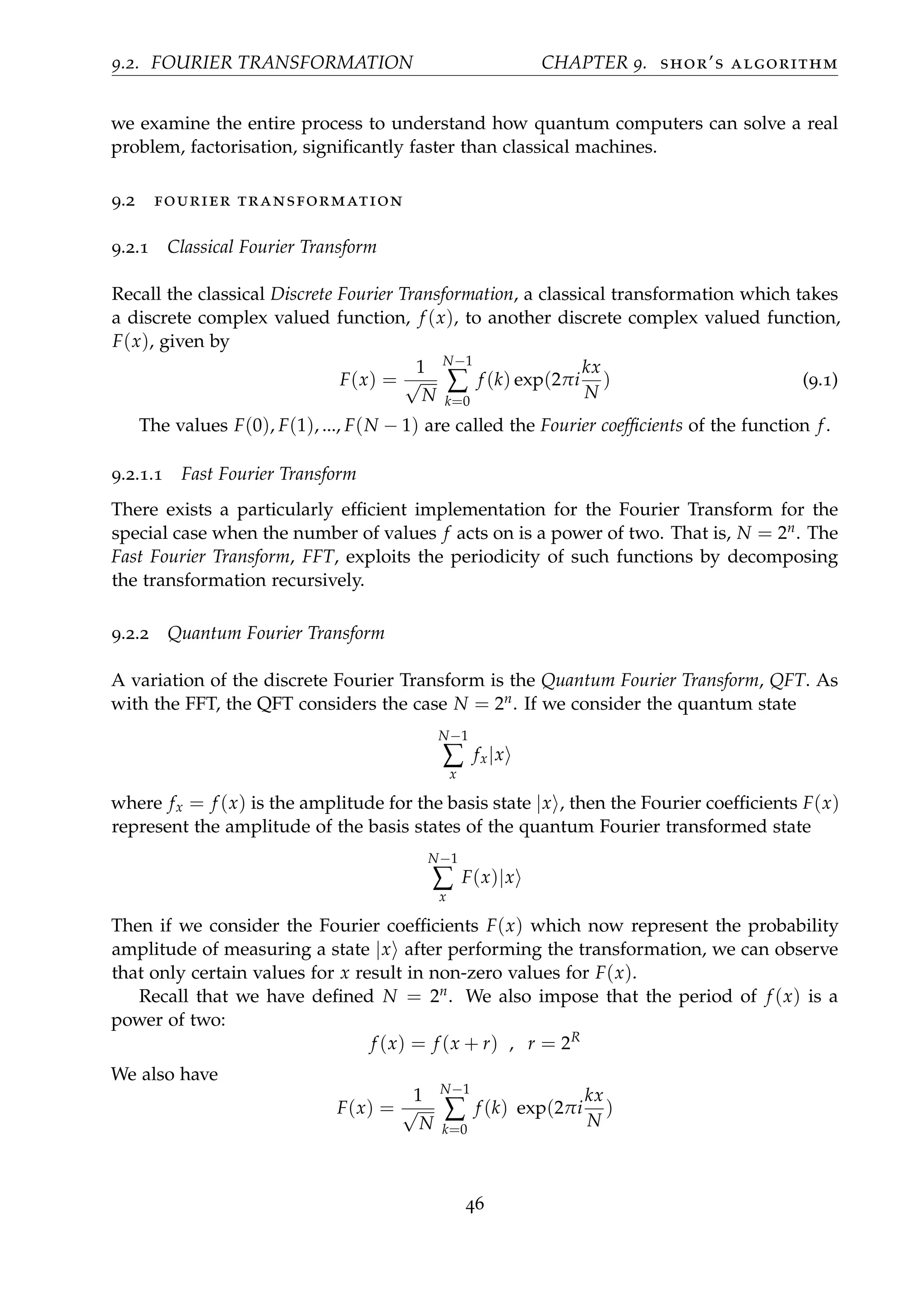
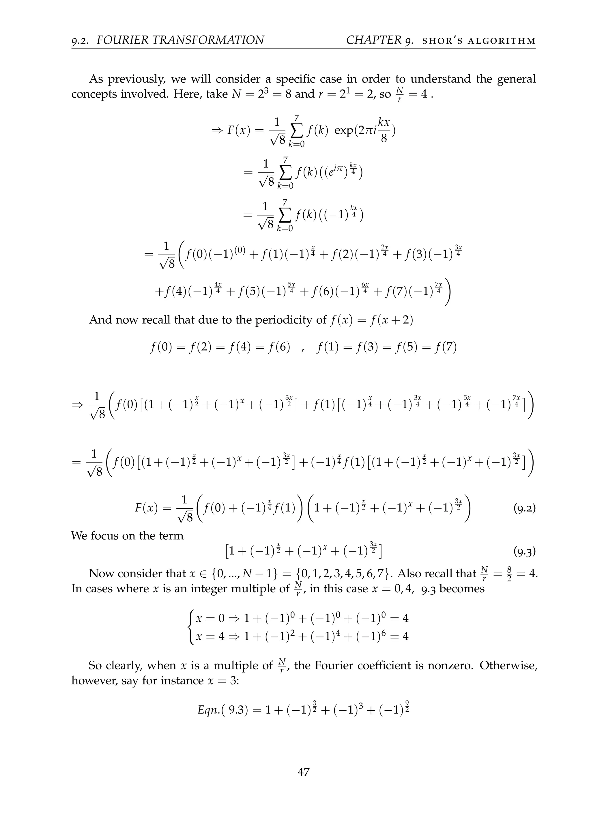
![9.3. FACTORISATION BY PERIOD FINDING CHAPTER 9. shor’s algorithm
= 1 + (−1)(−1)
1
2 + (−1) + (−1)4
(−1)
1
2
= 1 − i − 1 + i = 0
Any other value of x that isn’t an integer multiple of N
r will demonstrate this behaviour
and sum to zero. This behaviour extends to larger values of n and R such that we can
say that the only Fourier coefficients which are non zero are F(x = k N
r ), k ∈ N. In this
case, the state after QFT is a superposition of |0 and |4 :
F(0)|0 + F(1)|4 = F(0) 0(
N
r
) + F(1) 1(
N
r
)
Now that we know that the only nonzero Fourier coefficients correspond to x being
a multiple of N
r we can say that the state after Fourier transformation
F(x)|x
can only be measured to exist for such values of x. So then, if measured, the observed
value would be some k N
r . The state after performing the QFT is given by
QFT(f (x)) =
r−1
∑
k=0
F(k) k(
N
r
) (9.4)
Producing this state is the most important quantum subroutine used in quantum
computation, and we will see its use in Shor’s Algorithm. The realisation of the QFT is
explained in §7.8 of [11], which builds on the earlier idea of defining relatively simple
gates and combining them recursively.
9.3 factorisation by period finding
Recall our overall aim here: we wish to factor an integer, M, into its prime factors, mi.
For example, M = 21 = m1 × m2 = 7 × 3. Using modular addition, we define any
integer as a mod M, e.g to define 30, we say 30mod21 ≡ 9mod21. We define the order of
such an integer as the first r which satisfies
ar
− 1 ≡ 0mod M (9.5)
Example 9.1. If we consider M = 7 and we wish to find the order of a = 2, we are
considering integers
a mod M ≡ 2mod 7, 9mod 7, 16 mod 7, ...
. We have
p mod 7 ≡ 0 for p = 7, 14, 21, 28, ...
So we are looking for the lowest value of r for each a to give ar − 1 = 7k where k ∈ N.
48](https://image.slidesharecdn.com/b93d7c4e-484e-4e7c-9a0b-90813b0817a5-160722100840/75/Mathematical_Introduction_to_Quantum_Computation-53-2048.jpg)
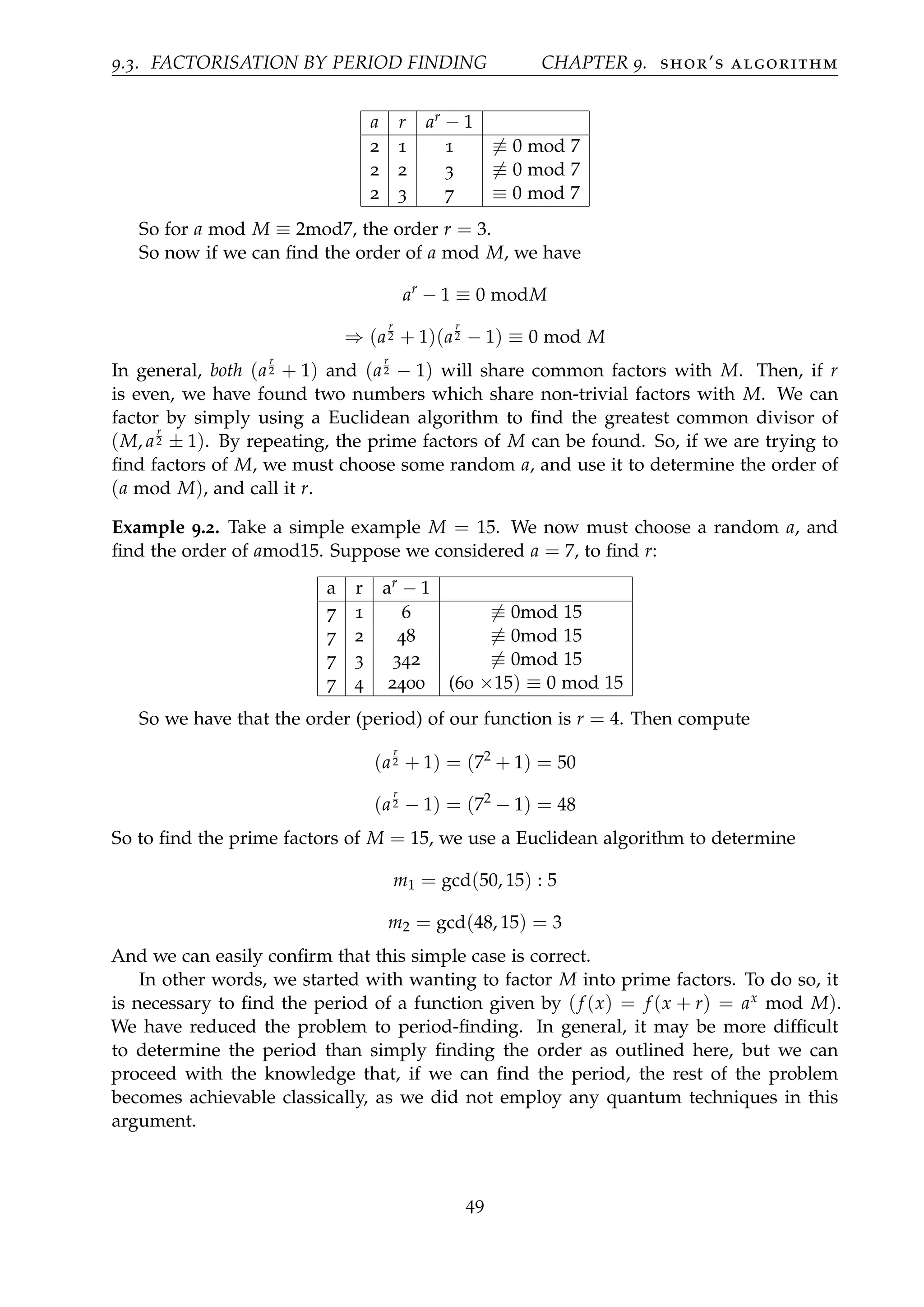
![9.4. STEPS OF SHOR’S ALGORITHM CHAPTER 9. shor’s algorithm
9.4 steps of shor’s algorithm
We are now in a position to describe the steps taken in Shor’s Algorithm to factor an
integer M into its prime factors. A preliminary to the algorithms is deciding how many
qubits to compose the system of. It can be shown (§8.3, [11]) that the number of qubits,
n, should be chosen to satisfy
M2
≤ 2n
≤ 2M2
(9.6)
We will do so a number of times. First, we will go through each step in explicit detail
and explain the concepts involved. Then, we will succinctly summarise the steps. Finally,
we will walk through the programme precisely for a specific value to be factorised.
9.4.1 Detailed Description of Steps
1. Randomly choose a value for a that is relatively prime to M. (If they are not
relatively prime then a is a factor and the rest of the algorithm is redundant, so it
is necessary to check this condition early by a simple Euclidean algorithm).
2. Since we are interested in the function f (x) = ax mod M, we generate it within the
superposition of an n-qubit state obtained through quantum parallelisation (recall
§ 8.2), by passing a register of qubits |x together with a register of |0 ’s through a
parallelisation scheme, giving the output
1
√
2n
2n−1
∑
x=0
|x |f (x) =
1
√
2n
2n−1
∑
x=0
|x |ax
modM (9.7)
Since our function is periodic in r, f (x) = f (x + r), we saw in 8.2.2 that measuring
only the second register would place the first register into a superposition over
some x0 and x0 + l.r, l ∈ Z, where the second register was observed in |f (x0) . We
introduce a function, g(x), to determine whether each x is separated from x0 by
the period or not:
g(x) =
1 f (x) = f (x0) , (x = x0 + l.r)
0 f (x) = f (x0) , (x = x0 + l.r)
After measurement of the second qubit, our system is in the state
C ∑
x
g(x) |x |f (x0) (9.8)
Where C is a scaling factor.
3. Since the two registers are not entangled, we can safely ignore the register that
holds f (x), and focus solely on the state
C ∑
x
g(x) |x (9.9)
50](https://image.slidesharecdn.com/b93d7c4e-484e-4e7c-9a0b-90813b0817a5-160722100840/75/Mathematical_Introduction_to_Quantum_Computation-55-2048.jpg)
![9.4. STEPS OF SHOR’S ALGORITHM CHAPTER 9. shor’s algorithm
Applying the Quantum Fourier Transform, 9.4:
QFT C ∑
x
g(x)|x = C2
r−1
∑
k=0
G(k) k(
N
r
) (9.10)
Where C2 is another scaling constant. g(x) has the same period, r, as f (x) and G(x)
is the Fourier coefficient for g(x), given by 9.1.
4. The above assumes that N = 2n and r = 2R. In the case that r = 2R, the transform
approximates the exact case: most of the amplitude is associated with integers
equal to or near a multiple of the ratio N
r . In this way, following this procedure,
were we to measure the system, with high probability we can say that the observed
value for x is a multiple of N
r , or else a value very near to it. Assign the measure-
ment found in this step the label β.
5. Having obtained a β, use the purely classical procedure of continued fractions to
deduce the period r. We have obtained a measurement from step 4 which we are
confident generates an integer near to a multiple of N
r , (given by β = jN
r + ε, where
ε is small compared with N). We are interested in finding r. We know N = 2n, so
if we consider the fraction
β
N
= j
N
r
1
N
+
ε
N
=
j
r
+
ε
N
In the simplest case, r = 2R, so ε = 0, and this means that simply reducing the
fraction
β
N yields a fraction which we can see as being
j
r , and we can read the
denominator as the period r we’re interested in. In general, this is not the case,
so we must consider ε = 0. In this case we apply the method of continuously
expanding fractions. This is a purely classical mathematical argument, examined
well by much of the literature on this topic, for instance in [16].
β
N
=
j
r
+
ε
N
By fraction expansion, we may continuously change the fraction
β
N to reflect a
significant fraction,
j
r with some small correction, ε
N . We aim to calculate the signif-
icant fraction and use it to read the denominator as the period r. We require that
r < M, so we terminate the procedure when the denominator of our ”significant”
fraction exceeds M.
A general fraction expansion is given by
A
B
= a0 +
1
a1 + 1
a2+ 1
...+ 1
ap
(9.11)
51](https://image.slidesharecdn.com/b93d7c4e-484e-4e7c-9a0b-90813b0817a5-160722100840/75/Mathematical_Introduction_to_Quantum_Computation-56-2048.jpg)
![9.4. STEPS OF SHOR’S ALGORITHM CHAPTER 9. shor’s algorithm
This is represented by A
B = [a0; a1, a2, ..., ap]. The the qth convergent is an approxima-
tion for A
B given by [a0, a1, ..., aq] for any 0 ≤ q ≤ p. For instance,
85
70
= [1; 4, 1, 2] = 1 +
1
4 + 1
1+ 1
1+ 1
2
= 1.214286
And if we take q1 corresponding to approximation using only one fraction, q1 =
[1; 4], we would find
83
70
≈ q1 = [1; 4] = 1 +
1
4
=
5
4
=
q1,num
q1,den
Which is a fair approximation.
⇒
85
70
= 1.214286 =
5
4
− 0.035714
If we consider q2 = [1; 4, 1]
q2 = 1 +
1
4 + 1
1
= 1 +
1
5
=
6
5
= 1.2
⇒ 1.214286 =
6
5
+ 0.014286
So we can see that every time we boil the fraction down to the next value of q, the
dominant fraction gets closer to the actual value and the correction becomes very
small.
We are trying to generate a guess for our period r, but r < M, so we are only
interested in denominators of qi which are less than M. If we say qi =
qi,num
qi,den
, we
look for the first such qi,den to satisfy (qi,den < M < qi+1,den), and we try to complete
the algorithm using r = qi,den.
Now, if we apply this to our situation: we have measured a β which we know to
be near a multiple of N
r . Take an explicit example, say N = 512 = 210, and that we
are trying to factor M = 21. Suppose the output of the quantum implementation
is β = 89.
β
N
=
89
512
= 0.173823 = [0; 5, 1, 3, 22]
= 0 +
1
5 + 1
1+ 1
3+ 1
22
We calculate the values for qi
q0 = [0] = 0
52](https://image.slidesharecdn.com/b93d7c4e-484e-4e7c-9a0b-90813b0817a5-160722100840/75/Mathematical_Introduction_to_Quantum_Computation-57-2048.jpg)
![9.4. STEPS OF SHOR’S ALGORITHM CHAPTER 9. shor’s algorithm
q1 = [0; 5] = 0 +
1
5
= 0.2
q2 = [0; 5, 1] = 0 +
1
5 + 1
1
=
1
6
= 0.16667
q3 = [0; 5, 1, 3] = 0 +
1
5 + 1
1+1
3
=
1
5 + 4
3
=
1
23
4
=
4
23
= 0.173913
q4 = [0; 5, 1, 3, 22] = 0 +
1
5 + 1
1+ 1
3+ 1
22
=
89
512
= 0.173823
Clearly, the highest qi,den < M is
(q2,den = 6) < (M = 21) < (23 = q3,den)
Thus we take r = 6 as our period and try to complete the algorithm using this.
One way to think of this is as
β =
j
r
+
ε
N
= α
j
r
In our particular example, r = 6 and
β = 89 = 1(
512
6
) + 3.67
so j = 1.
β
N
=
89
512
= 0.173828 = α0
1
6
⇒ α0 = 1.042969
After the first expanded fraction we said that q1 = [0; 5]
⇒
89
512
= 0 +
1
5
= 0.2 = α1
j
r
= α1
1
6
⇒ α1 = 1.2
Taking q2 = [0; 5, 1]
89
512
= 0 +
1
5 + 1
1
=
1
6
= α2
1
6
⇒ α2 = 1
Note this is the case we’re looking for; we’ve boiled
β
N down to
j
r . We now need to
know when we’ve gotten to this point in general.
q3 = [0; 5, 1, 3] = 0 +
1
5 + 1
1+1
3
=
4
23
= α3
1
6
⇒ α3 =
24
23
At the point where the denominator of qi exceeds M, we must have passed the case
where the denominator was the period r, since r < M, so we can read r from the
denominator of qi.
6. When r is odd, return to the start of the procedure using a different value for a.
7. When r is even, use a Euclidean algorithm to determine whether either of (a
r
2 + 1)
or (a
r
2 − 1) share a non-trivial factor with M. If so, we have found a factor of M.
53](https://image.slidesharecdn.com/b93d7c4e-484e-4e7c-9a0b-90813b0817a5-160722100840/75/Mathematical_Introduction_to_Quantum_Computation-58-2048.jpg)

![9.4. STEPS OF SHOR’S ALGORITHM CHAPTER 9. shor’s algorithm
with
g(x) =
1 x = x0 + l.r
0 x = x0 + l.r
We can now ignore the second register and focus only on the superposition
C
2047
∑
x=0
g(x)|x
3. Perform the quantum Fourier Transformation, yielding
QFT(C
2047
∑
x=0
g(x)|x ) = C2
r−1
∑
k=0
G(k)|k
4. Measure the system after this transformation. This will result in some β. Suppose
we measure β = 206.
5. Compute
β
N
=
206
2048
=
103
1024
By continued fraction expansion this can be represented by
103
1024
= 0 +
1
9 + 1
1+ 1
16+ 1
6
We calculate the values of q for this fraction
q0 = [0] = 0
q1 = [0; 9] =
1
9
q2 = [0; 9, 1] =
1
10
q3 = [0; 9, 1, 16] =
17
169
q4 = [0; 9, 1, 16, 6] =
103
1024
Considering the denominators of these shows that q2,den < M < q3,den holds:
10 < 35 < 169
So we proceed using r = q2,den = 10.
6. r is not odd, so we move to the next step.
55](https://image.slidesharecdn.com/b93d7c4e-484e-4e7c-9a0b-90813b0817a5-160722100840/75/Mathematical_Introduction_to_Quantum_Computation-60-2048.jpg)
![9.5. EFFICIENCY IMPROVEMENT CHAPTER 9. shor’s algorithm
7. r is even, so we compute (a
r
2 ± 1)
(6
10
2 + 1) = (65
+ 1) = 7777
(6
10
2 − 1) = (65
− 1) = 7775
Then use the Euclidean algorithm to show that
m1 = gcd(7777, 35) = 7
m2 = gcd(7775, 35) = 5
Thus we have found 35 = m1.m2 = 7 × 5, and we can verify that, for this simple
case, the algorithm works.
It is worth noting here that the period of (f (x) = 6x mod 35) is in fact 2:
62
mod 35 ≡ 1
64
mod 35 ≡ 1
...
610
mod 35 ≡ 1
Yet the algorithm still worked and found the correct factorisation for 35.
9.5 efficiency improvement
In order that we can understand the improvement offered by Shor’s factoring algo-
rithm, we must consider how many steps it requires for its implementation, and
compare this with the number of steps a classical algorithm would take
9.5.1 Classical Factorisation
The general approach, [14], to finding a factor of M is to sequentially compute
M
1
,
M
2
,
M
3
, ... ,
M
√
M
In some cases, a suitable factor will appear very early in this procedure, but in
some cases it could take all
√
M attempts. On average, it is fair to say that it will
take
√
M
2 trials to identify a factor. Each iteration will have some time expense, we
will say as small as 10−12 seconds, so let us consider how many trials a realistic
problem would require and find how long it would take a classical computer to
solve this.
56](https://image.slidesharecdn.com/b93d7c4e-484e-4e7c-9a0b-90813b0817a5-160722100840/75/Mathematical_Introduction_to_Quantum_Computation-61-2048.jpg)
![9.5. EFFICIENCY IMPROVEMENT CHAPTER 9. shor’s algorithm
Example 9.3. If the number we wish to factorise, M, has, for instance, 77 digits, we
can sat that is of the order 2256 since 2256 = 1.15 × 1077. Then
√
M ∼ (2256
)
1
2 = 2128
⇒
√
M
2
∼ (2128
)−1
= 2127
Trials
In time, this will take
2127
Trials × 10−12
seconds per Trial
∼ 1026
seconds
The universe is approximately 4 × 10¹⁷ seconds old, so obviously trying to factor
such a number is not achievable classically. The best known factoring algorithm,
the number field sieve, [17] offers an improvement over this time scale, but not by
nearly the same amount as the improvement offered by quantum computing, [18].
9.5.2 Quantum Factoring Algorithm
The most demanding part of the algorithm is the modular exponentiation required to
generate the calculation of f (x) = ax mod M inside the state. §6.4 of [11] discusses
this generation in detail, and Shor shows that it can be most efficiently achieved in
O(n2 log2 n log2 log2 n) time steps, where n is the number of qubits involved in
the system [19]. (Recall N = 2n)
Rieffel and Polak also discuss the number of steps required of each section of
the algorithm as outlined here, §8.4 of [11]. Clearly the most computationally
expensive calculation is that of modular exponentiation, which we have seen to
cost of the order (n2 log2 n log2 log2 n) in time.
Again aiming to factorise a number of the order 2256, we must first find what size
of a system (number of qubits) would be required. This is determined by
M2
≤ 2n
≤ 2M2
⇒ 2512
≤ 2n
≤ 2513
In general M will not be a power of two, and there will be only one such n to satisfy
this condition. It suffices here to choose n = 512. The majority of the computation
is due to the modular exponentiation, so we must calculate O(n2 log2 nlog2log2 n)
to get an idea of how many steps are needed.
n = 512 ⇒ log2n = log2(29
)
⇒ log2 n = 9
57](https://image.slidesharecdn.com/b93d7c4e-484e-4e7c-9a0b-90813b0817a5-160722100840/75/Mathematical_Introduction_to_Quantum_Computation-62-2048.jpg)
![9.5. EFFICIENCY IMPROVEMENT CHAPTER 9. shor’s algorithm
⇒ log2 log2 n = log2(9) ≈ 3
⇒ n2
log2 n log2 log2 n = (512)2
× 9 × 3
= 7, 077, 888 Trials
⇒ Time = (7, 077, 888 Trials) × (10−12
seconds per Trial)
= 7 × 10⁻⁶
seconds
This is clear evidence that Shor’s Algorithm is definitively faster than any classical
algorithm can ever achieve.
Thus, we have given a concrete example of a case where quantum computing can
be implemented to solve a real problem which cannot be efficiently dealt with
by a classical computer. There are, however, many other promising applications,
such as the needle-in-the-haystack problem addressed by Grover’s Algorithm, [20].
There is potential to model quantum chemistry far more accurately than is done at
present by modelling chemical bonds at quantum levels through use of quantum
computation, [21]. Such modelling currently occupies a huge amount of computa-
tional resources worldwide in trying to achieve accurate models at quantum scales.
It is thought that quantum computers may be able to save resources and help in
the modelling of specific chemical bonds at quantum levels, [22], and therefore
help in the development of more effective medicines. These are only some of the
vast possible applications of the technology, and so it is clear that there is suffi-
cient motivation for the field to develop and to potentially shape the technological
landscape over the coming years and decades.
58](https://image.slidesharecdn.com/b93d7c4e-484e-4e7c-9a0b-90813b0817a5-160722100840/75/Mathematical_Introduction_to_Quantum_Computation-63-2048.jpg)
![B I B L I O G R A P H Y
[1] Yu I Manin. Vychislimoe i nevychislimoe (computable and noncomputable),
moscow: Sov, 1980.
[2] Richard P Feynman. Simulating physics with computers. International journal of
theoretical physics, 21(6):467–488, 1982.
[3] Paul Benioff. Quantum mechanical hamiltonian models of turing machines. Journal
of Statistical Physics, 29(3):515–546, 1982.
[4] David Deutsch. Quantum theory, the church-turing principle and the universal
quantum computer. In Proceedings of the Royal Society of London A: Mathematical,
Physical and Engineering Sciences, volume 400, pages 97–117. The Royal Society, 1985.
[5] David Deutsch and Richard Jozsa. Rapid solution of problems by quantum compu-
tation. Proceedings of the Royal Society of London. Series A: Mathematical and Physical
Sciences, 439(1907):553–558, 1992.
[6] Peter W Shor. Algorithms for quantum computation: Discrete logarithms and fac-
toring. In Foundations of Computer Science, 1994 Proceedings., 35th Annual Symposium
on, pages 124–134. IEEE, 1994.
[7] Michael A Nielsen and Isaac L Chuang. Quantum computation and quantum informa-
tion. Cambridge university press, 2010.
[8] Charles H Bennett, Gilles Brassard, Claude Cr´epeau, Richard Jozsa, Asher Peres,
and William K Wootters. Teleporting an unknown quantum state via dual classical
and einstein-podolsky-rosen channels. Physical review letters, 70(13):1895, 1993.
[9] WK Wooters and WK Zurek. Quantum no-cloning theorem. Nature, 299:802, 1982.
[10] Mark M Wilde. Quantum information theory. Cambridge University Press, 2013.
[11] Eleanor G Rieffel and Wolfgang H Polak. Quantum computing: A gentle introduction.
MIT Press, 2011.
[12] Bernard J. Fino and V. Ralph Algazi. Unified matrix treatment of the fast walsh-
hadamard transform. IEEE Transactions on Computers, 25(11):1142–1146, 1976.
[13] Daniel R Simon. On the power of quantum computation. SIAM journal on computing,
26(5):1474–1483, 1997.
[14] John M Pollard. A monte carlo method for factorization. BIT Numerical Mathematics,
15(3):331–334, 1975.
[15] Isaac Chuang, Raymond Laflamme, P Shor, and W Zurek. Quantum computers,
factoring, and decoherence. arXiv preprint quant-ph/9503007, 1995.
[16] C Lavor, LRU Manssur, and R Portugal. Shor’s algorithm for factoring large integers.
arXiv preprint quant-ph/0303175, 2003.
60](https://image.slidesharecdn.com/b93d7c4e-484e-4e7c-9a0b-90813b0817a5-160722100840/75/Mathematical_Introduction_to_Quantum_Computation-65-2048.jpg)
![BIBLIOGRAPHY BIBLIOGRAPHY
[17] Arjen K Lenstra, Hendrik W Lenstra Jr, Mark S Manasse, and John M Pollard. The
number field sieve. Springer, 1993.
[18] Shah Muhammad Hamdi, Syed Tauhid Zuhori, Firoz Mahmud, and Biprodip Pal.
A compare between shor’s quantum factoring algorithm and general number field
sieve. In Electrical Engineering and Information & Communication Technology (ICEEICT),
2014 International Conference on, pages 1–6. IEEE, 2014.
[19] Peter W Shor. Polynomial-time algorithms for prime factorization and discrete log-
arithms on a quantum computer. SIAM journal on computing, 26(5):1484–1509, 1997.
[20] Lov K Grover. A fast quantum mechanical algorithm for database search. In Pro-
ceedings of the twenty-eighth annual ACM symposium on Theory of computing, pages
212–219. ACM, 1996.
[21] Benjamin P Lanyon, James D Whitfield, GG Gillett, Michael E Goggin, Marcelo P
Almeida, Ivan Kassal, Jacob D Biamonte, Masoud Mohseni, Ben J Powell, Marco Bar-
bieri, et al. Towards quantum chemistry on a quantum computer. Nature Chemistry,
2(2):106–111, 2010.
[22] Christof Zalka. Simulating quantum systems on a quantum computer. Proceedings
of the Royal Society of London. Series A: Mathematical, Physical and Engineering Sciences,
454(1969):313–322, 1998.
61](https://image.slidesharecdn.com/b93d7c4e-484e-4e7c-9a0b-90813b0817a5-160722100840/75/Mathematical_Introduction_to_Quantum_Computation-66-2048.jpg)


