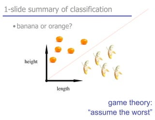
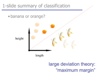
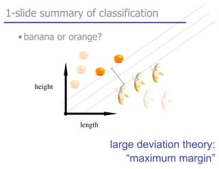
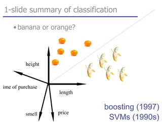
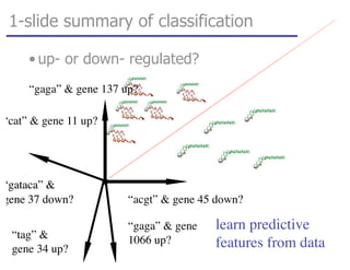
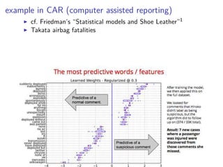
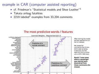
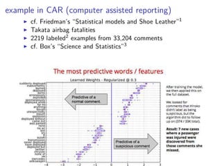
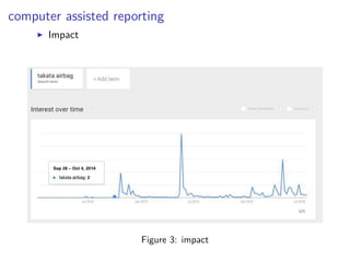
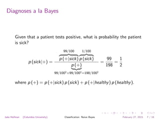
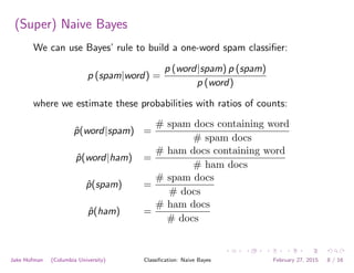
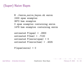
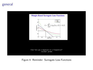
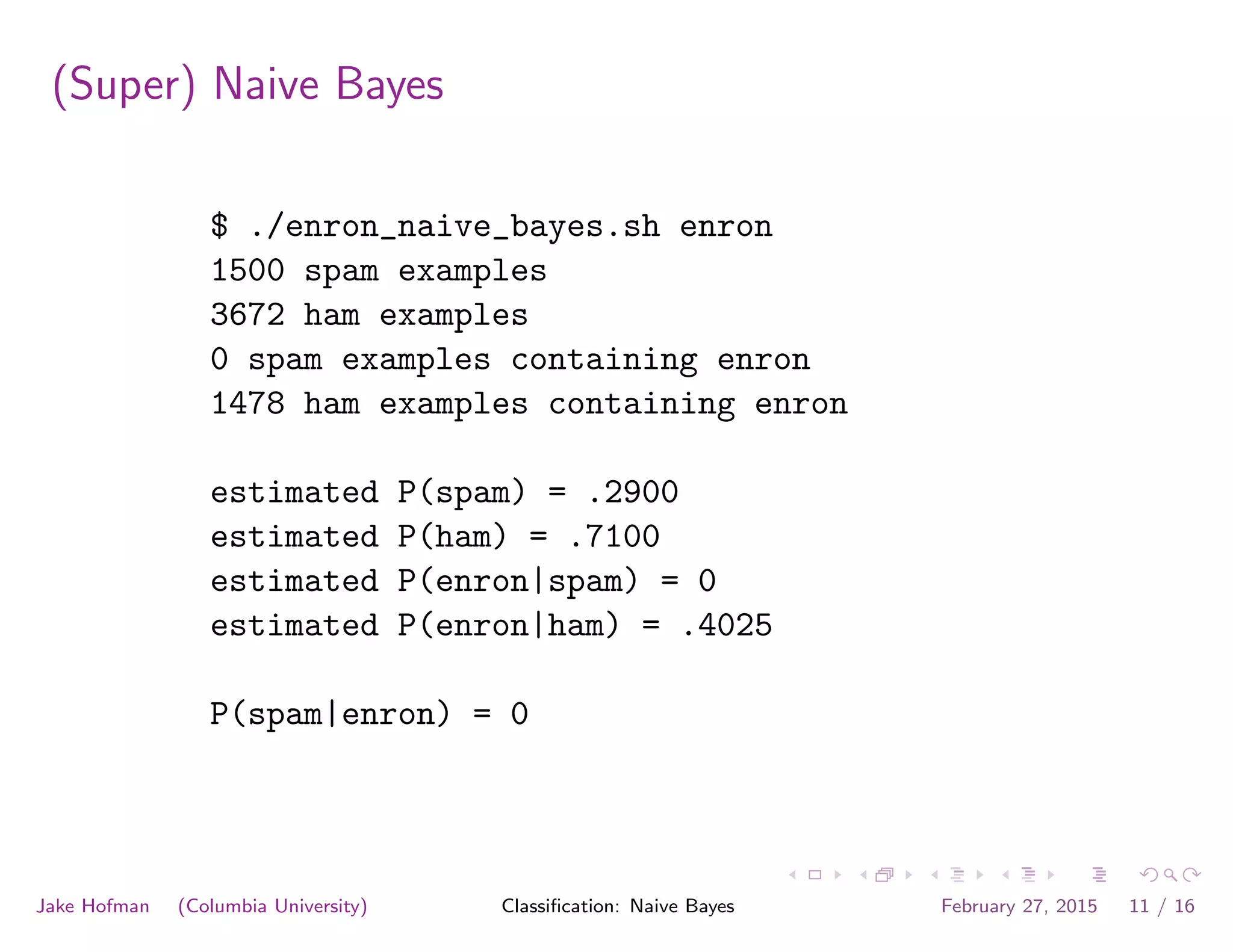
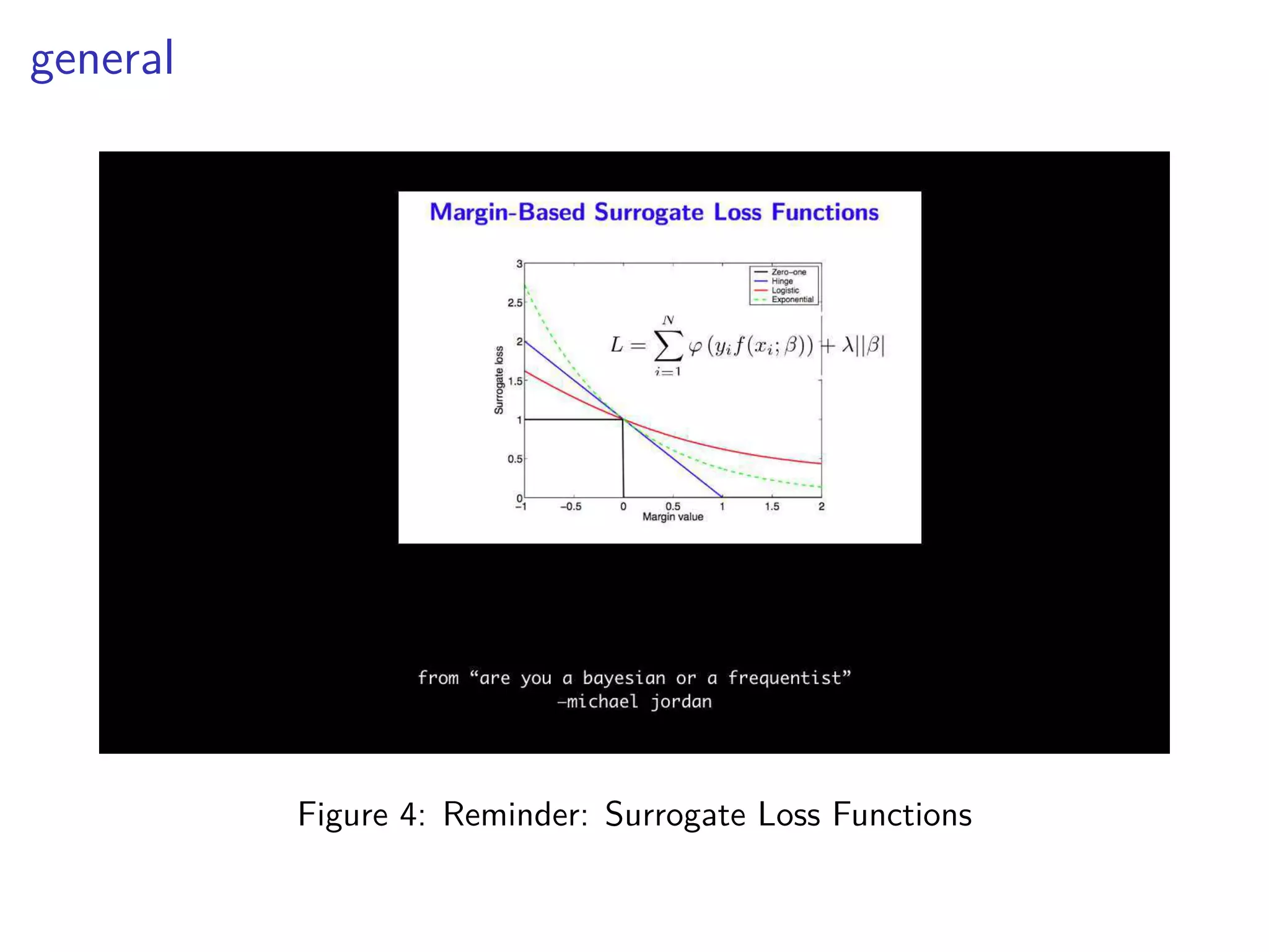
This document discusses various machine learning classification techniques, including naive Bayes classification and boosting. It provides mathematical explanations and code examples for naive Bayes classification using word counts from documents. It also summarizes boosting as minimizing a convex surrogate loss function by iteratively adding weak learners to improve predictive performance. Examples are given of using an exponential loss function and calculating weight updates in boosting.


![tangent: logistic function as surrogate loss function
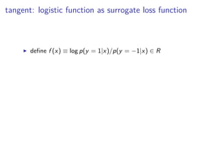
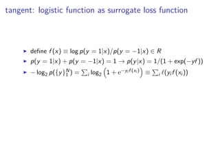
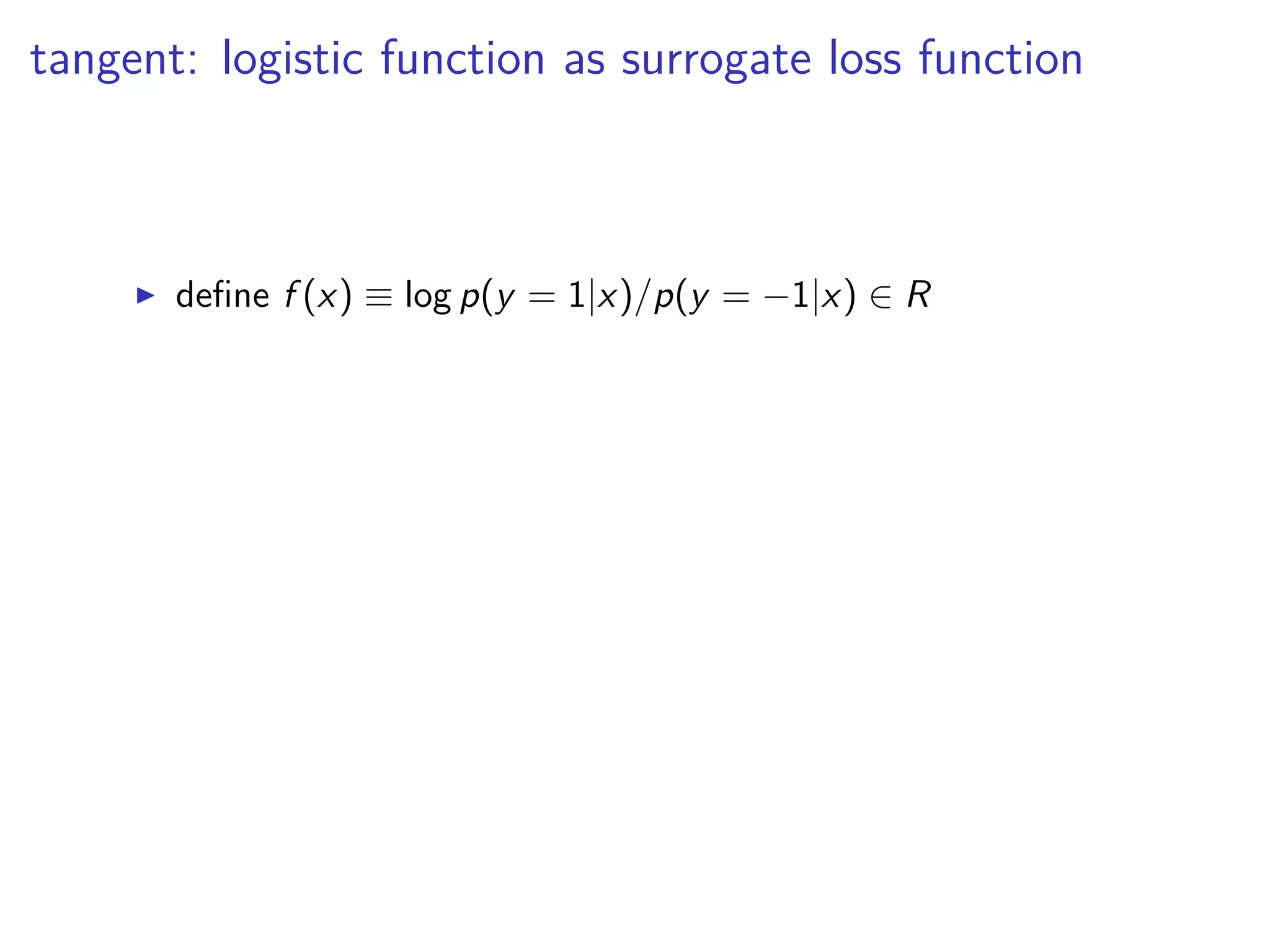
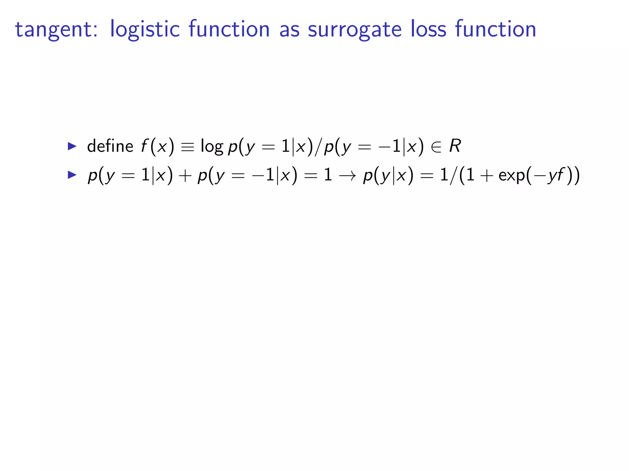
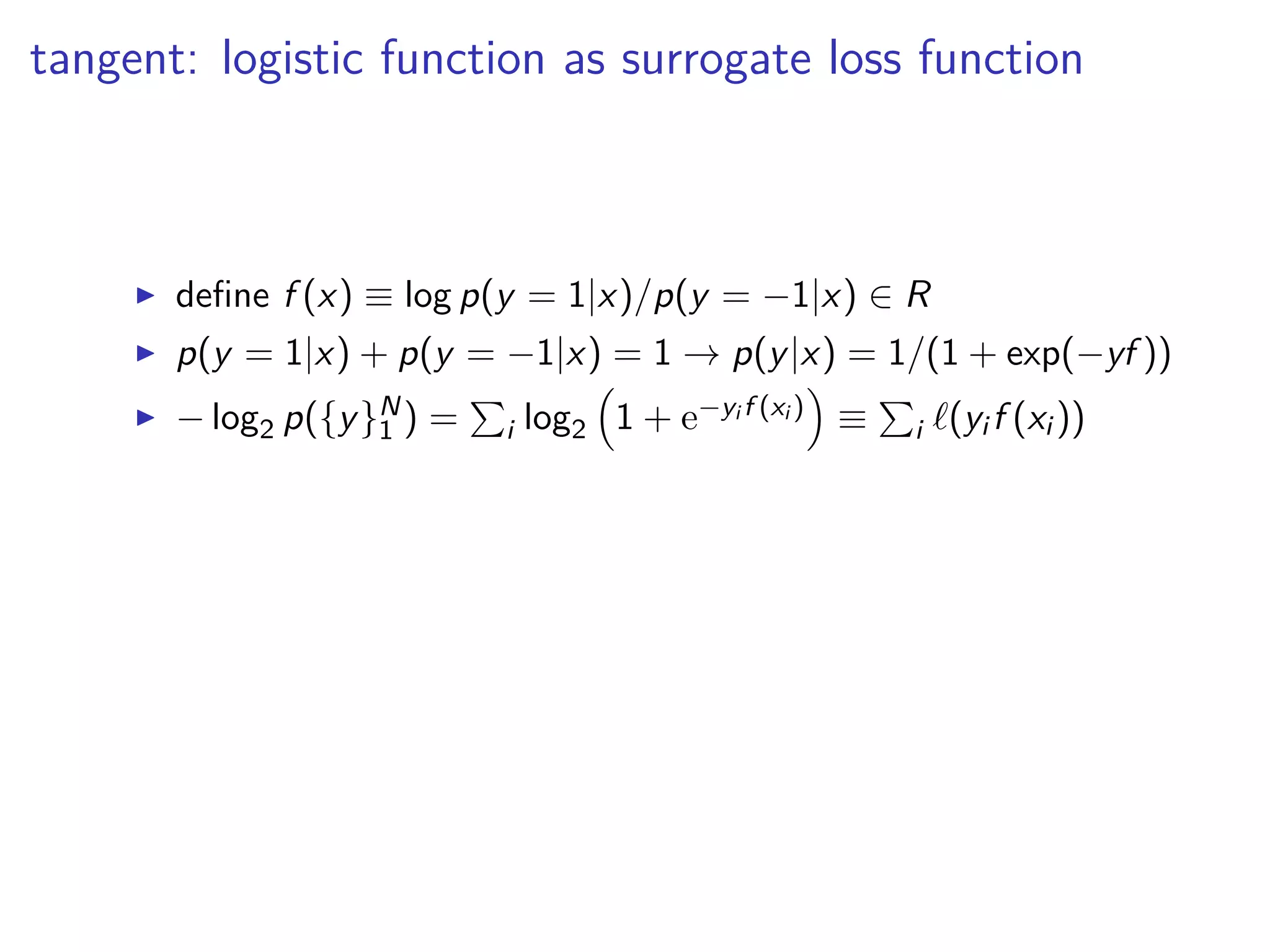
◮ define f (x) ≡ log p(y = 1|x)/p(y = −1|x) ∈ R
◮ p(y = 1|x) + p(y = −1|x) = 1 → p(y|x) = 1/(1 + exp(−yf ))
◮ − log2 p({y}N
1 ) = i log2 1 + e−yi f (xi ) ≡ i ℓ(yi f (xi ))
◮ ℓ′′ > 0, ℓ(µ) > 1[µ < 0] ∀µ ∈ R.](https://image.slidesharecdn.com/lecture8-170405174424/85/Modeling-Social-Data-Lecture-8-Classification-47-320.jpg)
![tangent: logistic function as surrogate loss function
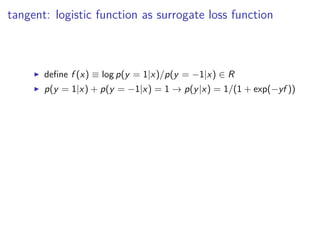
◮ define f (x) ≡ log p(y = 1|x)/p(y = −1|x) ∈ R
◮ p(y = 1|x) + p(y = −1|x) = 1 → p(y|x) = 1/(1 + exp(−yf ))
◮ − log2 p({y}N
1 ) = i log2 1 + e−yi f (xi ) ≡ i ℓ(yi f (xi ))
◮ ℓ′′ > 0, ℓ(µ) > 1[µ < 0] ∀µ ∈ R.
◮ ∴ maximizing log-likelihood is minimizing a surrogate convex
loss function for classification](https://image.slidesharecdn.com/lecture8-170405174424/85/Modeling-Social-Data-Lecture-8-Classification-48-320.jpg)
![tangent: logistic function as surrogate loss function
◮ define f (x) ≡ log p(y = 1|x)/p(y = −1|x) ∈ R
◮ p(y = 1|x) + p(y = −1|x) = 1 → p(y|x) = 1/(1 + exp(−yf ))
◮ − log2 p({y}N
1 ) = i log2 1 + e−yi f (xi ) ≡ i ℓ(yi f (xi ))
◮ ℓ′′ > 0, ℓ(µ) > 1[µ < 0] ∀µ ∈ R.
◮ ∴ maximizing log-likelihood is minimizing a surrogate convex
loss function for classification
◮ but i log2 1 + e−yi wT h(xi ) not as easy as i e−yi wT h(xi )](https://image.slidesharecdn.com/lecture8-170405174424/85/Modeling-Social-Data-Lecture-8-Classification-49-320.jpg)
![boosting 1
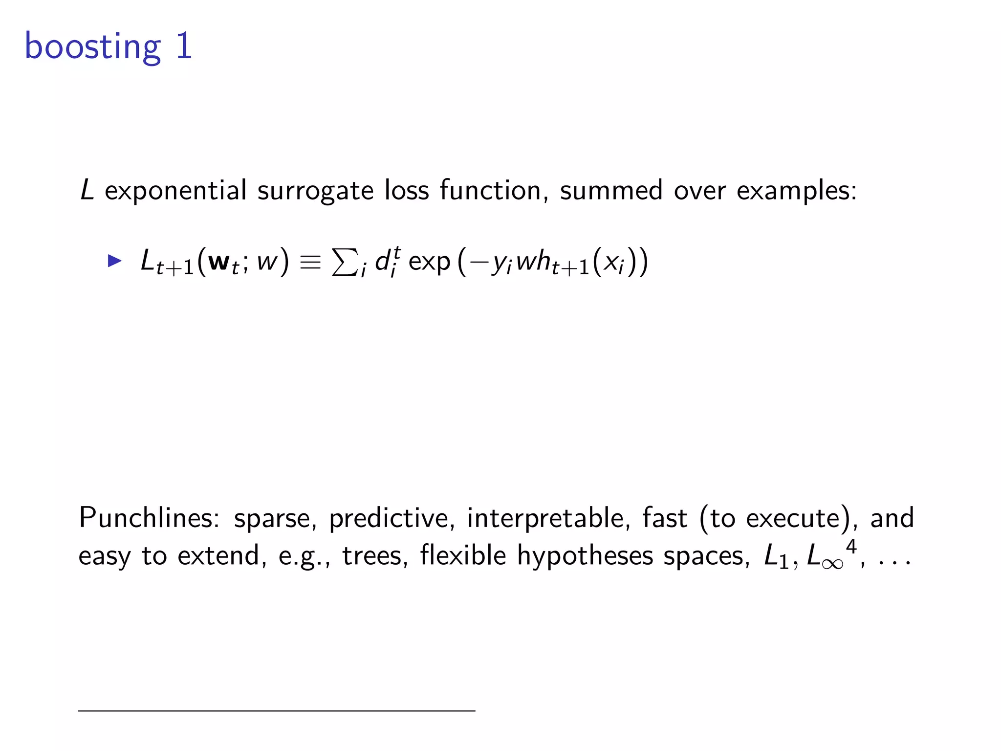
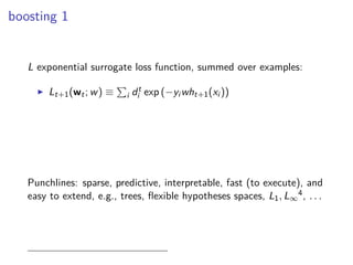
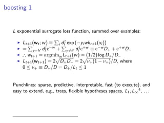
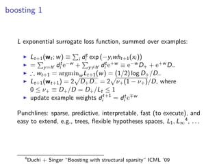
L exponential surrogate loss function, summed over examples:
◮ L[F] = i exp (−yi F(xi ))](https://image.slidesharecdn.com/lecture8-170405174424/85/Modeling-Social-Data-Lecture-8-Classification-50-320.jpg)
![boosting 1
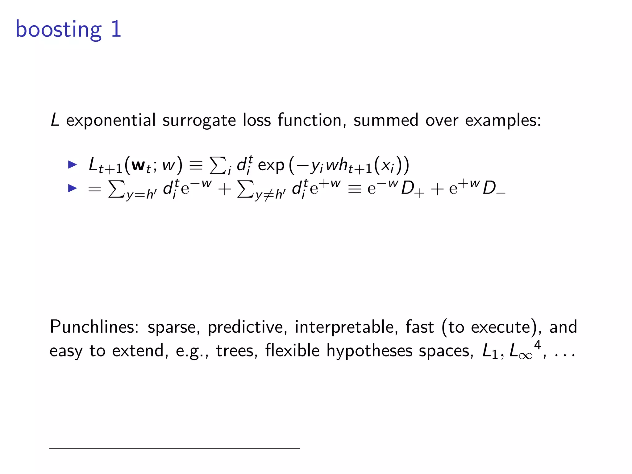
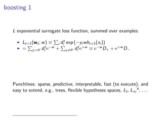
L exponential surrogate loss function, summed over examples:
◮ L[F] = i exp (−yi F(xi ))
◮ = i exp −yi
t
t′ wt′ ht′ (xi ) ≡ Lt(wt)](https://image.slidesharecdn.com/lecture8-170405174424/85/Modeling-Social-Data-Lecture-8-Classification-51-320.jpg)
![boosting 1
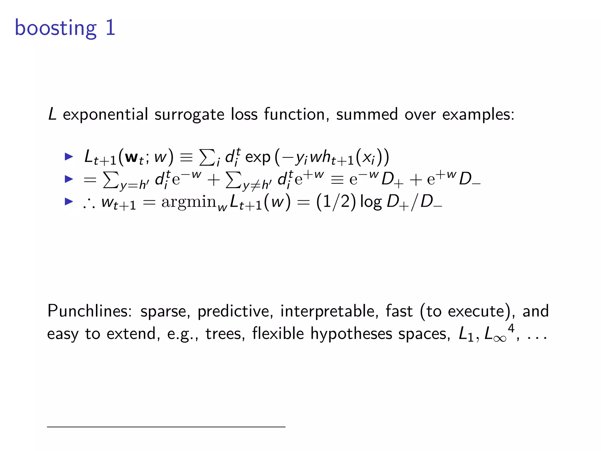
L exponential surrogate loss function, summed over examples:
◮ L[F] = i exp (−yi F(xi ))
◮ = i exp −yi
t
t′ wt′ ht′ (xi ) ≡ Lt(wt)
◮ Draw ht ∈ H large space of rules s.t. h(x) ∈ {−1, +1}](https://image.slidesharecdn.com/lecture8-170405174424/85/Modeling-Social-Data-Lecture-8-Classification-52-320.jpg)
![boosting 1
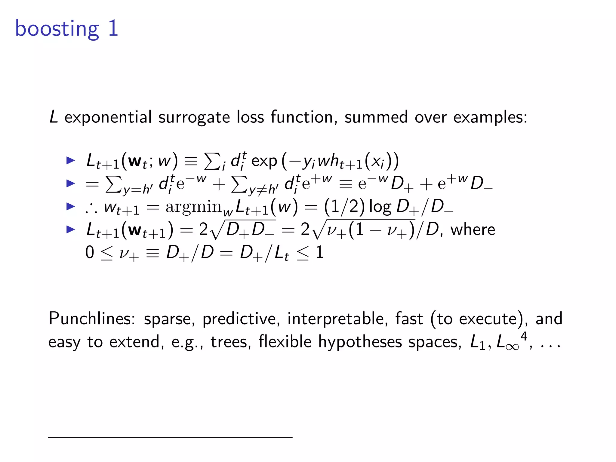
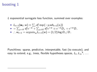
L exponential surrogate loss function, summed over examples:
◮ L[F] = i exp (−yi F(xi ))
◮ = i exp −yi
t
t′ wt′ ht′ (xi ) ≡ Lt(wt)
◮ Draw ht ∈ H large space of rules s.t. h(x) ∈ {−1, +1}
◮ label y ∈ {−1, +1}](https://image.slidesharecdn.com/lecture8-170405174424/85/Modeling-Social-Data-Lecture-8-Classification-53-320.jpg)


![tangent: logistic function as surrogate loss function
◮ define f (x) ≡ log p(y = 1|x)/p(y = −1|x) ∈ R
◮ p(y = 1|x) + p(y = −1|x) = 1 → p(y|x) = 1/(1 + exp(−yf ))
◮ − log2 p({y}N
1 ) = i log2 1 + e−yi f (xi ) ≡ i ℓ(yi f (xi ))
◮ ℓ′′ > 0, ℓ(µ) > 1[µ < 0] ∀µ ∈ R.](https://image.slidesharecdn.com/lecture8-170405174424/75/Modeling-Social-Data-Lecture-8-Classification-47-2048.jpg)
![tangent: logistic function as surrogate loss function
◮ define f (x) ≡ log p(y = 1|x)/p(y = −1|x) ∈ R
◮ p(y = 1|x) + p(y = −1|x) = 1 → p(y|x) = 1/(1 + exp(−yf ))
◮ − log2 p({y}N
1 ) = i log2 1 + e−yi f (xi ) ≡ i ℓ(yi f (xi ))
◮ ℓ′′ > 0, ℓ(µ) > 1[µ < 0] ∀µ ∈ R.
◮ ∴ maximizing log-likelihood is minimizing a surrogate convex
loss function for classification](https://image.slidesharecdn.com/lecture8-170405174424/75/Modeling-Social-Data-Lecture-8-Classification-48-2048.jpg)
![tangent: logistic function as surrogate loss function
◮ define f (x) ≡ log p(y = 1|x)/p(y = −1|x) ∈ R
◮ p(y = 1|x) + p(y = −1|x) = 1 → p(y|x) = 1/(1 + exp(−yf ))
◮ − log2 p({y}N
1 ) = i log2 1 + e−yi f (xi ) ≡ i ℓ(yi f (xi ))
◮ ℓ′′ > 0, ℓ(µ) > 1[µ < 0] ∀µ ∈ R.
◮ ∴ maximizing log-likelihood is minimizing a surrogate convex
loss function for classification
◮ but i log2 1 + e−yi wT h(xi ) not as easy as i e−yi wT h(xi )](https://image.slidesharecdn.com/lecture8-170405174424/75/Modeling-Social-Data-Lecture-8-Classification-49-2048.jpg)
![boosting 1
L exponential surrogate loss function, summed over examples:
◮ L[F] = i exp (−yi F(xi ))](https://image.slidesharecdn.com/lecture8-170405174424/75/Modeling-Social-Data-Lecture-8-Classification-50-2048.jpg)
![boosting 1
L exponential surrogate loss function, summed over examples:
◮ L[F] = i exp (−yi F(xi ))
◮ = i exp −yi
t
t′ wt′ ht′ (xi ) ≡ Lt(wt)](https://image.slidesharecdn.com/lecture8-170405174424/75/Modeling-Social-Data-Lecture-8-Classification-51-2048.jpg)
![boosting 1
L exponential surrogate loss function, summed over examples:
◮ L[F] = i exp (−yi F(xi ))
◮ = i exp −yi
t
t′ wt′ ht′ (xi ) ≡ Lt(wt)
◮ Draw ht ∈ H large space of rules s.t. h(x) ∈ {−1, +1}](https://image.slidesharecdn.com/lecture8-170405174424/75/Modeling-Social-Data-Lecture-8-Classification-52-2048.jpg)
![boosting 1
L exponential surrogate loss function, summed over examples:
◮ L[F] = i exp (−yi F(xi ))
◮ = i exp −yi
t
t′ wt′ ht′ (xi ) ≡ Lt(wt)
◮ Draw ht ∈ H large space of rules s.t. h(x) ∈ {−1, +1}
◮ label y ∈ {−1, +1}](https://image.slidesharecdn.com/lecture8-170405174424/75/Modeling-Social-Data-Lecture-8-Classification-53-2048.jpg)