optimal merge pattern notes - algorithms

OPTIMAL MERGE PATTERN
f1,f2,f3,f4,f5={23,30,10,5,30}

Method 1
• M1=merge f1 and f220+30=50
• M2=merge M1 and f350+10=60
• M3=merge M2 and f460+5=65
• M4=merge M3 and f565+30=95

Method 2
• M1=merge f4 and f35+10=15
• M2=merge M1 and f115+20=35
• M3=merge M2 and f235+30=65
• M4=merge M3 and f565+30=95
• Total=15+35+65+95=210

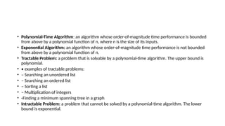
• Polynomial-Time Algorithm: an algorithm whose order-of-magnitude time performance is bounded
from above by a polynomial function of n, where n is the size of its inputs.
• Exponential Algorithm: an algorithm whose order-of-magnitude time performance is not bounded
from above by a polynomial function of n.
• Tractable Problem: a problem that is solvable by a polynomial-time algorithm. The upper bound is
polynomial.
• • examples of tractable problems:
• – Searching an unordered list
• – Searching an ordered list
• – Sorting a list
• – Multiplication of integers
• -Finding a minimum spanning tree in a graph
• Intractable Problem: a problem that cannot be solved by a polynomial-time algorithm. The lower
bound is exponential.

• examples of intractable problems (ones that have been proven to have no
polynomial-time algorithm).
∗ Towers of Hanoi: we can prove that any algorithm that solves this problem
must have a worst-case running time that is at least 2n − 1.
∗ List all permutations (all possible orderings) of n numbers. – Others have
polynomial amounts of output, but still cannot be solved in polynomial time:
∗ For an n × n draughts board with an arrangement of pieces, determine
whether there is a winning strategy for White (i.e. a sequence of moves so
that, no matter what Black does, White is guaranteed to win). We can prove
that any algorithm that solves this problem must have a worst-case running
time that is at least 2n.

NP- algorithms- NP-hardness and NP-completeness
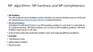
• NP Problem:
The NP problems set of problems whose solutions are hard to find but easy to verify and
are solved by Non-Deterministic Machine in polynomial time.
• NP-Hard Problem:
A Problem X is NP-Hard if there is an NP-Complete problem Y, such that Y is reducible to
X in polynomial time. NP-Hard problems are as hard as NP-Complete problems. NP-Hard
Problem need not be in NP class.
• A lot of times takes the particular problem solve and reducing different problems.
• example :
• Hamiltonian cycle .
• optimization problem .
• Shortest path

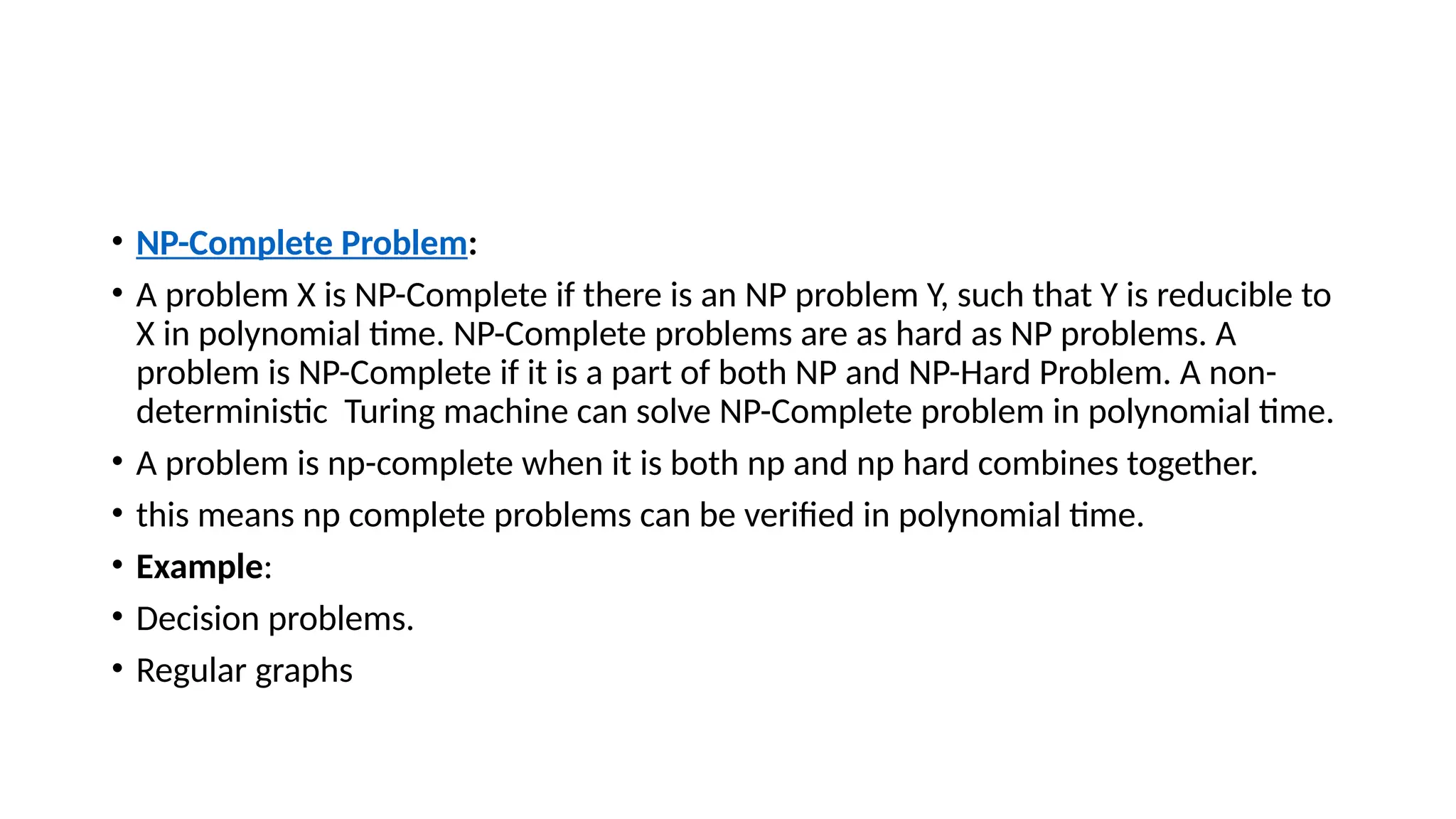
• NP-Complete Problem:
• A problem X is NP-Complete if there is an NP problem Y, such that Y is reducible to
X in polynomial time. NP-Complete problems are as hard as NP problems. A
problem is NP-Complete if it is a part of both NP and NP-Hard Problem. A non-
deterministic Turing machine can solve NP-Complete problem in polynomial time.
• A problem is np-complete when it is both np and np hard combines together.
• this means np complete problems can be verified in polynomial time.
• Example:
• Decision problems.
• Regular graphs

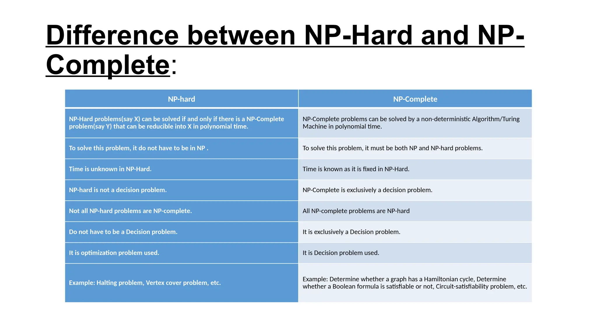
Difference between NP-Hard and NP-
Complete:
NP-hard NP-Complete
NP-Hard problems(say X) can be solved if and only if there is a NP-Complete
problem(say Y) that can be reducible into X in polynomial time.
NP-Complete problems can be solved by a non-deterministic Algorithm/Turing
Machine in polynomial time.
To solve this problem, it do not have to be in NP . To solve this problem, it must be both NP and NP-hard problems.
Time is unknown in NP-Hard. Time is known as it is fixed in NP-Hard.
NP-hard is not a decision problem. NP-Complete is exclusively a decision problem.
Not all NP-hard problems are NP-complete. All NP-complete problems are NP-hard
Do not have to be a Decision problem. It is exclusively a Decision problem.
It is optimization problem used. It is Decision problem used.
Example: Halting problem, Vertex cover problem, etc.
Example: Determine whether a graph has a Hamiltonian cycle, Determine
whether a Boolean formula is satisfiable or not, Circuit-satisfiability problem, etc.

• TSP is NP-Complete
• The traveling salesman problem consists of a salesman and a set of cities. The salesman has to
visit each one of the cities starting from a certain one and returning to the same city. The
challenge of the problem is that the traveling salesman wants to minimize the total length of
the trip
• Proof
• To prove TSP is NP-Complete, first we have to prove that TSP belongs to NP. In TSP, we find a
tour and check that the tour contains each vertex once. Then the total cost of the edges of the
tour is calculated. Finally, we check if the cost is minimum. This can be completed in polynomial
time. Thus TSP belongs to NP.
• Secondly, we have to prove that TSP is NP-hard. To prove this, one way is to show
that Hamiltonian cycle ≤p TSP (as we know that the Hamiltonian cycle problem is NPcomplete).
• Assume G = (V, E) to be an instance of Hamiltonian cycle.

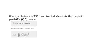
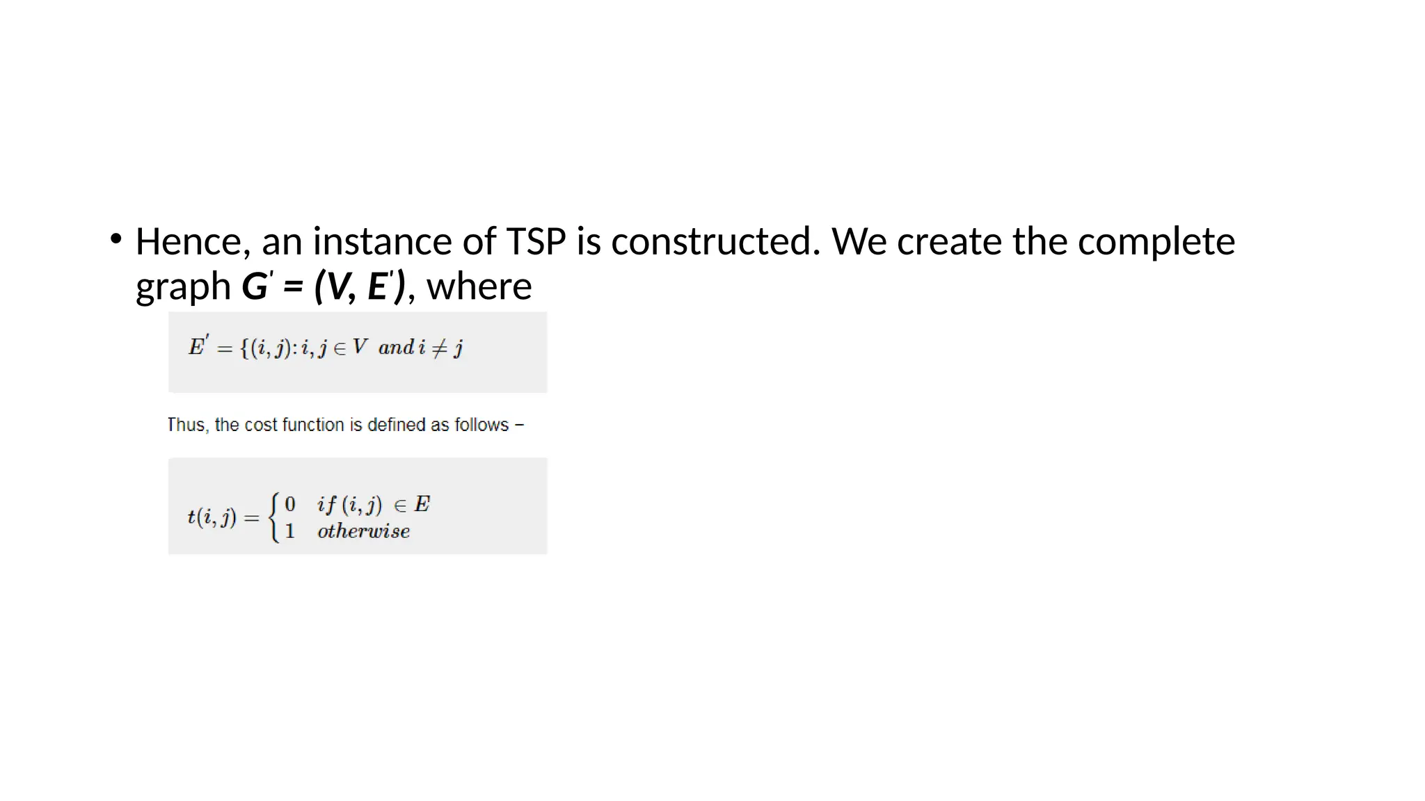
• Hence, an instance of TSP is constructed. We create the complete
graph G'
= (V, E'
), where

• Now, suppose that a Hamiltonian cycle h exists in G. It is clear that the
cost of each edge in h is 0 in G'
as each edge belongs to E.
Therefore, h has a cost of 0 in G'
. Thus, if graph G has a Hamiltonian
cycle, then graph G'
has a tour of 0 cost.
• Conversely, we assume that G'
has a tour h'
of cost at most 0. The cost
of edges in E'
are 0 and 1 by definition. Hence, each edge must have a
cost of 0 as the cost of h'
is 0. We therefore conclude that h'
contains
only edges in E.
• We have thus proven that G has a Hamiltonian cycle, if and only
if G'
has a tour of cost at most 0. TSP is NP-complete.

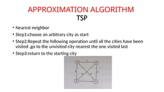
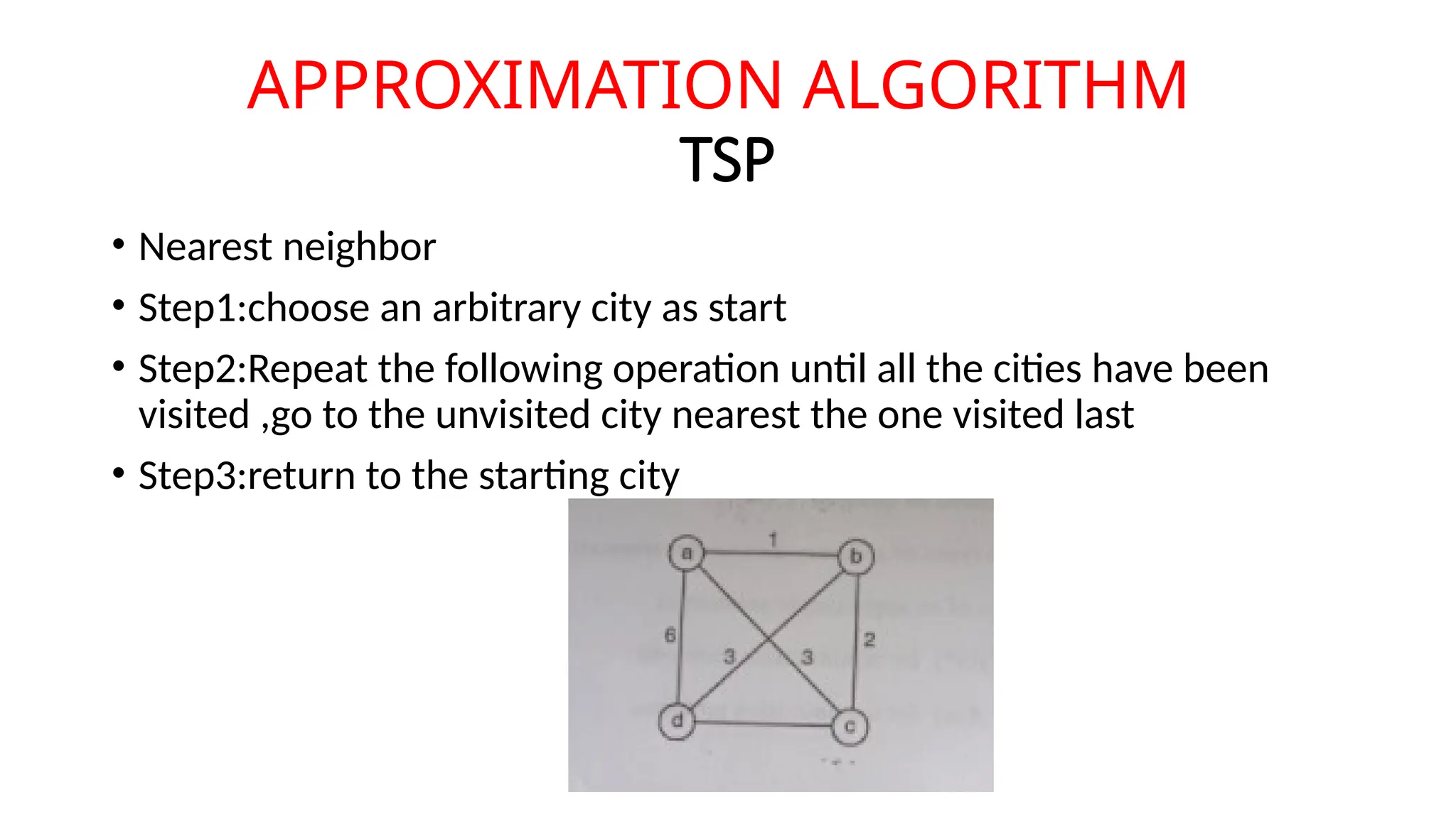
APPROXIMATION ALGORITHM
TSP
• Nearest neighbor
• Step1:choose an arbitrary city as start
• Step2:Repeat the following operation until all the cities have been
visited ,go to the unvisited city nearest the one visited last
• Step3:return to the starting city

• Sa=a-b-c-d-a=1+2+1+6=10
• a-c-b-d-a=3+2+3+6=14
• a-c-d-b-a=3+1+3+1=8

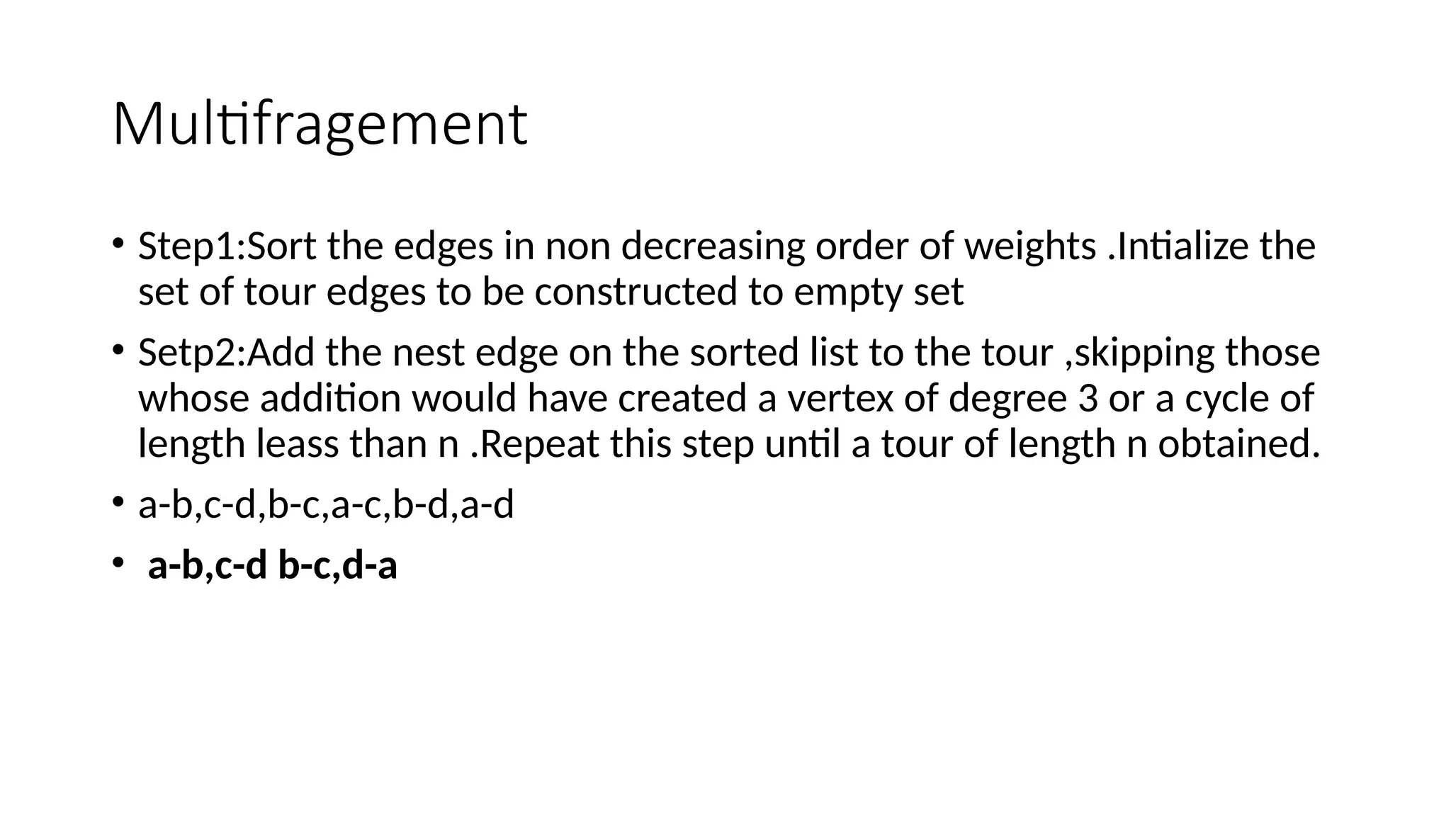
Multifragement
• Step1:Sort the edges in non decreasing order of weights .Intialize the
set of tour edges to be constructed to empty set
• Setp2:Add the nest edge on the sorted list to the tour ,skipping those
whose addition would have created a vertex of degree 3 or a cycle of
length leass than n .Repeat this step until a tour of length n obtained.
• a-b,c-d,b-c,a-c,b-d,a-d
• a-b,c-d b-c,d-a

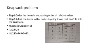
Knapsack problem
• Step1:Order the items in decreasing order of relative values
• Step2:Select the items in this order skipping those that don’t fit into
the knapsack.
• Knapsack Capacity:16
• I1,I2,I4,I3
• I1,I2,I3=2+5+5=12

Approximation scheme for knapsack problem

Randomized Algorithm
What is Randomized Algorithm?
An algorithm that uses random numbers to decide what to do next anywhere in its
logic is called Randomized Algorithm.
For example, in Randomized Quick Sort, we use a random number to pick the next
pivot (or we randomly shuffle the array).
Typically, this randomness is used to reduce time complexity or space complexity in
other standard algorithms.

Randomized Quick Sort Algorithm
• The algorithm exactly follows the standard algorithm except it
randomizes the pivot selection.

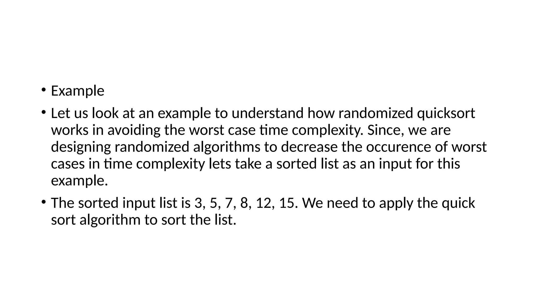
• Example
• Let us look at an example to understand how randomized quicksort
works in avoiding the worst case time complexity. Since, we are
designing randomized algorithms to decrease the occurence of worst
cases in time complexity lets take a sorted list as an input for this
example.
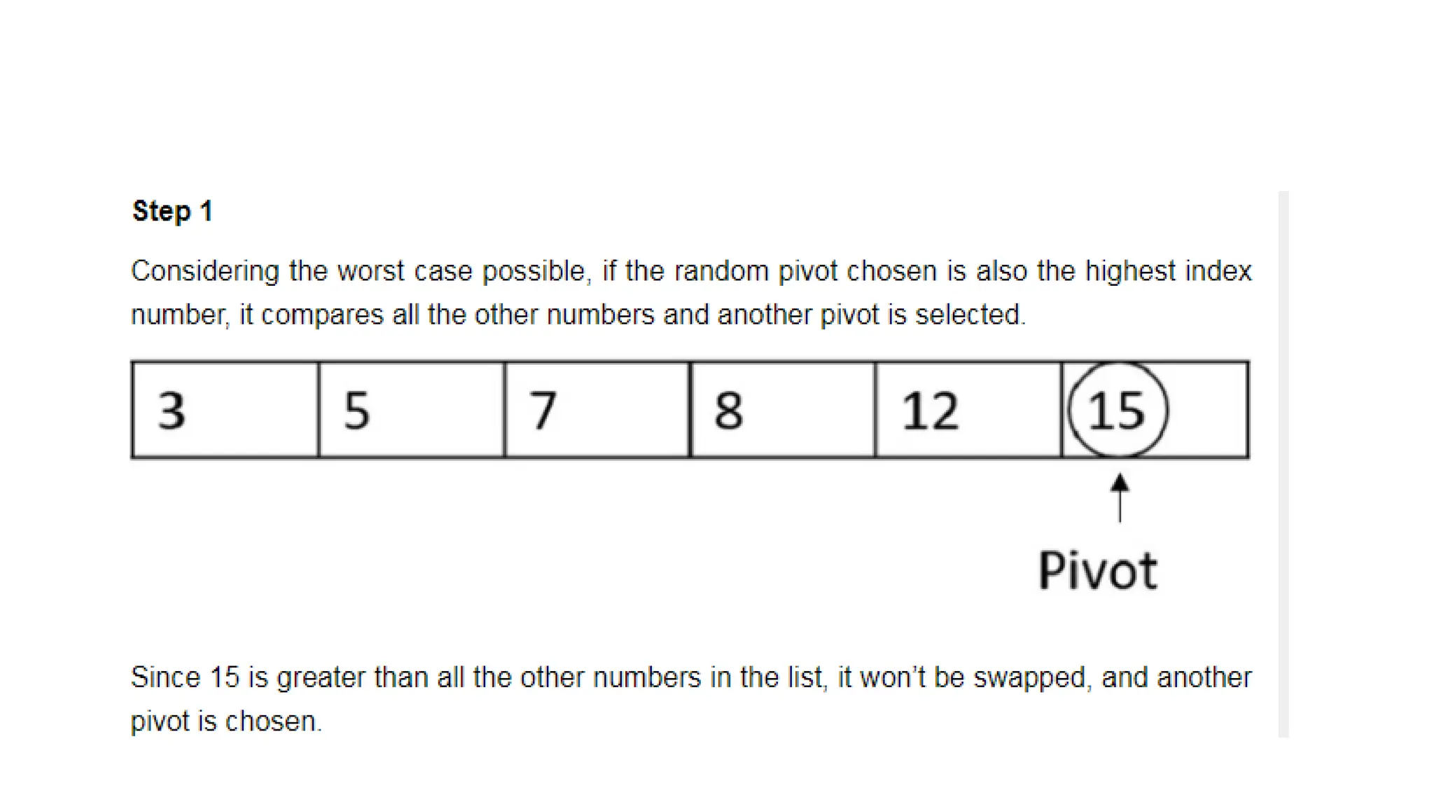
• The sorted input list is 3, 5, 7, 8, 12, 15. We need to apply the quick
sort algorithm to sort the list.

optimal merge pattern notes - algorithms

More Related Content

Similar to optimal merge pattern notes - algorithms

Recently uploaded

optimal merge pattern notes - algorithms