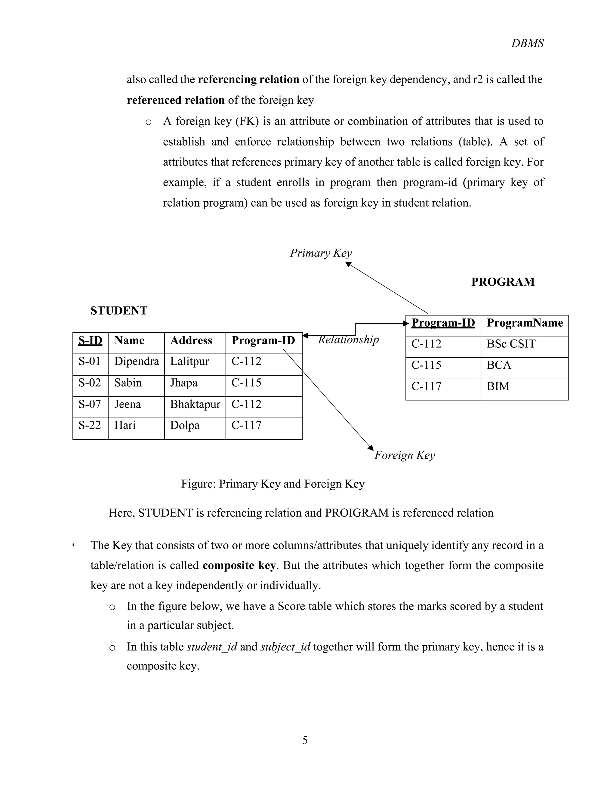
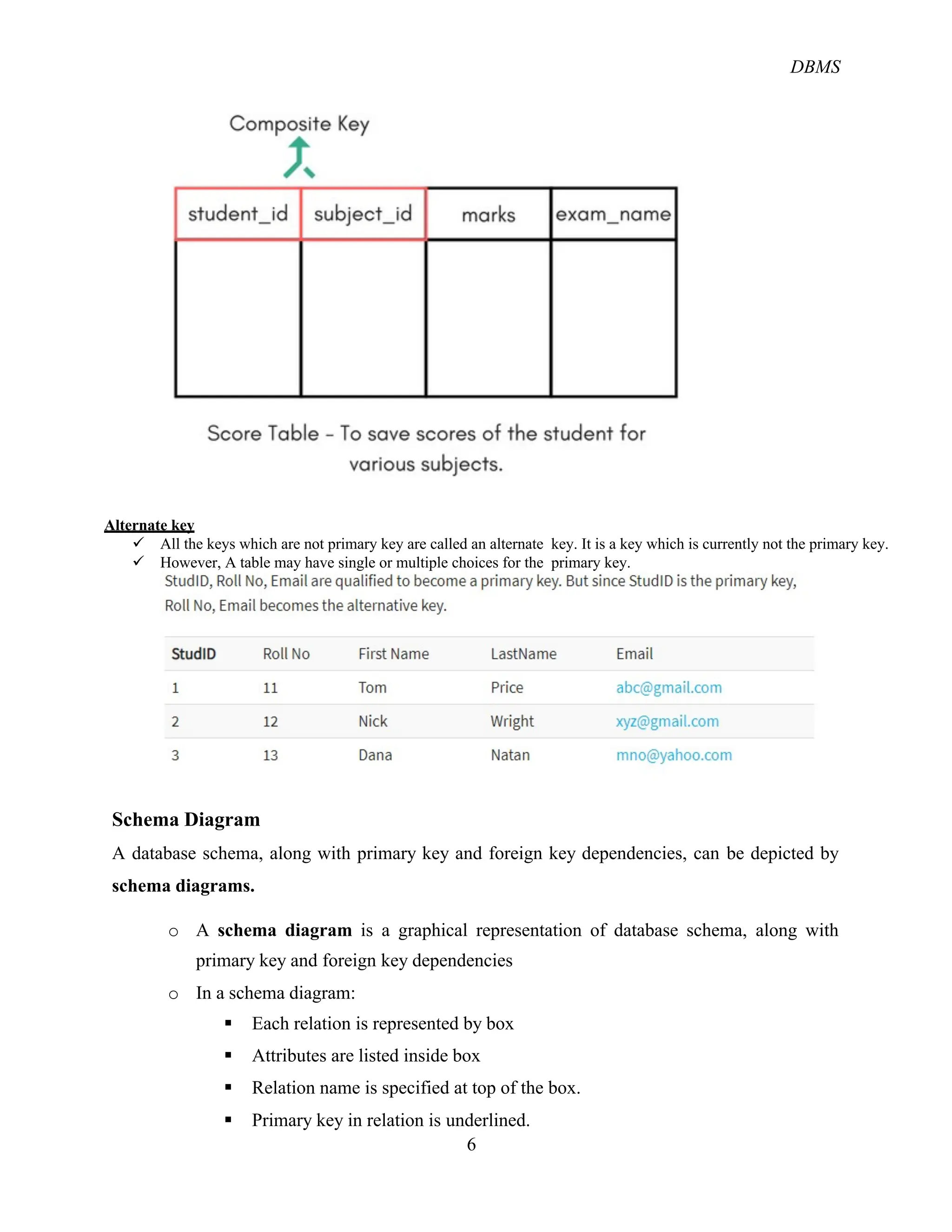
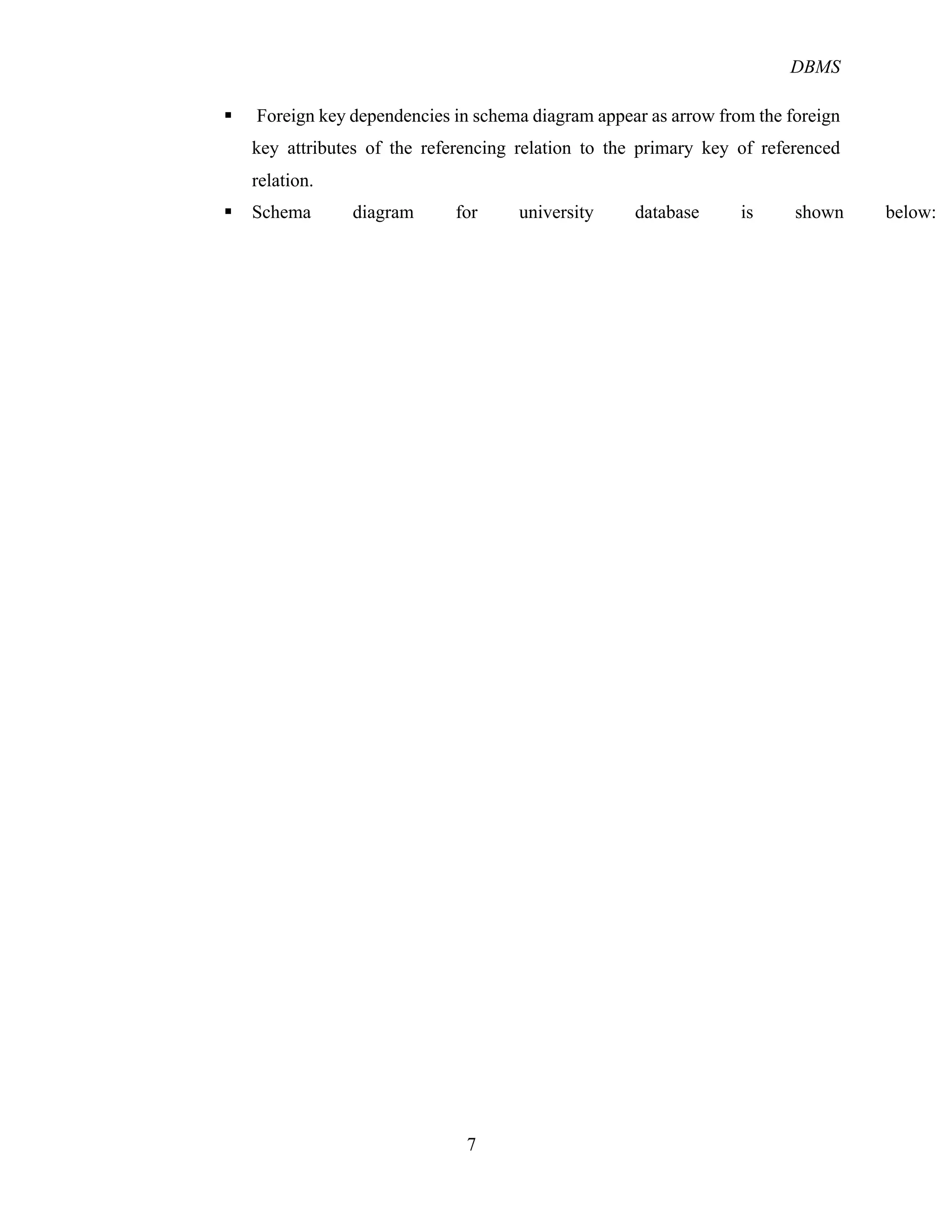
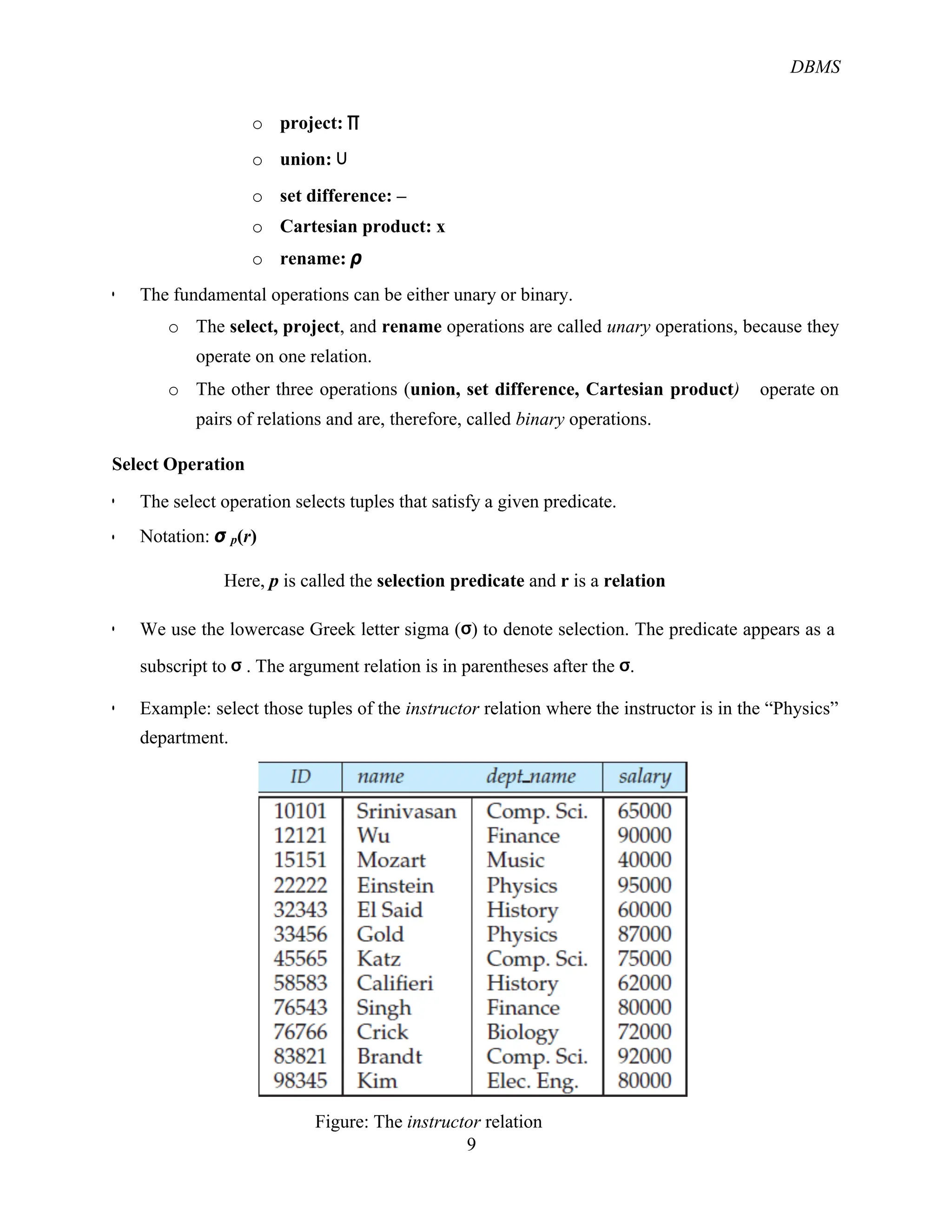
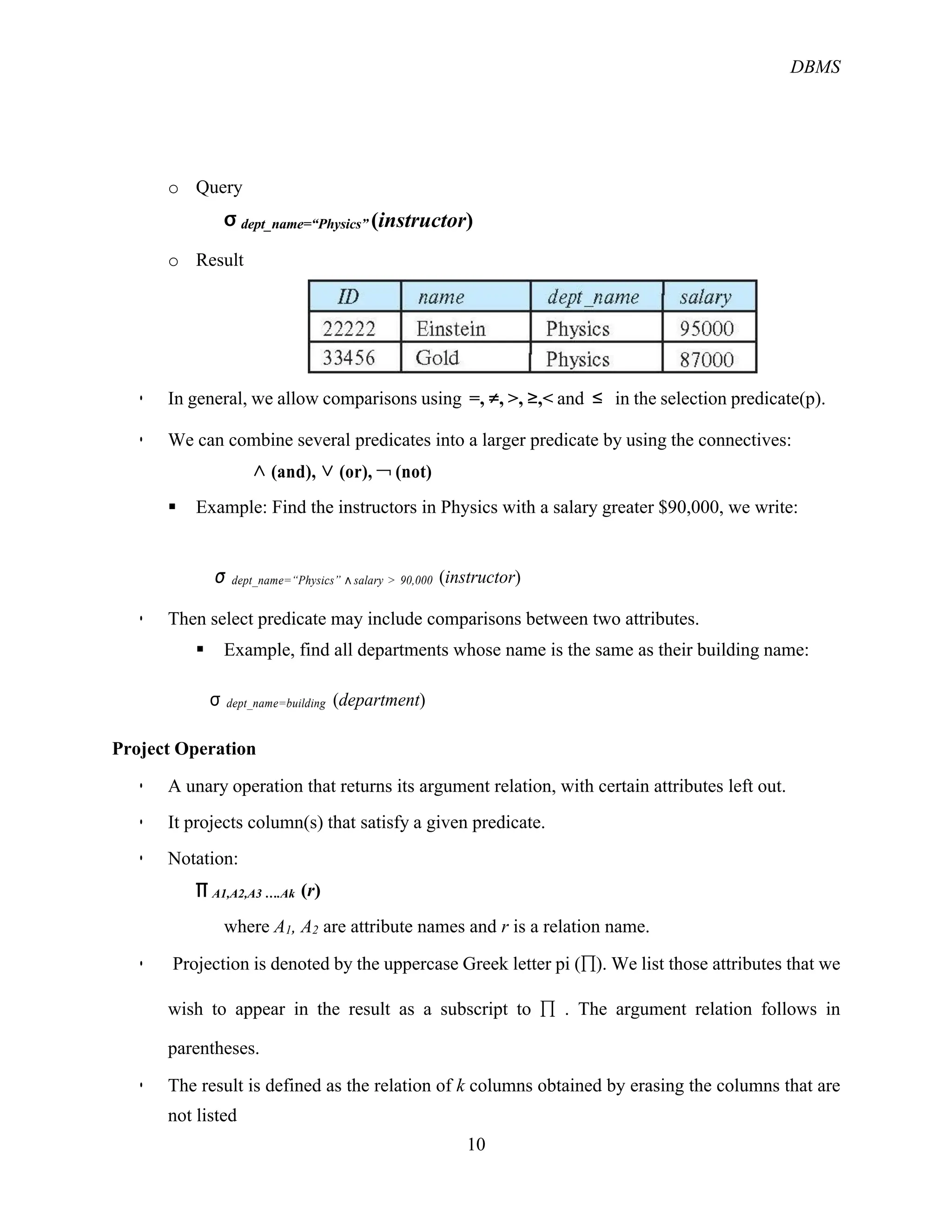
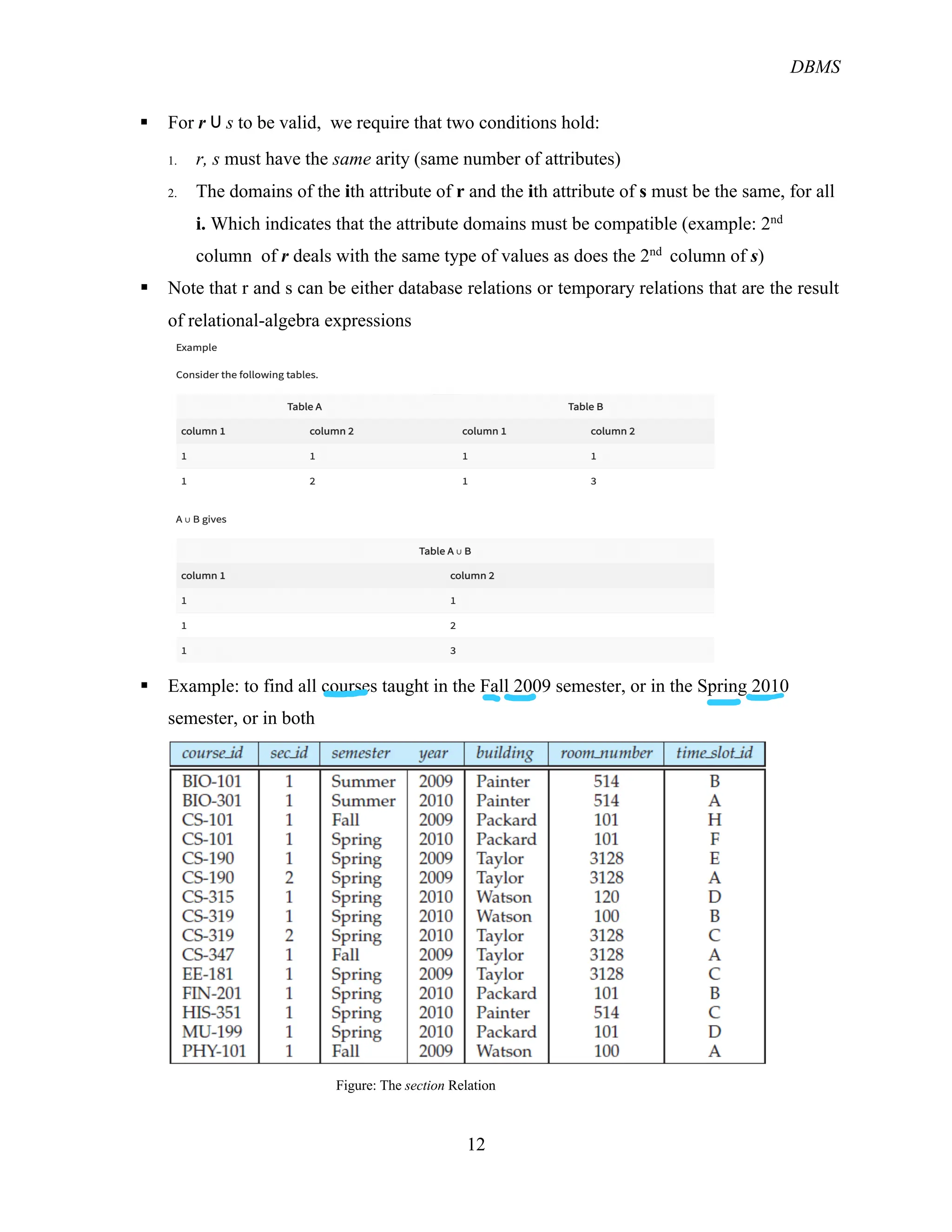
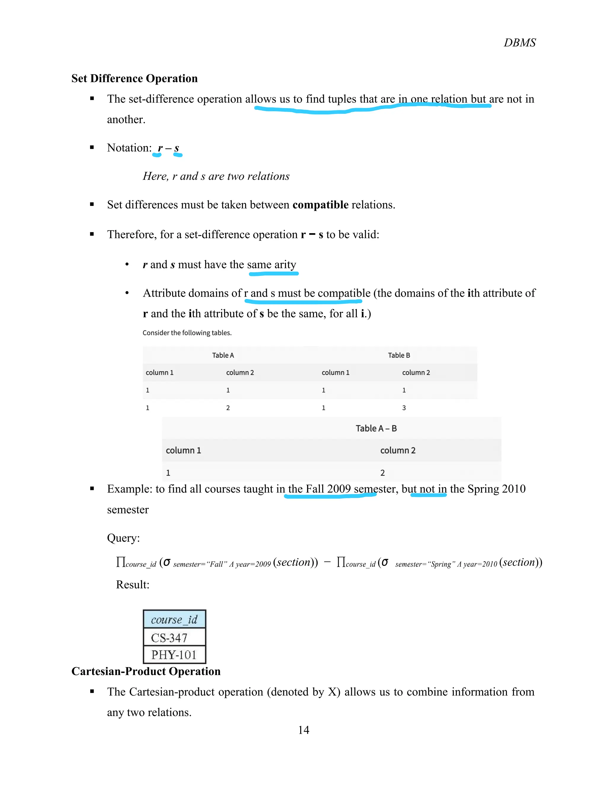
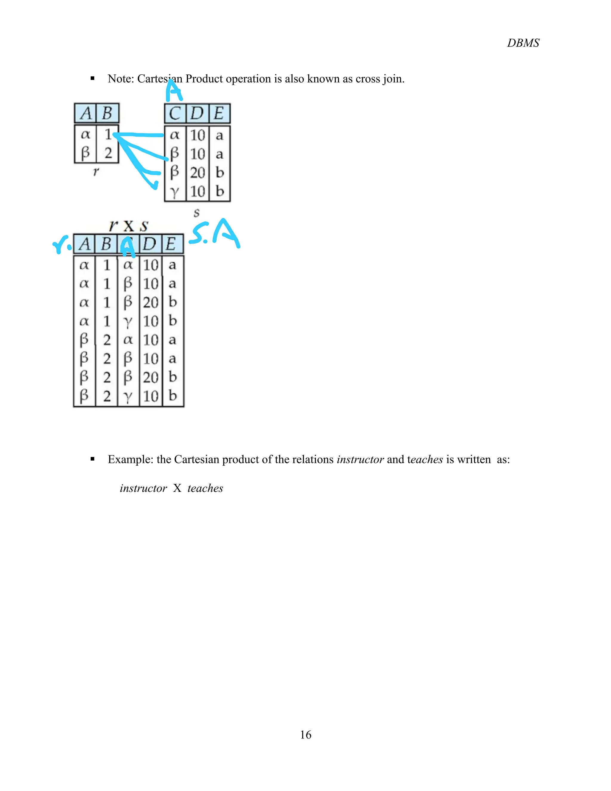
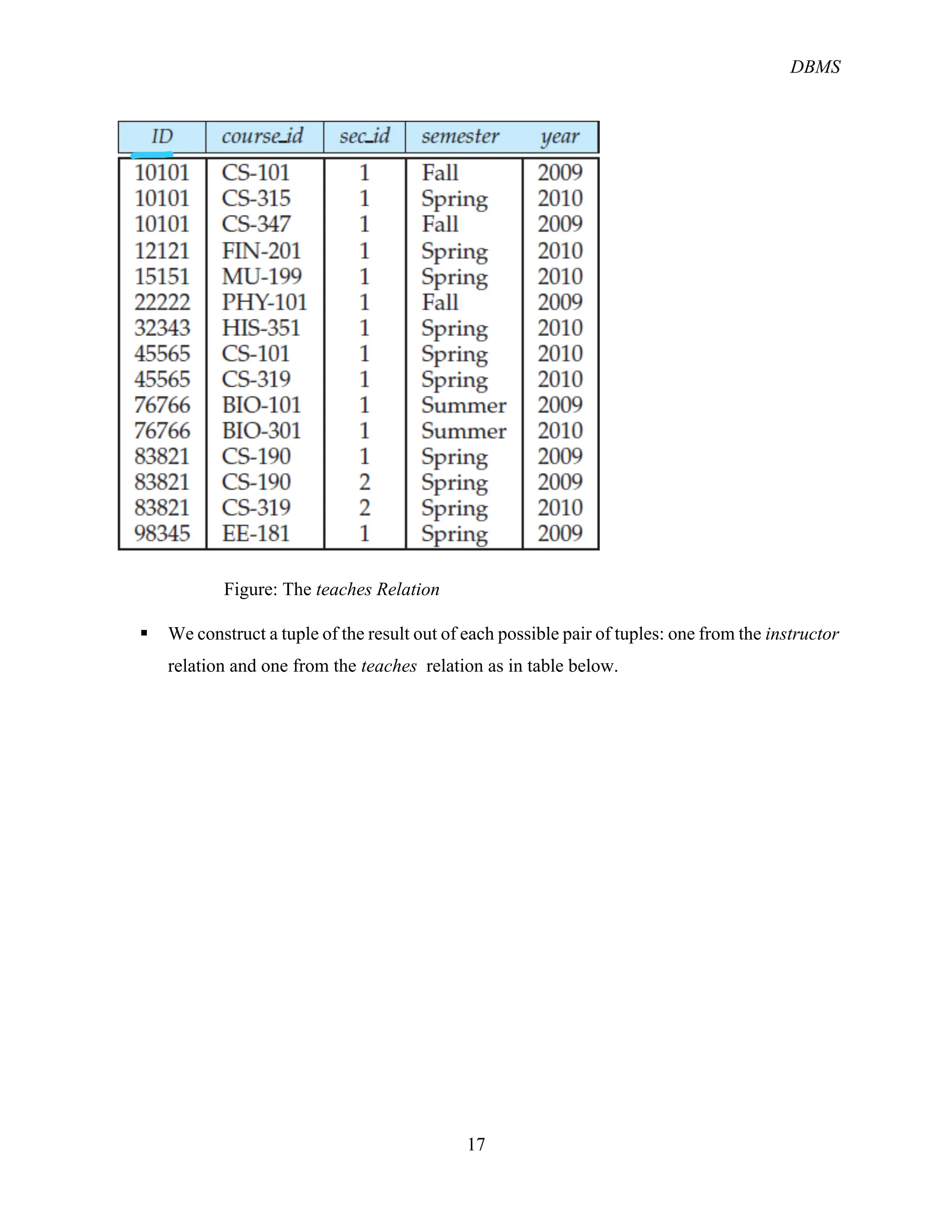
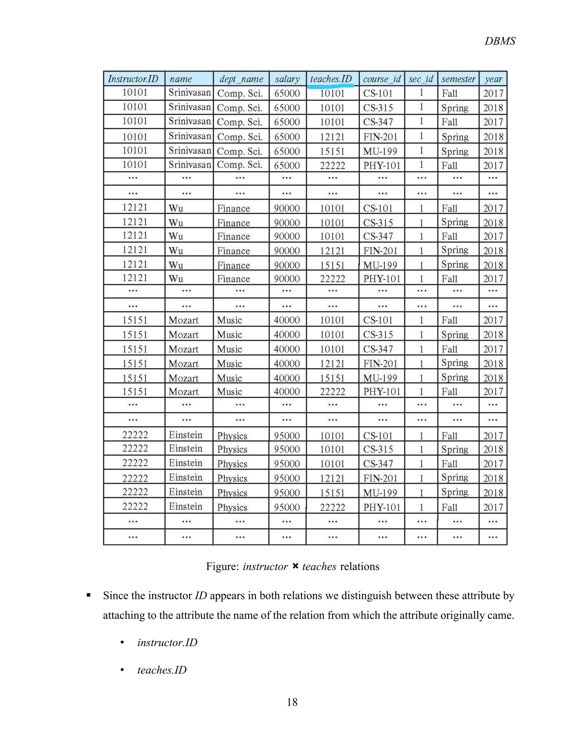
KEMBAR78
Relational Database Model Database Management system | PDF
DBMS
1
Unit -3: Relational Database Model
Structure of RDBMS and Terminology
! RDBMS = Relational Database Management System
! The relational model is today the primary data model for commercial data processing
applications. It attained its primary position because of its simplicity. It provides simple
but powerful way of representing data.
! Relational model is simply a collection of one or more relations, where each relation is
represented by table with rows and columns.
! It is the most widely used data model. The relational model uses a collection of tables to
represent both data and the relationships among those data. Each table has multiple
columns, and each column has a unique name. Tables are known as relations. Each table
corresponds to an entity set or relationship set, and each row represents an instance of that
entity set or relationship set. Relationships link rows from two tables by embedding row
identifiers (keys) from one table as attribute values in the other table. Structured Query
Language (SQL) is used to manipulate data stored in tables.
Table (Relation) Attributes / Fields/Columns
Record /Tuple/Row
Data Values
CustomerId CustomerName CustomerAddress
202 Priya Kathmandu
203 Baburam Lalitpur
204 Suntali Bhaktapur
205 Nabin Kathmandu
206 Krishna Pokhara
DBMS
2
! A relational database consists of a collection of tables, each of which is assigned a unique
name.
! In the relational model the term relation is used to refer to a table, while the term tuple is
used to refer to a row. Similarly, the term attribute refers to a column of a table.
! We use the term relation instance to refer to a specific instance of a relation, i.e., containing
a specific set of rows.
! Order of tuples is irrelevant (tuples may be stored in an arbitrary order)
! For each attribute of a relation, there is a set of permitted values, called the domain of that
attribute. Thus, the domain of the salary attribute of the instructor relation is the set of all
possible salary values, while the domain of the name attribute is the set of all possible
instructor names.
! Attribute values are (normally) required to be atomic; that is, indivisible
! A domain is said to be atomic if elements of the domain are considered to be indivisible
units. Domains of multivalued and composite attributes are non atomic.
! The null value is a special value that signifies that the value is unknown or does not exist.
! The special value null is a member of every domain
Relation schema and instance
! Database schema, is the logical design of the database, and the database instance is a
snapshot of the data in the database at a given instant in time.
! In general, a relation schema consists of a list of attributes and their corresponding
domains.
! A1, A2, …, An are attributes
! R = (A1, A2, …, An ) is a relation schema
Example:
instructor = (ID, name, dept_name, salary)
! Formally, given sets D1, D2, …. Dn a relation r is a subset of
D1 x D2 x … x Dn
Thus, a relation is a set of n-tuples (a1, a2, …, an) where each ai "#Di
! The current values (relation instance) of a relation are specified by a table
DBMS
3
! An element t of r is a tuple, represented by a row in a table
! Relational Schemas for university database:
o instructor (ID, name, dept_name, salary)
o department (dept _name, building, budget)
o section (course _id, sec _id, semester, year, building, room_ number, time _slot_ id)
o prereq (course _id, prereq_ id)
o teaches (ID, course_ id, sec _id, semester, year)
o student (ID, name, dept _name, tot _cred)
o advisor (s_ id, i_ id)
o takes (ID, course _id, sec_ id, semester, year, grade)
o classroom (building, room number, capacity)
o time _slot (time _slot _id, day, start _time, end _time)
Keys (super key, candidate key, primary key, foreign key, composite key, alternative key)
! Keys are used to uniquely identify the tuples in a relations.
! No two tuples in a relation are allowed to have exactly the same value for all attributes.
! Let K $#R
! K is a superkey of R if values for K are sufficient to identify a unique tuple of each
possible relation r(R)
o A superkey is a set of one or more attributes that, taken collectively, allow us
to identify uniquely a tuple in the relation
o Example: {ID} and {ID,name} are both superkeys of instructor.
! We are often interested in superkeys for which no proper subset is a superkey. Such
minimal superkeys are called candidate keys
o A super key with no repeated attribute is called candidate key.
o The Primary key should be selected from the candidate keys. Every table
must have at least a single candidate key.
o Superkey K is a candidate key if K is minimal
Example: {ID} is a candidate key for instructor
Properties of Candidate key:
o It must contain unique values
o Candidate key may have multiple attributes
DBMS
4
o Must not contain null values
o It should contain minimum fields to ensure
uniqueness
o Uniquely identify each record in a table
! One of the candidate keys is selected to be the primary key.
o The primary key is candidate key that is chosen by the database designer as
the principal means of identifying tuples within a relation
Rules for defining Primary key:
o Two rows can't have the same primary key value
o It must for every row to have a primary key value.
o The primary key field cannot be null.
o The value in a primary key column can never be modified or updated if any
foreign key
o refers to that primary key.
! A relation, say r1, may include among its attributes the primary key of another relation,
say r2. This attribute is called a foreign key from r1, referencing r2. The relation r1 is
DBMS
5
also called the referencing relation of the foreign key dependency, and r2 is called the
referenced relation of the foreign key
o A foreign key (FK) is an attribute or combination of attributes that is used to
establish and enforce relationship between two relations (table). A set of
attributes that references primary key of another table is called foreign key. For
example, if a student enrolls in program then program-id (primary key of
relation program) can be used as foreign key in student relation.
Primary Key
PROGRAM
STUDENT
S-ID Name Address Program-ID
S-01 Dipendra Lalitpur C-112
S-02 Sabin Jhapa C-115
S-07 Jeena Bhaktapur C-112
S-22 Hari Dolpa C-117
Foreign Key
Figure: Primary Key and Foreign Key
Here, STUDENT is referencing relation and PROIGRAM is referenced relation
! The Key that consists of two or more columns/attributes that uniquely identify any record in a
table/relation is called composite key. But the attributes which together form the composite
key are not a key independently or individually.
o In the figure below, we have a Score table which stores the marks scored by a student
in a particular subject.
o In this table student_id and subject_id together will form the primary key, hence it is a
composite key.
Relationship
Program-ID ProgramName
C-112 BSc CSIT
C-115 BCA
C-117 BIM
DBMS
6
Alternate key
ü All the keys which are not primary key are called an alternate key. It is a key which is currently not the primary key.
ü However, A table may have single or multiple choices for the primary key.
Schema Diagram
A database schema, along with primary key and foreign key dependencies, can be depicted by
schema diagrams.
o A schema diagram is a graphical representation of database schema, along with
primary key and foreign key dependencies
o In a schema diagram:
§ Each relation is represented by box
§ Attributes are listed inside box
§ Relation name is specified at top of the box.
§ Primary key in relation is underlined.
DBMS
7
§ Foreign key dependencies in schema diagram appear as arrow from the foreign
key attributes of the referencing relation to the primary key of referenced
relation.
§ Schema diagram for university database is shown below:
DBMS
8
Figure: Schema diagram for university database
Introduction to Relational Algebra
! The relational algebra is a procedural query language. It consists of a set of operations that
take one or two relations as input and produce a new relation as their result.
! The fundamental operations in the relational algebra are select, project, union, set
difference, Cartesian product, and rename.
! In addition to the fundamental operations, there are several other operations—namely, set
intersection, natural join, and assignment. We shall define these operations in terms of the
fundamental operations.
Fundamental Operations in Relational Algebra (RA):
! There are six fundamental (basic) operations /operators as follows:
o select: σ
DBMS
9
o project: ∏
o union: ∪
o set difference: –
o Cartesian product: x
o rename: ρ
! The fundamental operations can be either unary or binary.
o The select, project, and rename operations are called unary operations, because they
operate on one relation.
o The other three operations (union, set difference, Cartesian product) operate on
pairs of relations and are, therefore, called binary operations.
Select Operation
! The select operation selects tuples that satisfy a given predicate.
! Notation: σ p(r)
Here, p is called the selection predicate and r is a relation
! We use the lowercase Greek letter sigma (σ) to denote selection. The predicate appears as a
subscript to σ . The argument relation is in parentheses after the σ.
! Example: select those tuples of the instructor relation where the instructor is in the “Physics”
department.
Figure: The instructor relation
DBMS
10
o Query
σ dept_name=“Physics” (instructor)
o Result
! In general, we allow comparisons using =, ≠, >, ≥,< and ≤ in the selection predicate(p).
! We can combine several predicates into a larger predicate by using the connectives:
∧ (and), ∨ (or), ¬ (not)
§ Example: Find the instructors in Physics with a salary greater $90,000, we write:
σ dept_name=“Physics” !"salary > 90,000 (instructor)
! Then select predicate may include comparisons between two attributes.
§ Example, find all departments whose name is the same as their building name:
%#dept_name=building (department)
Project Operation
! A unary operation that returns its argument relation, with certain attributes left out.
! It projects column(s) that satisfy a given predicate.
! Notation:
∏ A1,A2,A3 ….Ak (r)
where A1, A2 are attribute names and r is a relation name.
! Projection is denoted by the uppercase Greek letter pi (&). We list those attributes that we
wish to appear in the result as a subscript to &# . The argument relation follows in
parentheses.
! The result is defined as the relation of k columns obtained by erasing the columns that are
not listed
DBMS
11
! Duplicate rows are removed from result, since relations are sets.
! Example: eliminate the dept_name attribute of instructor
! Query:
Result:
&ID, name, salary (instructor)
Composition of Relational Operations
§ The result of a relational-algebra operation is relation and therefore of relational-algebra
operations can be composed together into a relational-algebra expression.
§ Consider the query – Find the names of all instructors in the Physics department.
&name(σ dept_name =“Physics” (instructor))
§ Instead of giving the name of a relation as the argument of the projection operation, we
give an expression that evaluates to a relation.
Union Operation
§ The union operation allows us to combine two relations.
§ Notation: r ∪ s
Here, r and s are two relations
DBMS
12
§ For r ∪ s to be valid, we require that two conditions hold:
1. r, s must have the same arity (same number of attributes)
2. The domains of the ith attribute of r and the ith attribute of s must be the same, for all
i. Which indicates that the attribute domains must be compatible (example: 2nd
column of r deals with the same type of values as does the 2nd
column of s)
§ Note that r and s can be either database relations or temporary relations that are the result
of relational-algebra expressions
§ Example: to find all courses taught in the Fall 2009 semester, or in the Spring 2010
semester, or in both
Figure: The section Relation
DBMS
13
Query:
&course_id (%#semester=“Fall” Λ year=2009 (section)) '#&course_id (%#semester=“Spring” Λ year=2010 (section))
The query gives above table as a Result.
DBMS
14
Set Difference Operation
§ The set-difference operation allows us to find tuples that are in one relation but are not in
another.
§ Notation: r – s
Here, r and s are two relations
§ Set differences must be taken between compatible relations.
§ Therefore, for a set-difference operation r − s to be valid:
• r and s must have the same arity
• Attribute domains of r and s must be compatible (the domains of the ith attribute of
r and the ith attribute of s be the same, for all i.)
§ Example: to find all courses taught in the Fall 2009 semester, but not in the Spring 2010
semester
Query:
&course_id (σ semester=“Fall” Λ year=2009 (section)) − &course_id (σ semester=“Spring” Λ year=2010 (section))
Result:
Cartesian-Product Operation
§ The Cartesian-product operation (denoted by X) allows us to combine information from
any two relations.
DBMS
15
§ We write the Cartesian product of relations r1 and r2 as r = r1 × r2.
§ In general, if we have relations r1(R1) and r2(R2), then r1 × r2 is a relation whose schema
is the concatenation of R1 and R2.
DBMS
16
§ Note: Cartesian Product operation is also known as cross join.
§ Example: the Cartesian product of the relations instructor and teaches is written as:
instructor X teaches
DBMS
17
Figure: The teaches Relation
§ We construct a tuple of the result out of each possible pair of tuples: one from the instructor
relation and one from the teaches relation as in table below.
DBMS
18
Figure: instructor × teaches relations
§ Since the instructor ID appears in both relations we distinguish between these attribute by
attaching to the attribute the name of the relation from which the attribute originally came.
• instructor.ID
• teaches.ID
DBMS
19
The Rename Operation
§ The results of relational-algebra expressions do not have a name that we can use to refer to
them. The rename operator, denoted by the lowercase Greek letter rho (ρ), ρ , is provided for
that purpose.
The expression: ρx (E)
returns the result of expression E under the name x
§ Another form of the rename operation:
ρx(A1,A2, .. An) (E)
returns the result of expression E under the name x, and with the attributes renamed
to A1, A2, . . . , An
Types of JOIN
Various forms of join operation are:
Inner Joins:
• Theta join
• EQUI join
• Natural join
Outer join:
• Left Outer Join
• Right Outer Join
• Full Outer Join
Natural-Join Operation
§ The natural join is a binary operation that allows us to combine certain selections and a
Cartesian product into one operation.
§ It is denoted by the join symbol ⋈.
§ The natural-join operation forms a Cartesian product of its two arguments, performs a
selection forcing equality on those attributes that appear in both relation schemas, and
finally removes duplicate attributes
§ Returning to the example of the relations instructor and teaches, computing instructor
natural join teaches considers only those pairs of tuples where both the tuple from
DBMS
20
instructor and the tuple from teaches have the same value on the common attribute ID.The
result is shown in following figure.
§ Notice that we do not repeat those attributes that appear in the schemas of both relations;
rather they appear only once. Notice also the order in which the attributes are listed:
o first the attributes common to the schemas of both relations,
o second those attributes unique to the schema of the first relation,
o and finally, those attributes unique to the schema of the second relation
DBMS
21
Figure : The natural join of the instructor relation with the teaches relation
§ The natural join of r and s, denoted by r ⋈ s, is a relation on schema R ∪ S formally defined
as follows:
Where R ∩ S = {A1, A2, . . . , An}.
§ If r (R) and s(S) are relations without any attributes in common, that is, R ∩ S = ∅, then
r ⋈ s = r × s.
DBMS
22
DBMS
23
§ The theta join operation is a variant of the natural-join operation that allows us to combine
a selection and a Cartesian product into a single operation. Consider relations r (R) and
s(S), and let 𝜃 be a predicate on attributes in the schema R ∪ S. The theta join operation
r ⋈𝜽
s is defined as follows:
𝑟 ⋈𝜃
𝑠 = 𝜎𝜃
(𝑟 × 𝑠)
Thus, %# instructor.id = teaches.id (instructor x teaches)
Can equivalently be written as:
instructor ⋈ Instructor.id = teaches.id teaches.
Equi join operation
§ When a theta join uses only equivalence condition, it becomes a equi join.
Outer join Operations
§ The outer-join operation is an extension of the join operation to deal with missing
information.
§ The outer join operation works in a manner similar to the natural join operation, but
preserves those tuples that would be lost in an join by creating tuples in the result containing
null values
§ We can use the outer-join operation to avoid this loss of information.
§ There are actually three forms of the operation:
o left outer join (denoted as )
o right outer join (denoted as )
DBMS
24
o full outer join (denoted as )
§ The left outer join takes all tuples in the left relation that did not match with any tuple in
the right relation, pads the tuples with null values for all other attributes from the right
relation, and adds them to the result of the natural join.
o Takes all tuples in the left relation. If there are any tuples in right relation that does
not match with tuple in left relation, simply pads these right relation tuples with
null.
§ The right outer join is symmetric with the left outer join: It pads tuples from the right
relation that did not match any from the left relation with nulls and adds them to the result
of the natural join
o Takes all tuples in right relation. If there are any tuples in the left relation that does
not match with tuples in right relation, simply pads relation tuples with null.
§ The full outer join does both the left and right outer join operations, padding tuples from
the left relation that did not match any from the right relation, as well as tuples from the
right relation that did not match any from the left relation, and adding them to the result of
the join.
o Pads tuples from the left relation that did not match any from the right relation.
o Pads tuples from the left relation that did not match any from the left relation
DBMS
25
Left outer join
Right outer join
Full outer join
DBMS
26
Example: Consider two relations loan and borrow. Different join operations on these relations are
shown in figures below.
DBMS
27
Summary
Operation(Symbols) Purpose
Select(σ)
The SELECT operation is used for selecting a
subset of the tuples according to a given
selection condition
Projection(π)
The projection eliminates all attributes of the
input relation but those mentioned in the
projection list.
Union Operation(∪)
UNION is symbolized by symbol. It includes
all tuples that are in tables A or in B.
Set Difference(-)
– Symbol denotes it. The result of A – B, is a
relation which includes all tuples that are in A
but not in B.
Intersection(∩)
Intersection defines a relation consisting of a
set of all tuple that are in both A and B.
Cartesian Product(X)
Cartesian operation is helpful to merge
columns from two relations.
DBMS
28
Inner Join
Inner join, includes only those tuples that
satisfy the matching criteria.
Theta Join(θ)
The general case of JOIN operation is called a
Theta join. It is denoted by symbol θ.
EQUI Join
When a theta join uses only equivalence
condition, it becomes a equi join.
Natural Join(⋈)
Natural join can only be performed if there is
a common attribute (column) between the
relations.
Outer Join
In an outer join, along with tuples that satisfy
the matching criteria.
Left Outer Join( )
In the left outer join, operation allows
keeping all tuple in the left relation.
Right Outer join( )
In the right outer join, operation allows
keeping all tuple in the right relation.
Full Outer Join( )
In a full outer join, all tuples from both
relations are included in the result
irrespective of the matching condition.
DBMS
29
Exercise :
1. Find all tuples from player relation for which country is India.
2. Select all the tuples for which runs are greater than or equal to 15000.
3. Select all the players whose runs are greater than or equal to 6000 and age is less than 25
4. List all the countries in Player relation.
5. List all the team ids and countries in Player Relation.
6. Find all the customers having an account but not the loan.
7. Find all the customers having a loan but not the account.
8. Rename Customer relation to CustomerList.

Relational Database Model Database Management system

  • 1.
    DBMS 1 Unit -3: RelationalDatabase Model Structure of RDBMS and Terminology ! RDBMS = Relational Database Management System ! The relational model is today the primary data model for commercial data processing applications. It attained its primary position because of its simplicity. It provides simple but powerful way of representing data. ! Relational model is simply a collection of one or more relations, where each relation is represented by table with rows and columns. ! It is the most widely used data model. The relational model uses a collection of tables to represent both data and the relationships among those data. Each table has multiple columns, and each column has a unique name. Tables are known as relations. Each table corresponds to an entity set or relationship set, and each row represents an instance of that entity set or relationship set. Relationships link rows from two tables by embedding row identifiers (keys) from one table as attribute values in the other table. Structured Query Language (SQL) is used to manipulate data stored in tables. Table (Relation) Attributes / Fields/Columns Record /Tuple/Row Data Values CustomerId CustomerName CustomerAddress 202 Priya Kathmandu 203 Baburam Lalitpur 204 Suntali Bhaktapur 205 Nabin Kathmandu 206 Krishna Pokhara
  • 2.
    DBMS 2 ! A relationaldatabase consists of a collection of tables, each of which is assigned a unique name. ! In the relational model the term relation is used to refer to a table, while the term tuple is used to refer to a row. Similarly, the term attribute refers to a column of a table. ! We use the term relation instance to refer to a specific instance of a relation, i.e., containing a specific set of rows. ! Order of tuples is irrelevant (tuples may be stored in an arbitrary order) ! For each attribute of a relation, there is a set of permitted values, called the domain of that attribute. Thus, the domain of the salary attribute of the instructor relation is the set of all possible salary values, while the domain of the name attribute is the set of all possible instructor names. ! Attribute values are (normally) required to be atomic; that is, indivisible ! A domain is said to be atomic if elements of the domain are considered to be indivisible units. Domains of multivalued and composite attributes are non atomic. ! The null value is a special value that signifies that the value is unknown or does not exist. ! The special value null is a member of every domain Relation schema and instance ! Database schema, is the logical design of the database, and the database instance is a snapshot of the data in the database at a given instant in time. ! In general, a relation schema consists of a list of attributes and their corresponding domains. ! A1, A2, …, An are attributes ! R = (A1, A2, …, An ) is a relation schema Example: instructor = (ID, name, dept_name, salary) ! Formally, given sets D1, D2, …. Dn a relation r is a subset of D1 x D2 x … x Dn Thus, a relation is a set of n-tuples (a1, a2, …, an) where each ai "#Di ! The current values (relation instance) of a relation are specified by a table
  • 3.
    DBMS 3 ! An elementt of r is a tuple, represented by a row in a table ! Relational Schemas for university database: o instructor (ID, name, dept_name, salary) o department (dept _name, building, budget) o section (course _id, sec _id, semester, year, building, room_ number, time _slot_ id) o prereq (course _id, prereq_ id) o teaches (ID, course_ id, sec _id, semester, year) o student (ID, name, dept _name, tot _cred) o advisor (s_ id, i_ id) o takes (ID, course _id, sec_ id, semester, year, grade) o classroom (building, room number, capacity) o time _slot (time _slot _id, day, start _time, end _time) Keys (super key, candidate key, primary key, foreign key, composite key, alternative key) ! Keys are used to uniquely identify the tuples in a relations. ! No two tuples in a relation are allowed to have exactly the same value for all attributes. ! Let K $#R ! K is a superkey of R if values for K are sufficient to identify a unique tuple of each possible relation r(R) o A superkey is a set of one or more attributes that, taken collectively, allow us to identify uniquely a tuple in the relation o Example: {ID} and {ID,name} are both superkeys of instructor. ! We are often interested in superkeys for which no proper subset is a superkey. Such minimal superkeys are called candidate keys o A super key with no repeated attribute is called candidate key. o The Primary key should be selected from the candidate keys. Every table must have at least a single candidate key. o Superkey K is a candidate key if K is minimal Example: {ID} is a candidate key for instructor Properties of Candidate key: o It must contain unique values o Candidate key may have multiple attributes
  • 4.
    DBMS 4 o Must notcontain null values o It should contain minimum fields to ensure uniqueness o Uniquely identify each record in a table ! One of the candidate keys is selected to be the primary key. o The primary key is candidate key that is chosen by the database designer as the principal means of identifying tuples within a relation Rules for defining Primary key: o Two rows can't have the same primary key value o It must for every row to have a primary key value. o The primary key field cannot be null. o The value in a primary key column can never be modified or updated if any foreign key o refers to that primary key. ! A relation, say r1, may include among its attributes the primary key of another relation, say r2. This attribute is called a foreign key from r1, referencing r2. The relation r1 is
  • 5.
    DBMS 5 also called thereferencing relation of the foreign key dependency, and r2 is called the referenced relation of the foreign key o A foreign key (FK) is an attribute or combination of attributes that is used to establish and enforce relationship between two relations (table). A set of attributes that references primary key of another table is called foreign key. For example, if a student enrolls in program then program-id (primary key of relation program) can be used as foreign key in student relation. Primary Key PROGRAM STUDENT S-ID Name Address Program-ID S-01 Dipendra Lalitpur C-112 S-02 Sabin Jhapa C-115 S-07 Jeena Bhaktapur C-112 S-22 Hari Dolpa C-117 Foreign Key Figure: Primary Key and Foreign Key Here, STUDENT is referencing relation and PROIGRAM is referenced relation ! The Key that consists of two or more columns/attributes that uniquely identify any record in a table/relation is called composite key. But the attributes which together form the composite key are not a key independently or individually. o In the figure below, we have a Score table which stores the marks scored by a student in a particular subject. o In this table student_id and subject_id together will form the primary key, hence it is a composite key. Relationship Program-ID ProgramName C-112 BSc CSIT C-115 BCA C-117 BIM
  • 6.
    DBMS 6 Alternate key ü Allthe keys which are not primary key are called an alternate key. It is a key which is currently not the primary key. ü However, A table may have single or multiple choices for the primary key. Schema Diagram A database schema, along with primary key and foreign key dependencies, can be depicted by schema diagrams. o A schema diagram is a graphical representation of database schema, along with primary key and foreign key dependencies o In a schema diagram: § Each relation is represented by box § Attributes are listed inside box § Relation name is specified at top of the box. § Primary key in relation is underlined.
  • 7.
    DBMS 7 § Foreign keydependencies in schema diagram appear as arrow from the foreign key attributes of the referencing relation to the primary key of referenced relation. § Schema diagram for university database is shown below:
  • 8.
    DBMS 8 Figure: Schema diagramfor university database Introduction to Relational Algebra ! The relational algebra is a procedural query language. It consists of a set of operations that take one or two relations as input and produce a new relation as their result. ! The fundamental operations in the relational algebra are select, project, union, set difference, Cartesian product, and rename. ! In addition to the fundamental operations, there are several other operations—namely, set intersection, natural join, and assignment. We shall define these operations in terms of the fundamental operations. Fundamental Operations in Relational Algebra (RA): ! There are six fundamental (basic) operations /operators as follows: o select: σ
  • 9.
    DBMS 9 o project: ∏ ounion: ∪ o set difference: – o Cartesian product: x o rename: ρ ! The fundamental operations can be either unary or binary. o The select, project, and rename operations are called unary operations, because they operate on one relation. o The other three operations (union, set difference, Cartesian product) operate on pairs of relations and are, therefore, called binary operations. Select Operation ! The select operation selects tuples that satisfy a given predicate. ! Notation: σ p(r) Here, p is called the selection predicate and r is a relation ! We use the lowercase Greek letter sigma (σ) to denote selection. The predicate appears as a subscript to σ . The argument relation is in parentheses after the σ. ! Example: select those tuples of the instructor relation where the instructor is in the “Physics” department. Figure: The instructor relation
  • 10.
    DBMS 10 o Query σ dept_name=“Physics”(instructor) o Result ! In general, we allow comparisons using =, ≠, >, ≥,< and ≤ in the selection predicate(p). ! We can combine several predicates into a larger predicate by using the connectives: ∧ (and), ∨ (or), ¬ (not) § Example: Find the instructors in Physics with a salary greater $90,000, we write: σ dept_name=“Physics” !"salary > 90,000 (instructor) ! Then select predicate may include comparisons between two attributes. § Example, find all departments whose name is the same as their building name: %#dept_name=building (department) Project Operation ! A unary operation that returns its argument relation, with certain attributes left out. ! It projects column(s) that satisfy a given predicate. ! Notation: ∏ A1,A2,A3 ….Ak (r) where A1, A2 are attribute names and r is a relation name. ! Projection is denoted by the uppercase Greek letter pi (&). We list those attributes that we wish to appear in the result as a subscript to &# . The argument relation follows in parentheses. ! The result is defined as the relation of k columns obtained by erasing the columns that are not listed
  • 11.
    DBMS 11 ! Duplicate rowsare removed from result, since relations are sets. ! Example: eliminate the dept_name attribute of instructor ! Query: Result: &ID, name, salary (instructor) Composition of Relational Operations § The result of a relational-algebra operation is relation and therefore of relational-algebra operations can be composed together into a relational-algebra expression. § Consider the query – Find the names of all instructors in the Physics department. &name(σ dept_name =“Physics” (instructor)) § Instead of giving the name of a relation as the argument of the projection operation, we give an expression that evaluates to a relation. Union Operation § The union operation allows us to combine two relations. § Notation: r ∪ s Here, r and s are two relations
  • 12.
    DBMS 12 § For r∪ s to be valid, we require that two conditions hold: 1. r, s must have the same arity (same number of attributes) 2. The domains of the ith attribute of r and the ith attribute of s must be the same, for all i. Which indicates that the attribute domains must be compatible (example: 2nd column of r deals with the same type of values as does the 2nd column of s) § Note that r and s can be either database relations or temporary relations that are the result of relational-algebra expressions § Example: to find all courses taught in the Fall 2009 semester, or in the Spring 2010 semester, or in both Figure: The section Relation
  • 13.
    DBMS 13 Query: &course_id (%#semester=“Fall” Λyear=2009 (section)) '#&course_id (%#semester=“Spring” Λ year=2010 (section)) The query gives above table as a Result.
  • 14.
    DBMS 14 Set Difference Operation §The set-difference operation allows us to find tuples that are in one relation but are not in another. § Notation: r – s Here, r and s are two relations § Set differences must be taken between compatible relations. § Therefore, for a set-difference operation r − s to be valid: • r and s must have the same arity • Attribute domains of r and s must be compatible (the domains of the ith attribute of r and the ith attribute of s be the same, for all i.) § Example: to find all courses taught in the Fall 2009 semester, but not in the Spring 2010 semester Query: &course_id (σ semester=“Fall” Λ year=2009 (section)) − &course_id (σ semester=“Spring” Λ year=2010 (section)) Result: Cartesian-Product Operation § The Cartesian-product operation (denoted by X) allows us to combine information from any two relations.
  • 15.
    DBMS 15 § We writethe Cartesian product of relations r1 and r2 as r = r1 × r2. § In general, if we have relations r1(R1) and r2(R2), then r1 × r2 is a relation whose schema is the concatenation of R1 and R2.
  • 16.
    DBMS 16 § Note: CartesianProduct operation is also known as cross join. § Example: the Cartesian product of the relations instructor and teaches is written as: instructor X teaches
  • 17.
    DBMS 17 Figure: The teachesRelation § We construct a tuple of the result out of each possible pair of tuples: one from the instructor relation and one from the teaches relation as in table below.
  • 18.
    DBMS 18 Figure: instructor ×teaches relations § Since the instructor ID appears in both relations we distinguish between these attribute by attaching to the attribute the name of the relation from which the attribute originally came. • instructor.ID • teaches.ID
  • 19.
    DBMS 19 The Rename Operation §The results of relational-algebra expressions do not have a name that we can use to refer to them. The rename operator, denoted by the lowercase Greek letter rho (ρ), ρ , is provided for that purpose. The expression: ρx (E) returns the result of expression E under the name x § Another form of the rename operation: ρx(A1,A2, .. An) (E) returns the result of expression E under the name x, and with the attributes renamed to A1, A2, . . . , An Types of JOIN Various forms of join operation are: Inner Joins: • Theta join • EQUI join • Natural join Outer join: • Left Outer Join • Right Outer Join • Full Outer Join Natural-Join Operation § The natural join is a binary operation that allows us to combine certain selections and a Cartesian product into one operation. § It is denoted by the join symbol ⋈. § The natural-join operation forms a Cartesian product of its two arguments, performs a selection forcing equality on those attributes that appear in both relation schemas, and finally removes duplicate attributes § Returning to the example of the relations instructor and teaches, computing instructor natural join teaches considers only those pairs of tuples where both the tuple from
  • 20.
    DBMS 20 instructor and thetuple from teaches have the same value on the common attribute ID.The result is shown in following figure. § Notice that we do not repeat those attributes that appear in the schemas of both relations; rather they appear only once. Notice also the order in which the attributes are listed: o first the attributes common to the schemas of both relations, o second those attributes unique to the schema of the first relation, o and finally, those attributes unique to the schema of the second relation
  • 21.
    DBMS 21 Figure : Thenatural join of the instructor relation with the teaches relation § The natural join of r and s, denoted by r ⋈ s, is a relation on schema R ∪ S formally defined as follows: Where R ∩ S = {A1, A2, . . . , An}. § If r (R) and s(S) are relations without any attributes in common, that is, R ∩ S = ∅, then r ⋈ s = r × s.
  • 22.
  • 23.
    DBMS 23 § The thetajoin operation is a variant of the natural-join operation that allows us to combine a selection and a Cartesian product into a single operation. Consider relations r (R) and s(S), and let 𝜃 be a predicate on attributes in the schema R ∪ S. The theta join operation r ⋈𝜽 s is defined as follows: 𝑟 ⋈𝜃 𝑠 = 𝜎𝜃 (𝑟 × 𝑠) Thus, %# instructor.id = teaches.id (instructor x teaches) Can equivalently be written as: instructor ⋈ Instructor.id = teaches.id teaches. Equi join operation § When a theta join uses only equivalence condition, it becomes a equi join. Outer join Operations § The outer-join operation is an extension of the join operation to deal with missing information. § The outer join operation works in a manner similar to the natural join operation, but preserves those tuples that would be lost in an join by creating tuples in the result containing null values § We can use the outer-join operation to avoid this loss of information. § There are actually three forms of the operation: o left outer join (denoted as ) o right outer join (denoted as )
  • 24.
    DBMS 24 o full outerjoin (denoted as ) § The left outer join takes all tuples in the left relation that did not match with any tuple in the right relation, pads the tuples with null values for all other attributes from the right relation, and adds them to the result of the natural join. o Takes all tuples in the left relation. If there are any tuples in right relation that does not match with tuple in left relation, simply pads these right relation tuples with null. § The right outer join is symmetric with the left outer join: It pads tuples from the right relation that did not match any from the left relation with nulls and adds them to the result of the natural join o Takes all tuples in right relation. If there are any tuples in the left relation that does not match with tuples in right relation, simply pads relation tuples with null. § The full outer join does both the left and right outer join operations, padding tuples from the left relation that did not match any from the right relation, as well as tuples from the right relation that did not match any from the left relation, and adding them to the result of the join. o Pads tuples from the left relation that did not match any from the right relation. o Pads tuples from the left relation that did not match any from the left relation
  • 25.
    DBMS 25 Left outer join Rightouter join Full outer join
  • 26.
    DBMS 26 Example: Consider tworelations loan and borrow. Different join operations on these relations are shown in figures below.
  • 27.
    DBMS 27 Summary Operation(Symbols) Purpose Select(σ) The SELECToperation is used for selecting a subset of the tuples according to a given selection condition Projection(π) The projection eliminates all attributes of the input relation but those mentioned in the projection list. Union Operation(∪) UNION is symbolized by symbol. It includes all tuples that are in tables A or in B. Set Difference(-) – Symbol denotes it. The result of A – B, is a relation which includes all tuples that are in A but not in B. Intersection(∩) Intersection defines a relation consisting of a set of all tuple that are in both A and B. Cartesian Product(X) Cartesian operation is helpful to merge columns from two relations.
  • 28.
    DBMS 28 Inner Join Inner join,includes only those tuples that satisfy the matching criteria. Theta Join(θ) The general case of JOIN operation is called a Theta join. It is denoted by symbol θ. EQUI Join When a theta join uses only equivalence condition, it becomes a equi join. Natural Join(⋈) Natural join can only be performed if there is a common attribute (column) between the relations. Outer Join In an outer join, along with tuples that satisfy the matching criteria. Left Outer Join( ) In the left outer join, operation allows keeping all tuple in the left relation. Right Outer join( ) In the right outer join, operation allows keeping all tuple in the right relation. Full Outer Join( ) In a full outer join, all tuples from both relations are included in the result irrespective of the matching condition.
  • 29.
    DBMS 29 Exercise : 1. Findall tuples from player relation for which country is India. 2. Select all the tuples for which runs are greater than or equal to 15000. 3. Select all the players whose runs are greater than or equal to 6000 and age is less than 25 4. List all the countries in Player relation. 5. List all the team ids and countries in Player Relation. 6. Find all the customers having an account but not the loan. 7. Find all the customers having a loan but not the account. 8. Rename Customer relation to CustomerList.