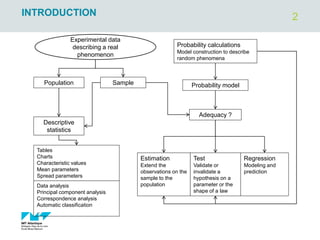
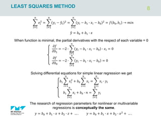
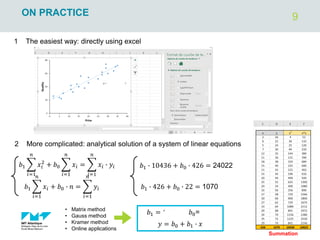
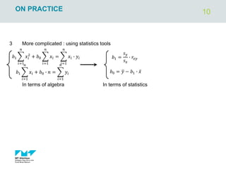
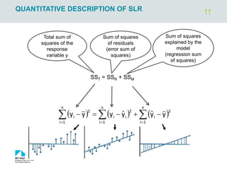
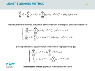
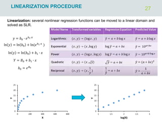
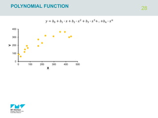
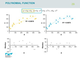
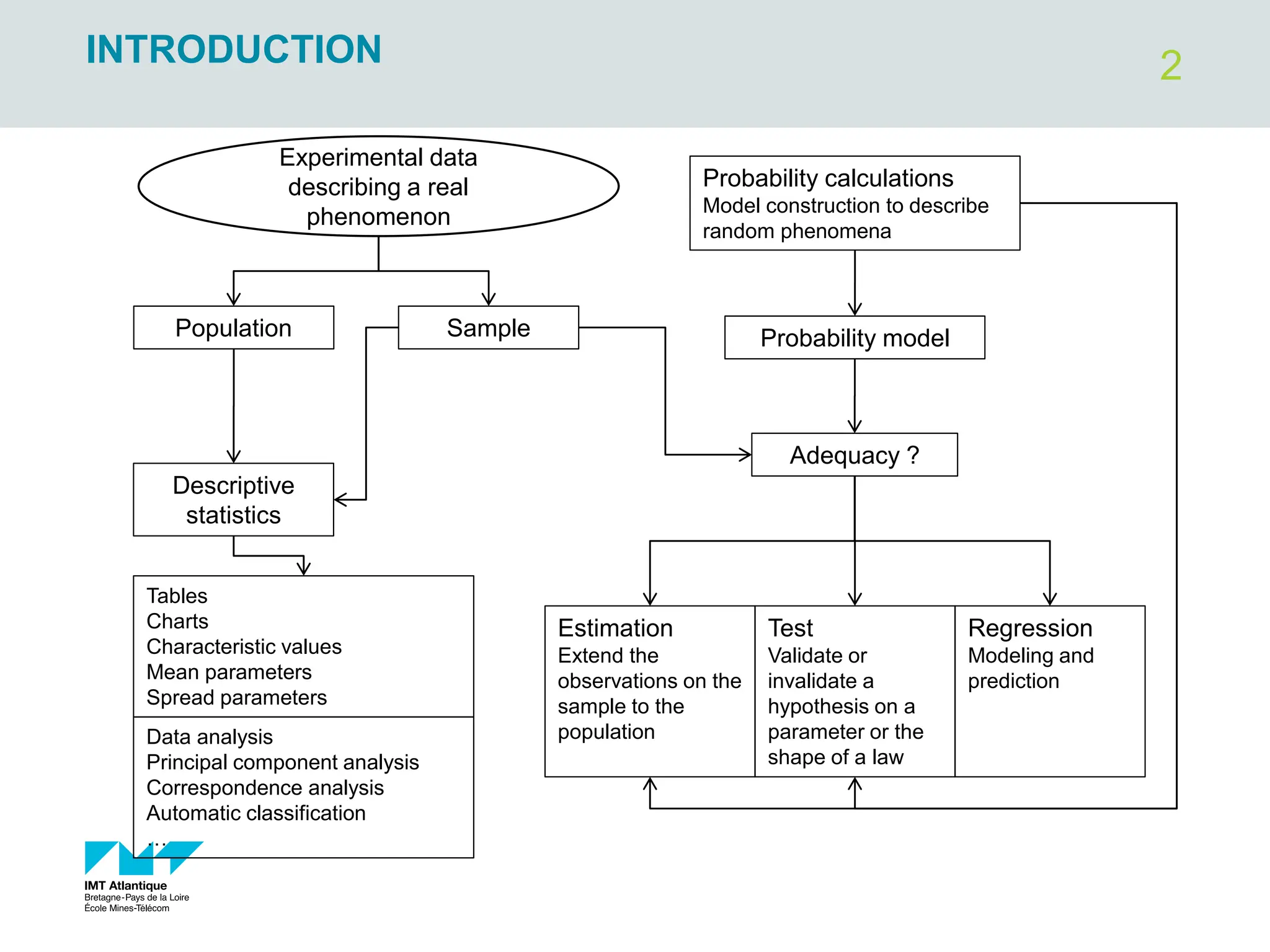
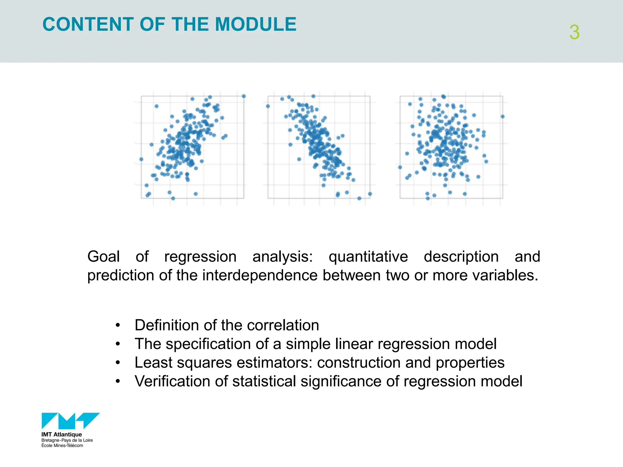
The document outlines regression analysis principles, including correlation and regression modeling, focusing on quantitative description and prediction of variable interdependence. It discusses methods like least squares for determining optimal regression parameters and the importance of statistical diagnostics for validating models. Additionally, it covers practical applications and examples related to linear and nonlinear regression, including confidence intervals and hypothesis testing.

![4
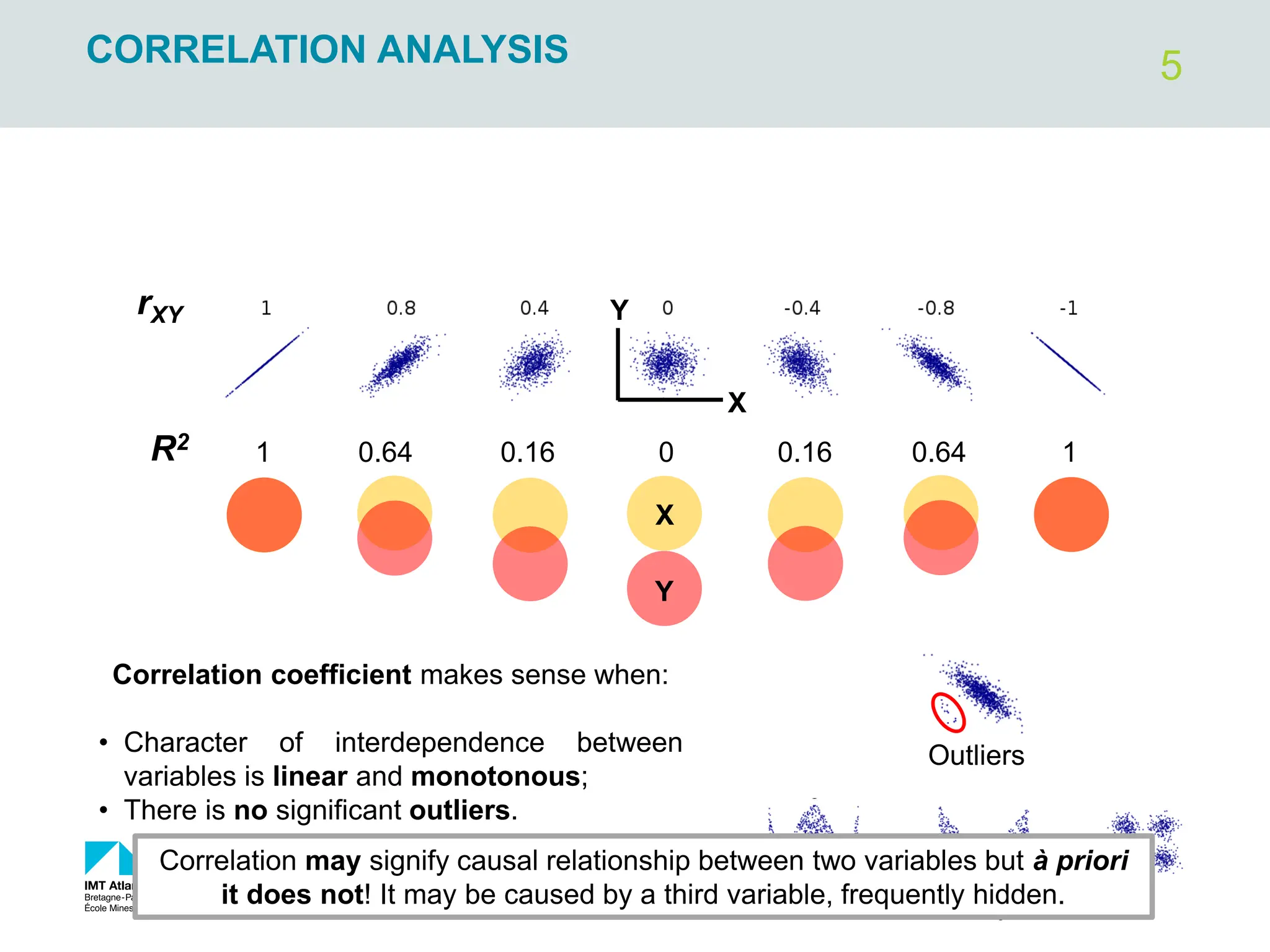
CORRELATION ANALYSIS
X
Y
X
_
Y
_
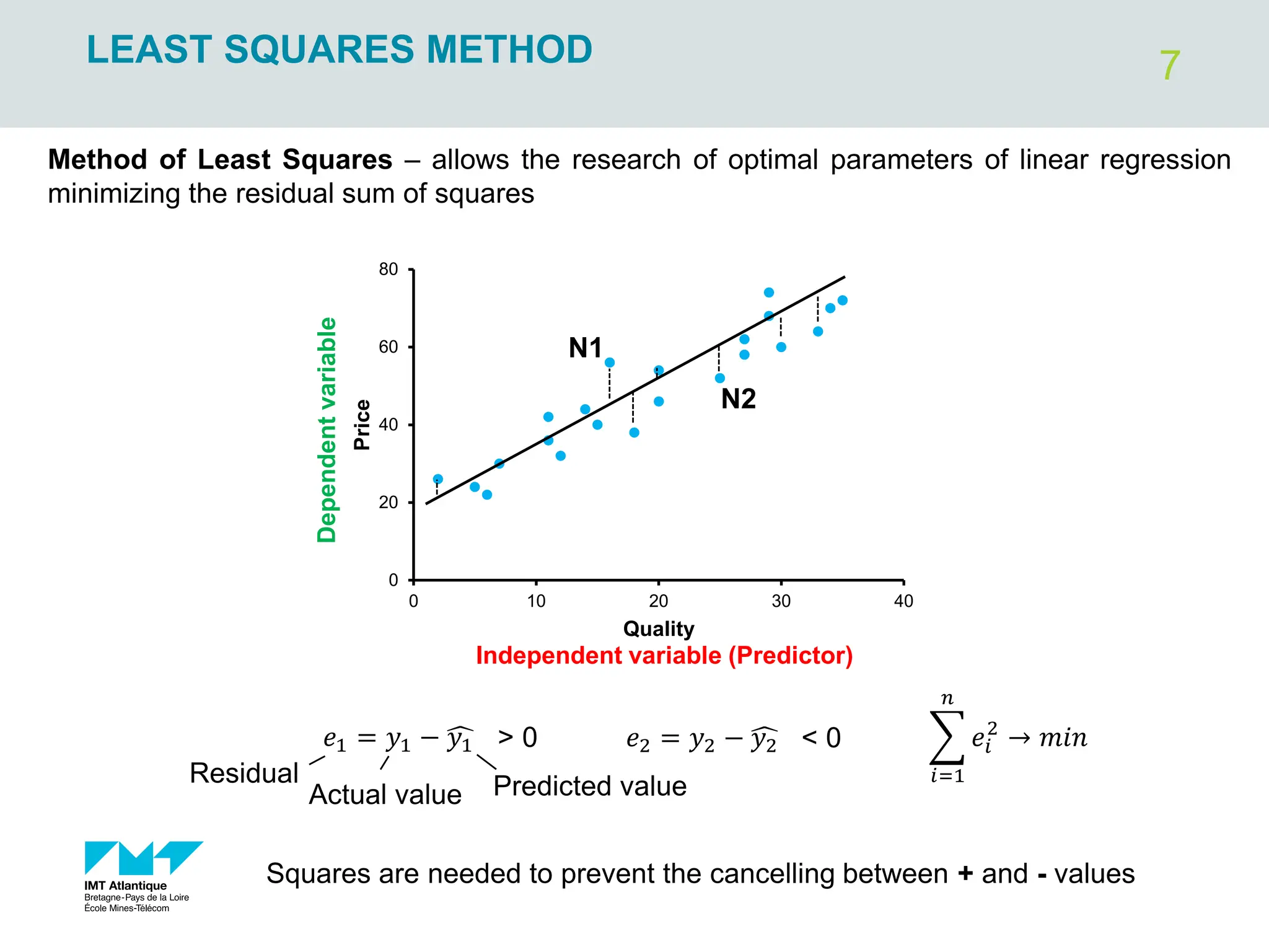
N1
N2
+
+
-
-
X
_
Y
_
Mean height and weight within the
sample
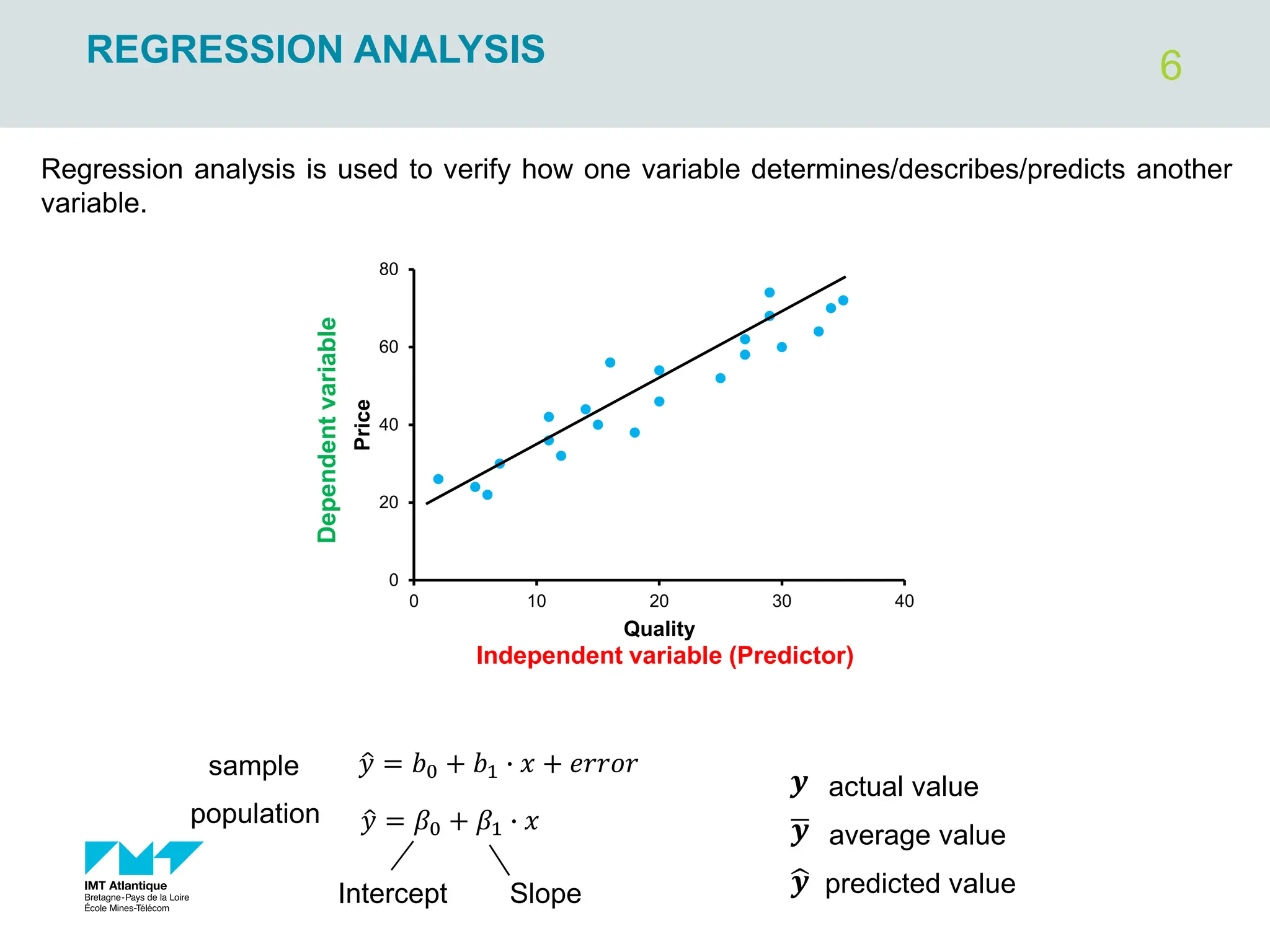
X : Independent or explanatory or exogenous variable
Y: Dependent or response or endogenous variable
Product of deviations from an average
>0 for most of points in case of
positive correlation between X and Y
𝑋1 − ത
𝑋 ∙ 𝑌1 − ത
𝑌 >0
𝑋2 − ത
𝑋 ∙ 𝑌2 − ത
𝑌 >0
𝑋𝑖 − ത
𝑋 ∙ 𝑌𝑖 − ത
𝑌
.
.
.
𝑐𝑜𝑣 =
σ 𝑋𝑖 − ത
𝑋 ∙ 𝑌𝑖 − ത
𝑌
𝑁 − 1
Covariance – quantitatively describes
the strength and the sense of
correlation between variables X and Y
𝑟𝑋𝑌 =
𝑐𝑜𝑣
𝜎𝑋 ∙ 𝜎𝑌
Correlation coefficient (Pearson’s
coefficient) – the same meaning as
covariance but independent on raw
data magnitude. Range: [-1; +1].
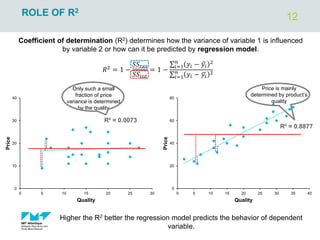
Coefficient of determination 𝑟𝑋𝑌
2
(shared variance) – determine how
the variance of variable 1 is influenced
by variable 2. Range: [0; 1].](https://image.slidesharecdn.com/simplelinearregression2022-240305024922-d5c9bf8c/85/simple-linear-regression-brief-introduction-4-320.jpg)


![4
CORRELATION ANALYSIS
X
Y
X
_
Y
_
N1
N2
+
+
-
-
X
_
Y
_
Mean height and weight within the
sample
X : Independent or explanatory or exogenous variable
Y: Dependent or response or endogenous variable
Product of deviations from an average
>0 for most of points in case of
positive correlation between X and Y
𝑋1 − ത
𝑋 ∙ 𝑌1 − ത
𝑌 >0
𝑋2 − ത
𝑋 ∙ 𝑌2 − ത
𝑌 >0
𝑋𝑖 − ത
𝑋 ∙ 𝑌𝑖 − ത
𝑌
.
.
.
𝑐𝑜𝑣 =
σ 𝑋𝑖 − ത
𝑋 ∙ 𝑌𝑖 − ത
𝑌
𝑁 − 1
Covariance – quantitatively describes
the strength and the sense of
correlation between variables X and Y
𝑟𝑋𝑌 =
𝑐𝑜𝑣
𝜎𝑋 ∙ 𝜎𝑌
Correlation coefficient (Pearson’s
coefficient) – the same meaning as
covariance but independent on raw
data magnitude. Range: [-1; +1].
Coefficient of determination 𝑟𝑋𝑌
2
(shared variance) – determine how
the variance of variable 1 is influenced
by variable 2. Range: [0; 1].](https://image.slidesharecdn.com/simplelinearregression2022-240305024922-d5c9bf8c/75/simple-linear-regression-brief-introduction-4-2048.jpg)