Downloaded 42 times


![R Basics
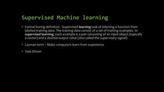
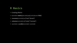
• Assignment :
babu<- c(3,5,7,9)
• Accessing variables:
babu[1] - > 3
• Data types: list, double,character,integer
String example : b <- c("hello","there")
Logiical: a = TRUE
Converting character to integer = factor
• Getting the current directory: getwd()
• tree <-
read.csv(file="trees91.csv",header=TRUE,
sep=",");
names(tree); summary(tree); tree[1]; tree$C
• Listing all variables: ls()
• Type of variables:
typeof(babu)
typeof(list)
• Arithmetic functions: mean(babu)
• Converting array into table: table()](https://image.slidesharecdn.com/supervised-machine-learning-170814061644/85/Supervised-Machine-Learning-in-R-7-320.jpg)

![Input Data
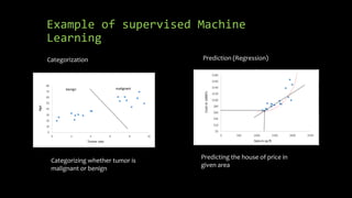
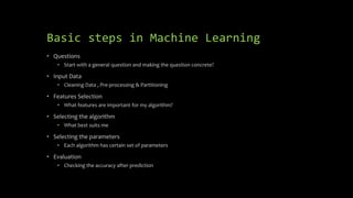
• Cleaning
• input<- read.csv("pml-training.csv", na.strings = c("NA", "#DIV/0!", ""))
• input =input[,colSums(is.na(input)) == 0]
• standardization
standardhousing <-(housing$Home.Value-
mean(housing$Home.Value))/(sd(housing$Home.Value))
• Removing Near Zero covariates
nsvCol =nearZeroVar(housing)](https://image.slidesharecdn.com/supervised-machine-learning-170814061644/85/Supervised-Machine-Learning-in-R-11-320.jpg)
![Input Data
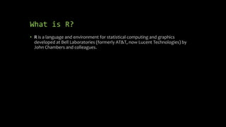
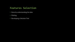
• Partitioning the Data is done early
• Thumbs of Rule of partitioning
• 40% -testing, 60% - training or 70% -training 30% -testing for medium data sets
• 20%-testing, 20%-validation, 60%- validation
• R Code for partitioning:
• library(caret)
• set.seed(11051985)
• inTrain <- createDataPartition(y=input$classe, p=0.70, list=FALSE)
• training <- input[inTrain,]
• testing <- input[-inTrain,]](https://image.slidesharecdn.com/supervised-machine-learning-170814061644/85/Supervised-Machine-Learning-in-R-12-320.jpg)

![Calculating Accuracy
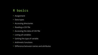
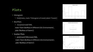
• confMatrix<- confusionMatrix(predictions, testing$Survived)
## Confusion Matrix and Statistics
##
## Reference
## Prediction 0 1
## 0 506 88
## 1 43 254
##
## Accuracy : 0.853
## 95% CI : (0.828, 0.8756)
## No Information Rate : 0.6162
## P-Value [Acc > NIR] : < 2.2e-16
##
## Kappa : 0.6813
## Mcnemar's Test P-Value : 0.0001209
##
## Sensitivity : 0.9217
## Specificity : 0.7427
## Pos Pred Value : 0.8519
## Neg Pred Value : 0.8552
## Prevalence : 0.6162
## Detection Rate : 0.5679
## Detection Prevalence : 0.6667
## Balanced Accuracy : 0.8322
##
## 'Positive' Class : 0](https://image.slidesharecdn.com/supervised-machine-learning-170814061644/85/Supervised-Machine-Learning-in-R-26-320.jpg)


![R Basics
• Assignment :
babu<- c(3,5,7,9)
• Accessing variables:
babu[1] - > 3
• Data types: list, double,character,integer
String example : b <- c("hello","there")
Logiical: a = TRUE
Converting character to integer = factor
• Getting the current directory: getwd()
• tree <-
read.csv(file="trees91.csv",header=TRUE,
sep=",");
names(tree); summary(tree); tree[1]; tree$C
• Listing all variables: ls()
• Type of variables:
typeof(babu)
typeof(list)
• Arithmetic functions: mean(babu)
• Converting array into table: table()](https://image.slidesharecdn.com/supervised-machine-learning-170814061644/75/Supervised-Machine-Learning-in-R-7-2048.jpg)

![Input Data
• Cleaning
• input<- read.csv("pml-training.csv", na.strings = c("NA", "#DIV/0!", ""))
• input =input[,colSums(is.na(input)) == 0]
• standardization
standardhousing <-(housing$Home.Value-
mean(housing$Home.Value))/(sd(housing$Home.Value))
• Removing Near Zero covariates
nsvCol =nearZeroVar(housing)](https://image.slidesharecdn.com/supervised-machine-learning-170814061644/75/Supervised-Machine-Learning-in-R-11-2048.jpg)
![Input Data
• Partitioning the Data is done early
• Thumbs of Rule of partitioning
• 40% -testing, 60% - training or 70% -training 30% -testing for medium data sets
• 20%-testing, 20%-validation, 60%- validation
• R Code for partitioning:
• library(caret)
• set.seed(11051985)
• inTrain <- createDataPartition(y=input$classe, p=0.70, list=FALSE)
• training <- input[inTrain,]
• testing <- input[-inTrain,]](https://image.slidesharecdn.com/supervised-machine-learning-170814061644/75/Supervised-Machine-Learning-in-R-12-2048.jpg)

![Calculating Accuracy
• confMatrix<- confusionMatrix(predictions, testing$Survived)
## Confusion Matrix and Statistics
##
## Reference
## Prediction 0 1
## 0 506 88
## 1 43 254
##
## Accuracy : 0.853
## 95% CI : (0.828, 0.8756)
## No Information Rate : 0.6162
## P-Value [Acc > NIR] : < 2.2e-16
##
## Kappa : 0.6813
## Mcnemar's Test P-Value : 0.0001209
##
## Sensitivity : 0.9217
## Specificity : 0.7427
## Pos Pred Value : 0.8519
## Neg Pred Value : 0.8552
## Prevalence : 0.6162
## Detection Rate : 0.5679
## Detection Prevalence : 0.6667
## Balanced Accuracy : 0.8322
##
## 'Positive' Class : 0](https://image.slidesharecdn.com/supervised-machine-learning-170814061644/75/Supervised-Machine-Learning-in-R-26-2048.jpg)


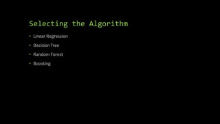
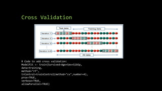
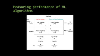
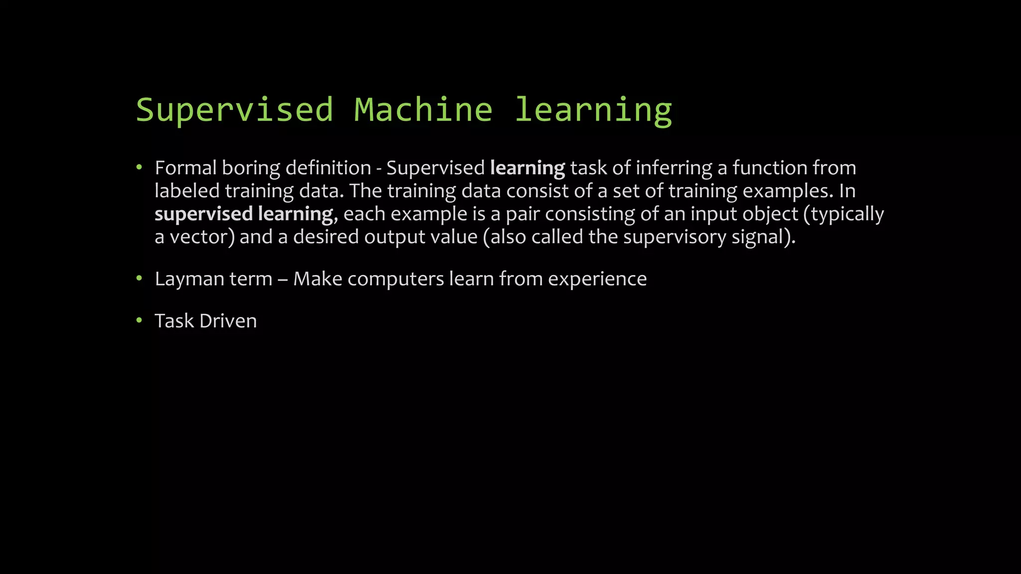
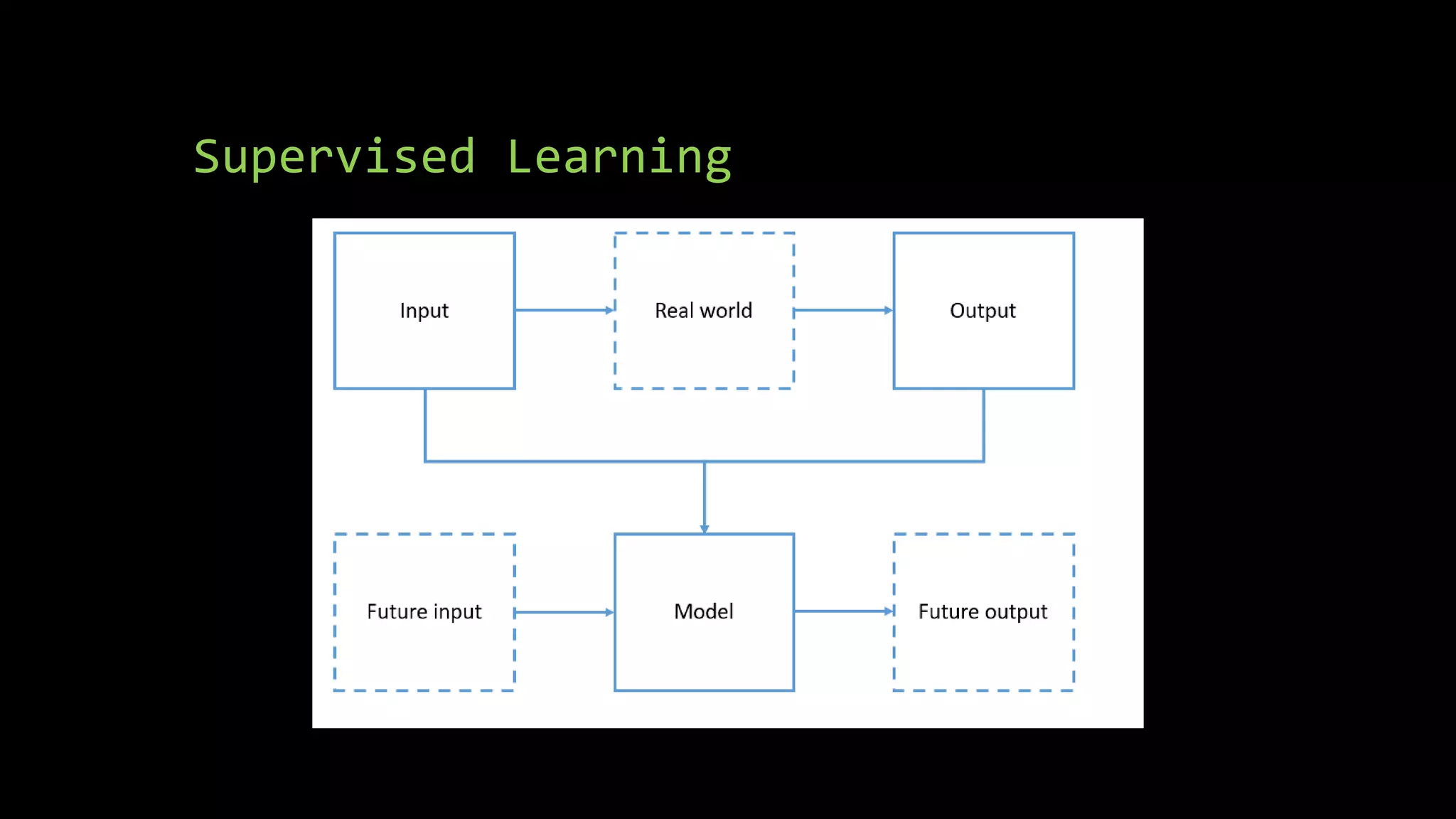
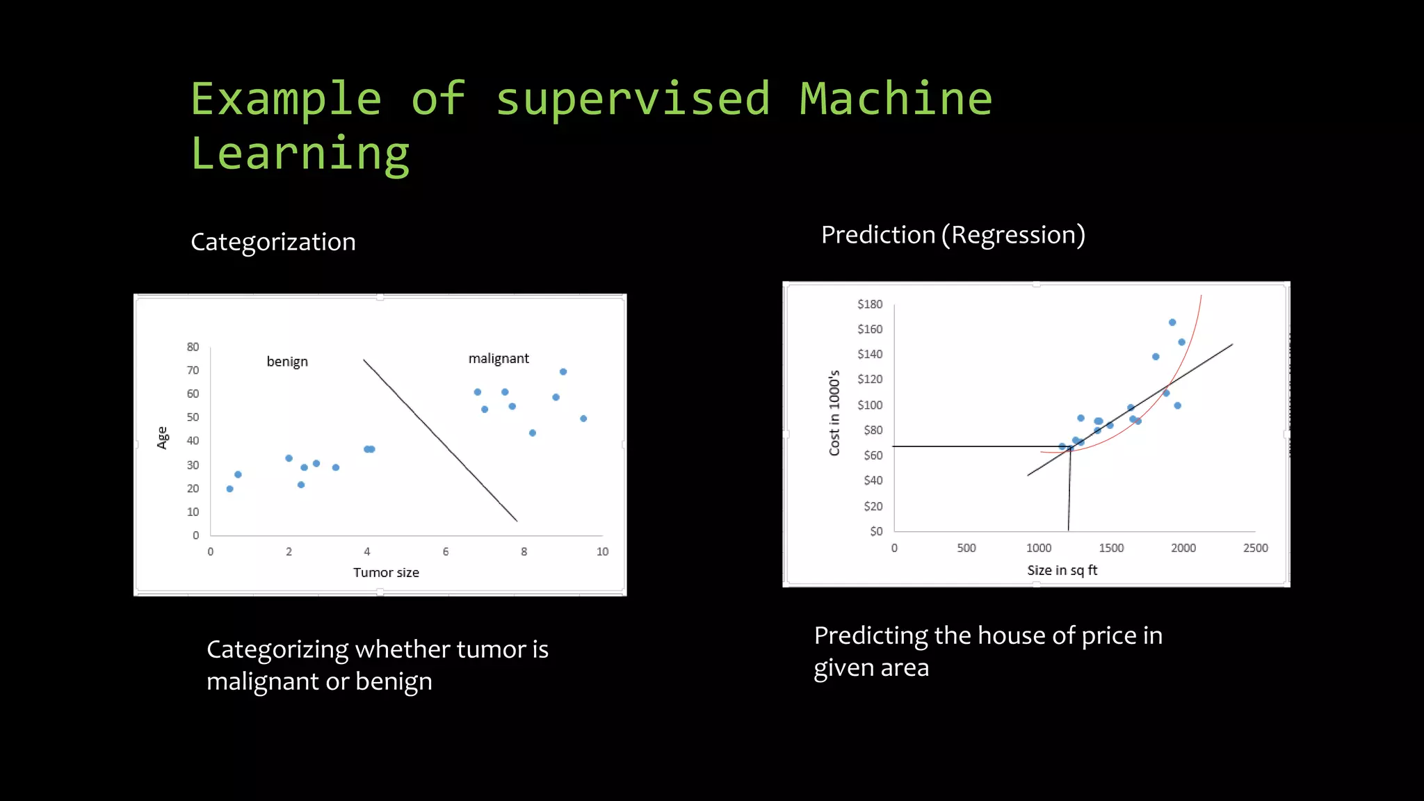
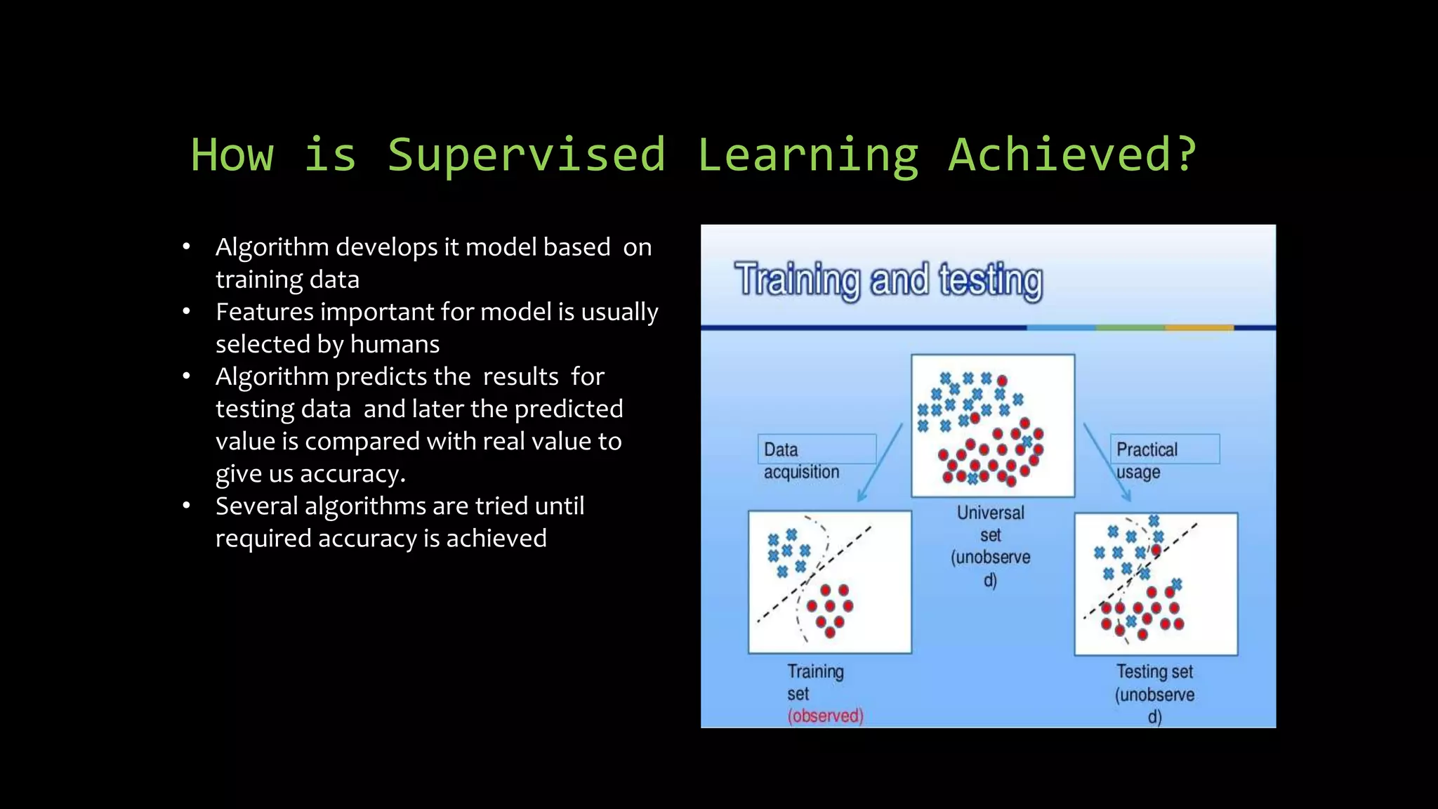
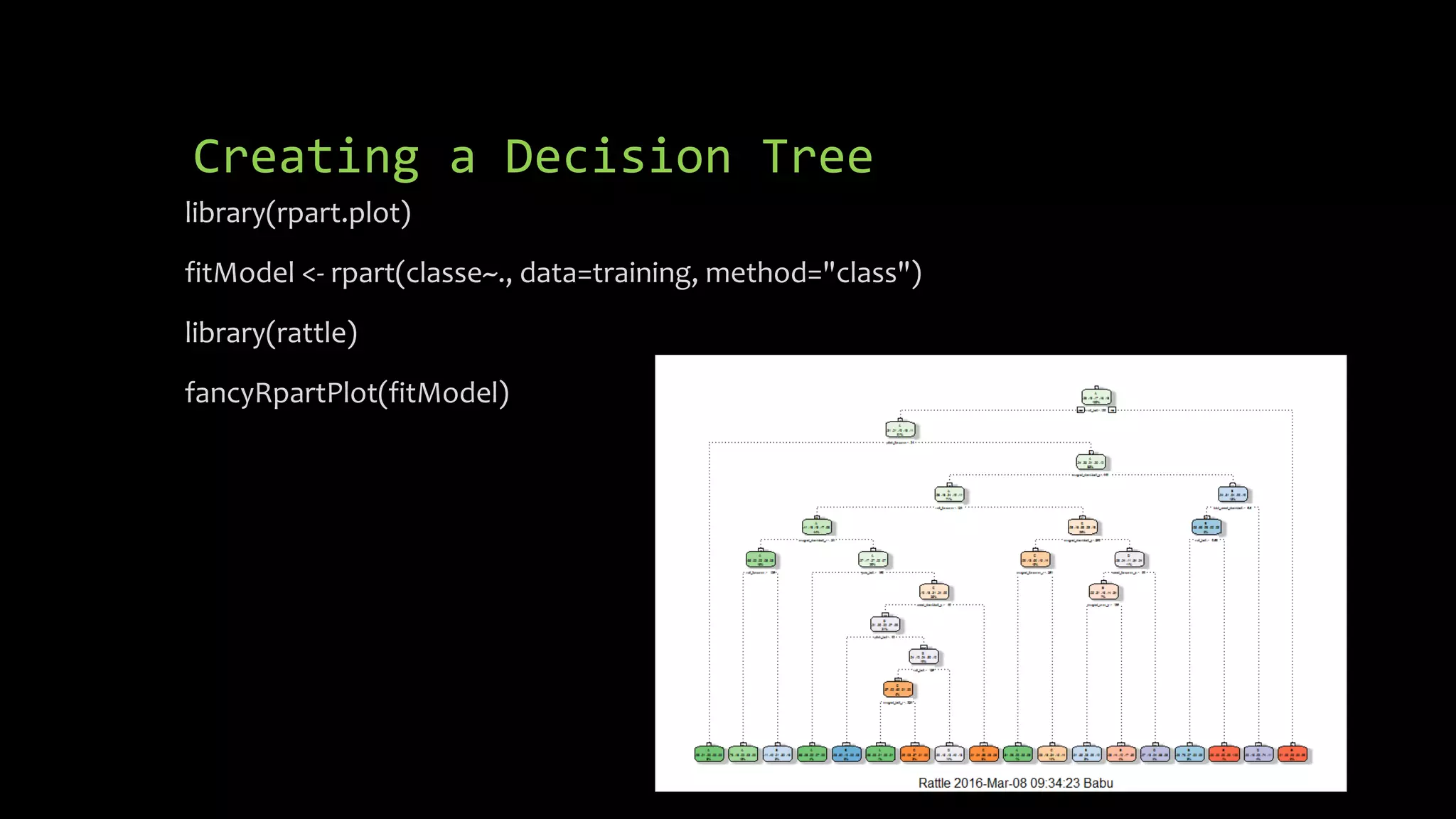
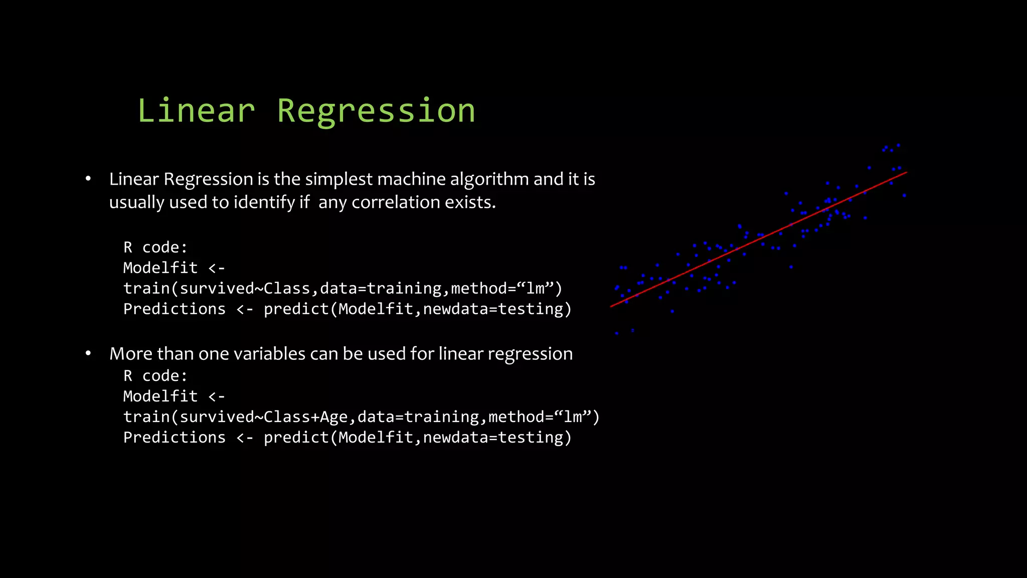
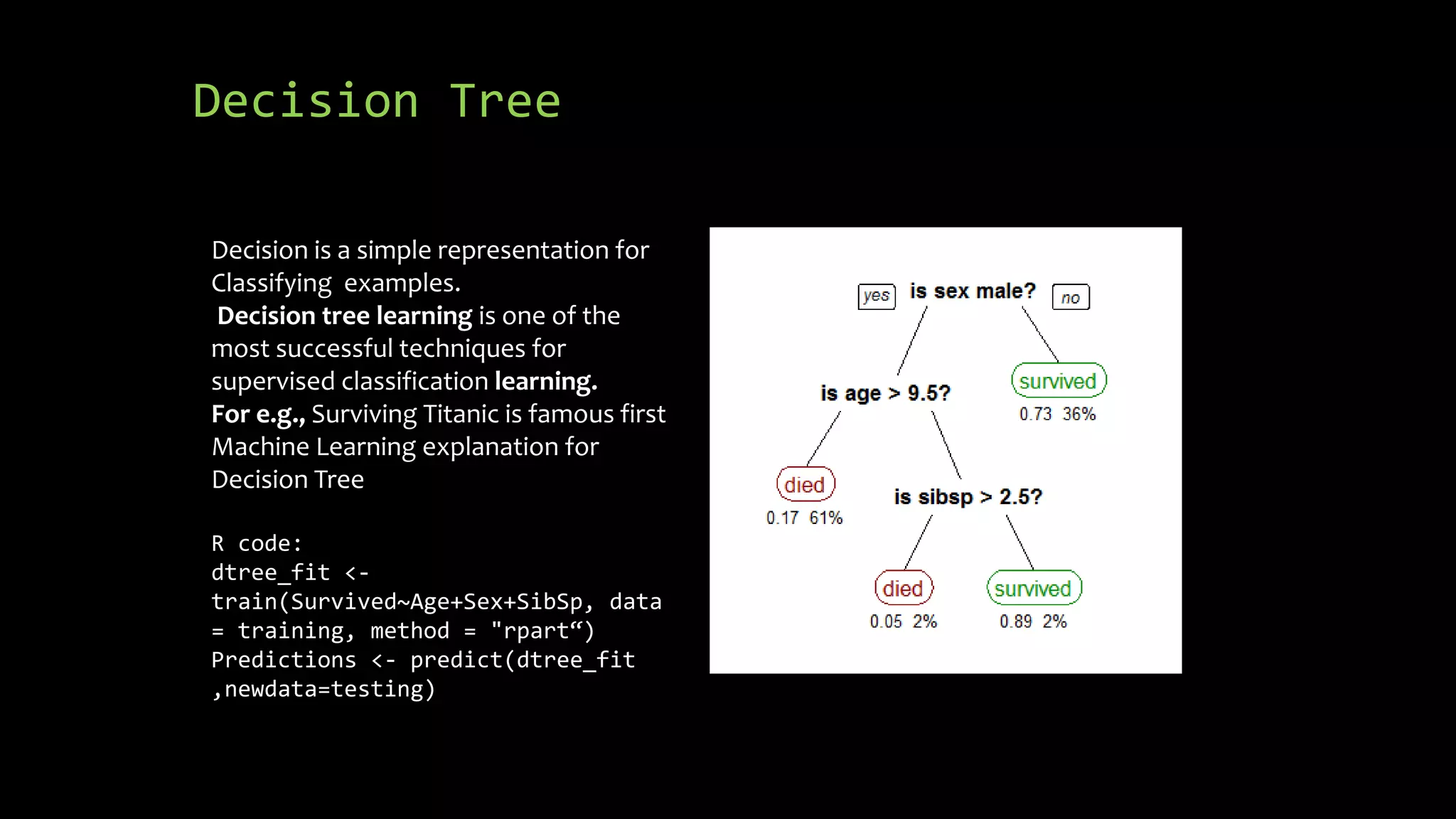
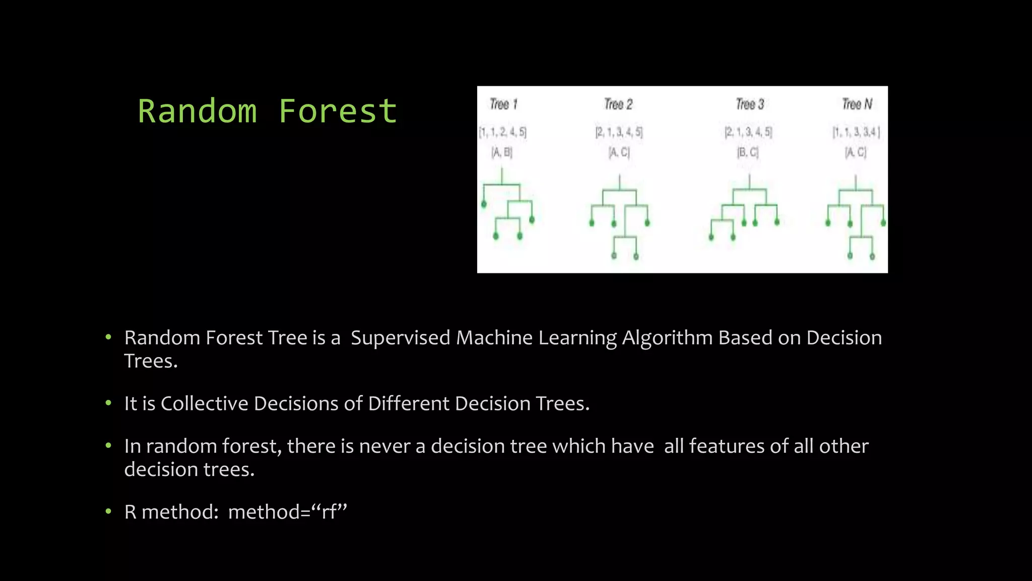
The document discusses supervised machine learning using R, explaining its definition, basic operations, and algorithms including linear regression, decision trees, and random forests. It outlines data preparation steps like cleaning, partitioning, and feature selection, along with providing R code examples for various tasks. Additionally, it highlights the performance evaluation of machine learning models using confusion matrices and accuracy metrics.


