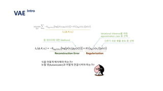
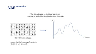
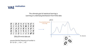
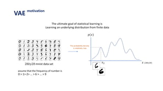
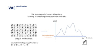
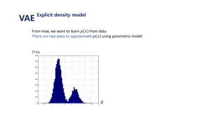
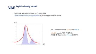
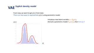
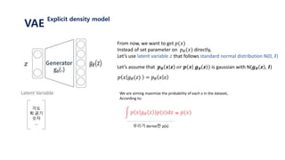
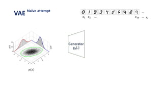
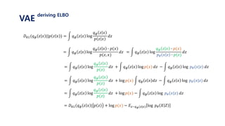
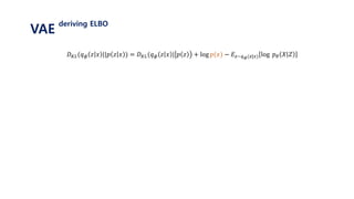
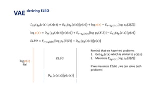
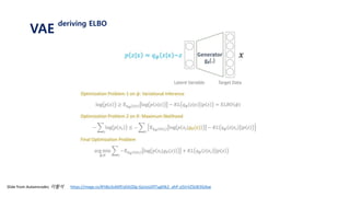
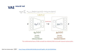
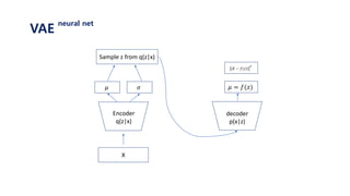
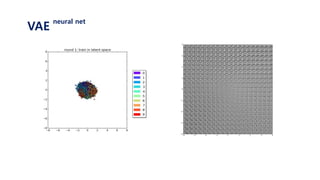
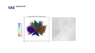
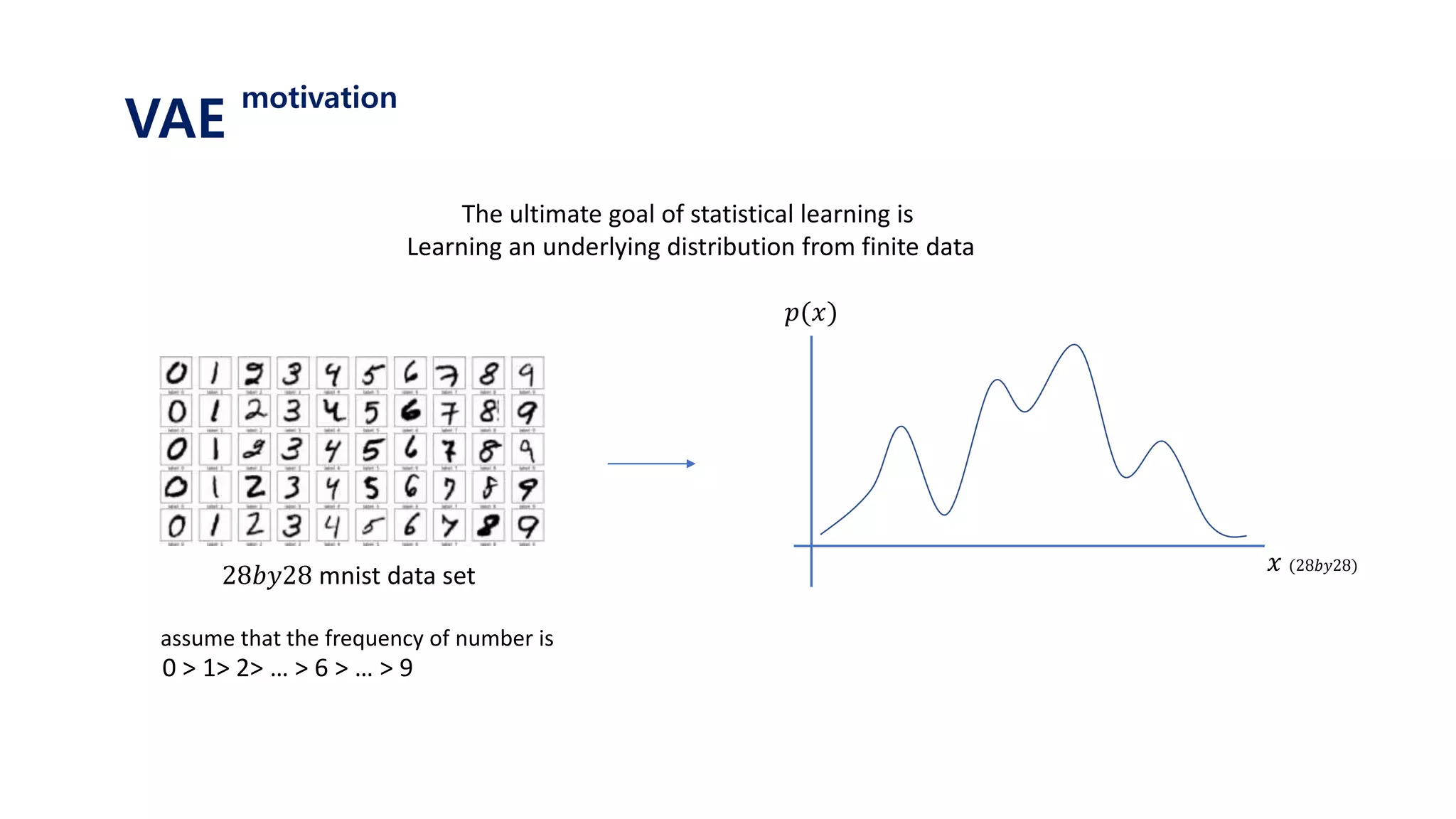
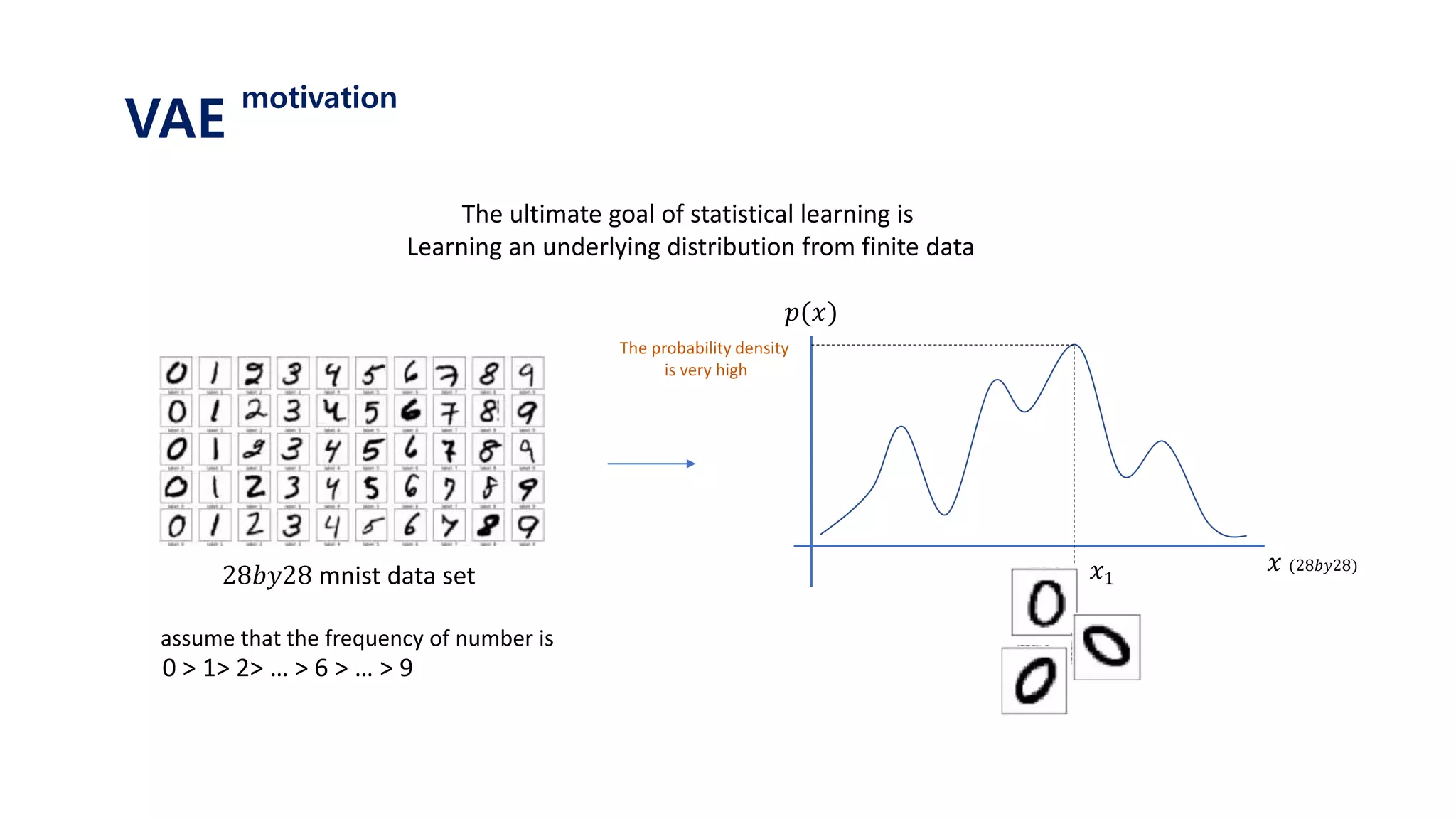
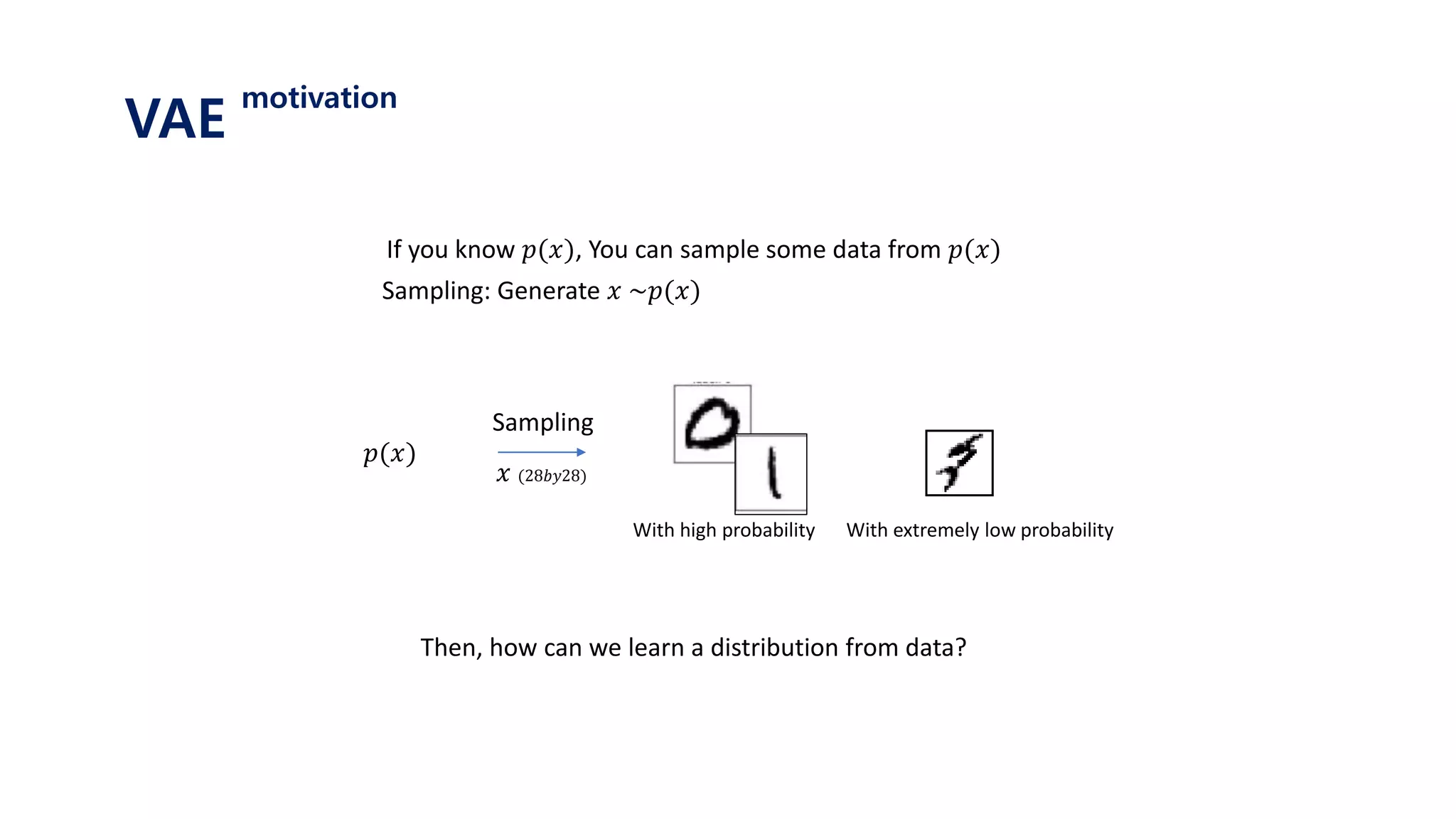
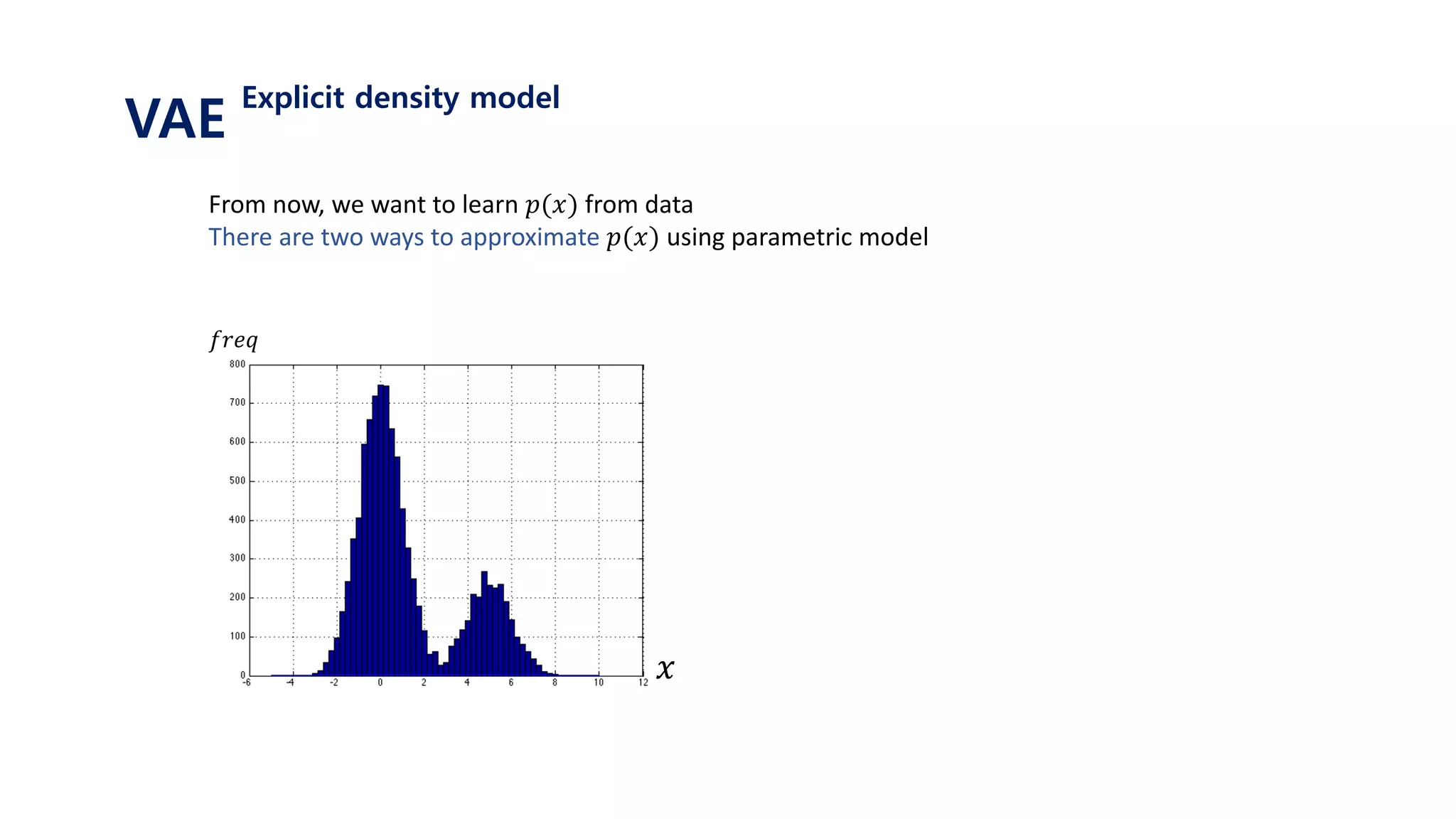
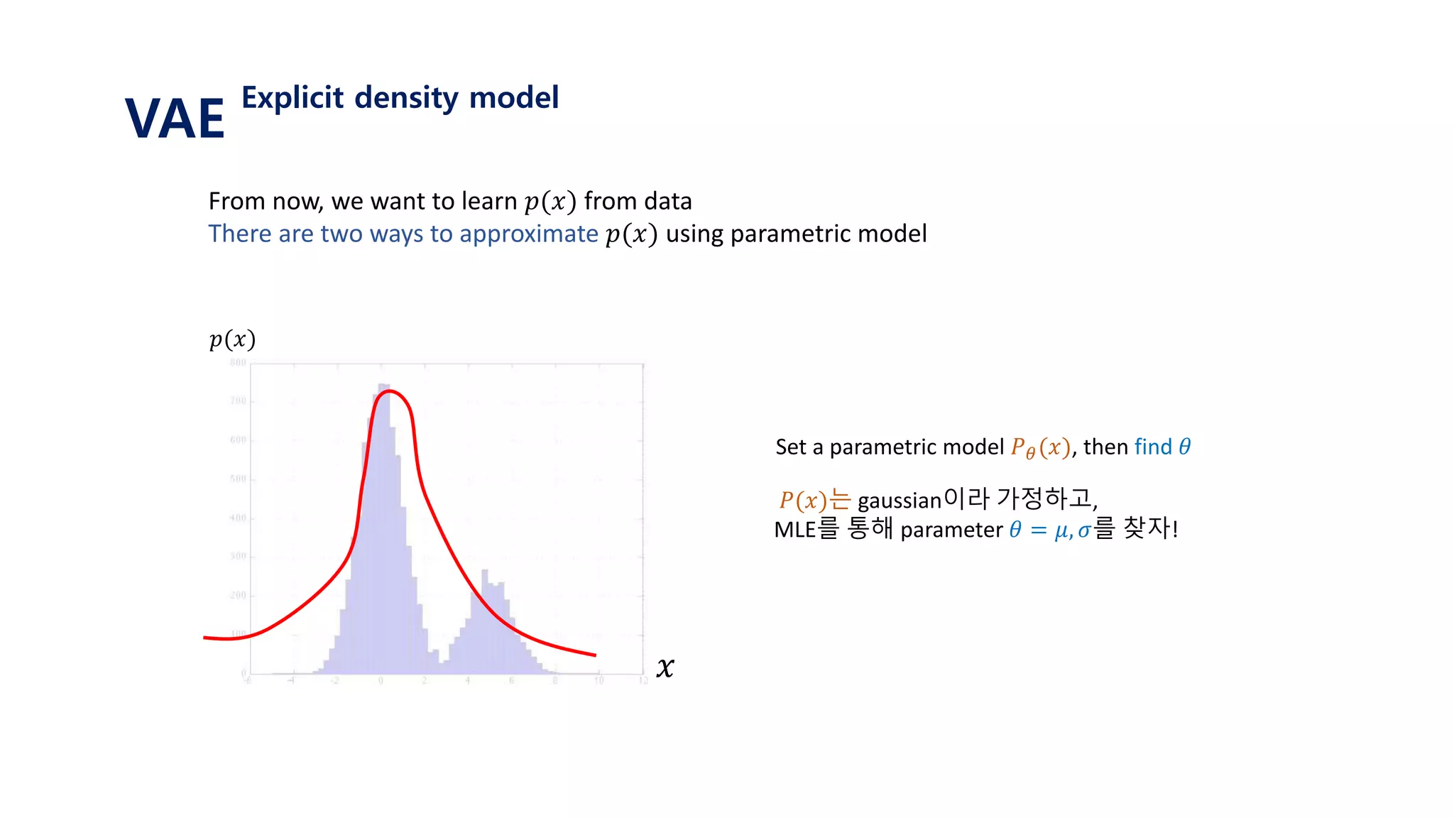
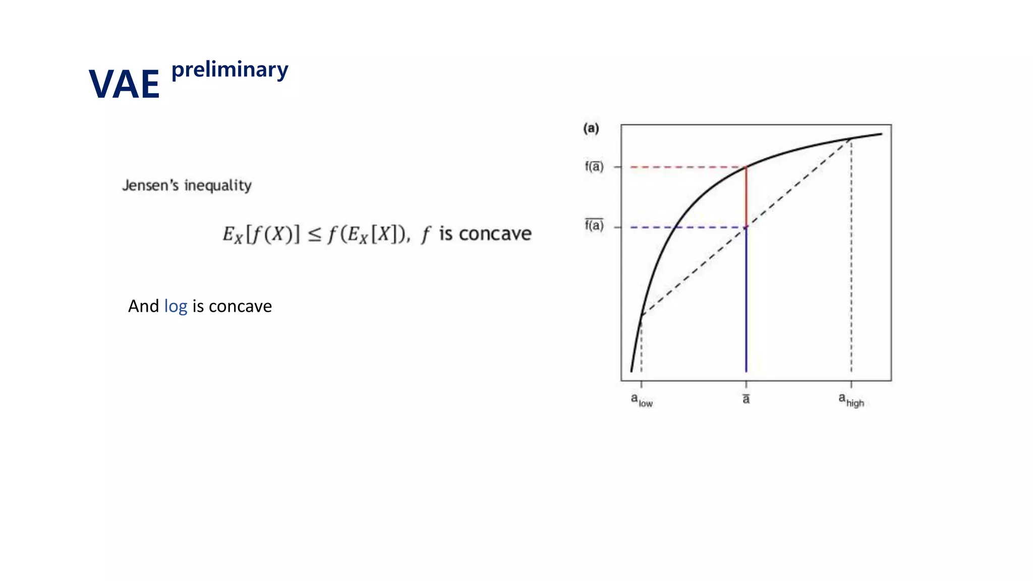
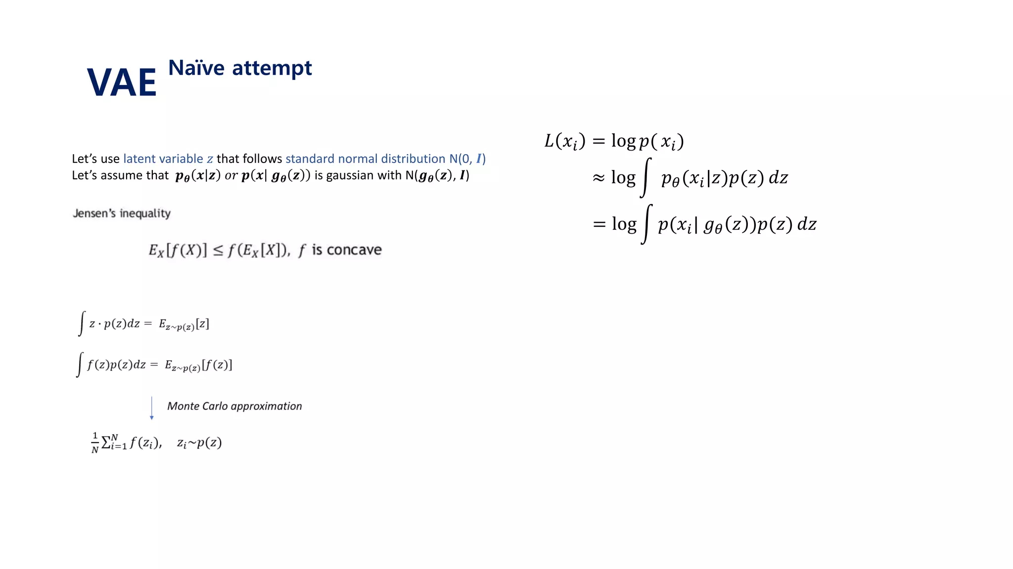
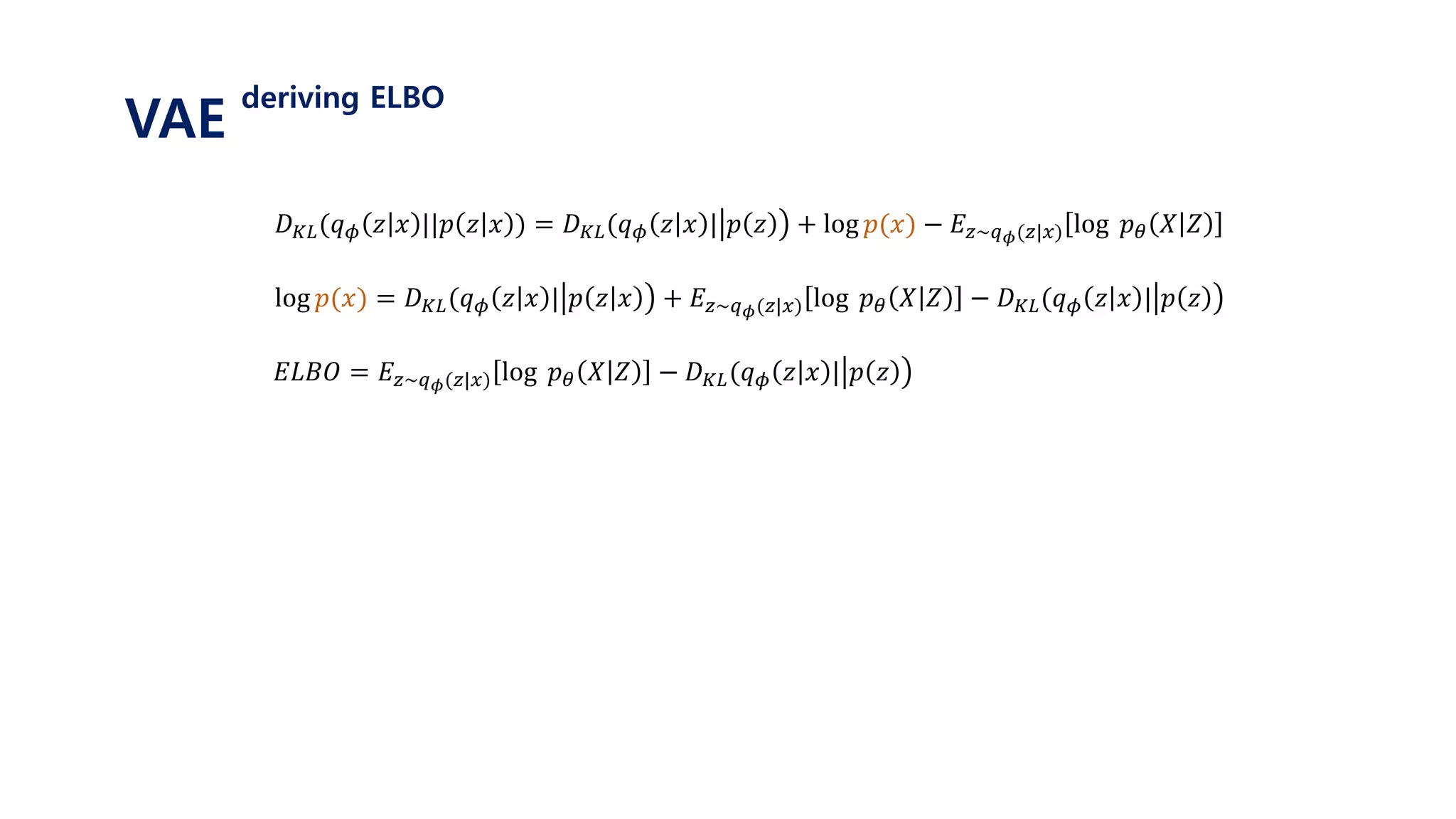
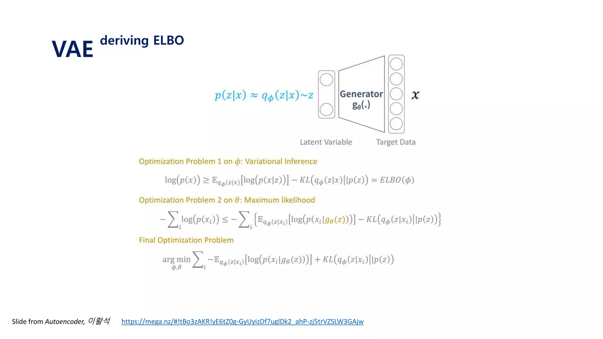
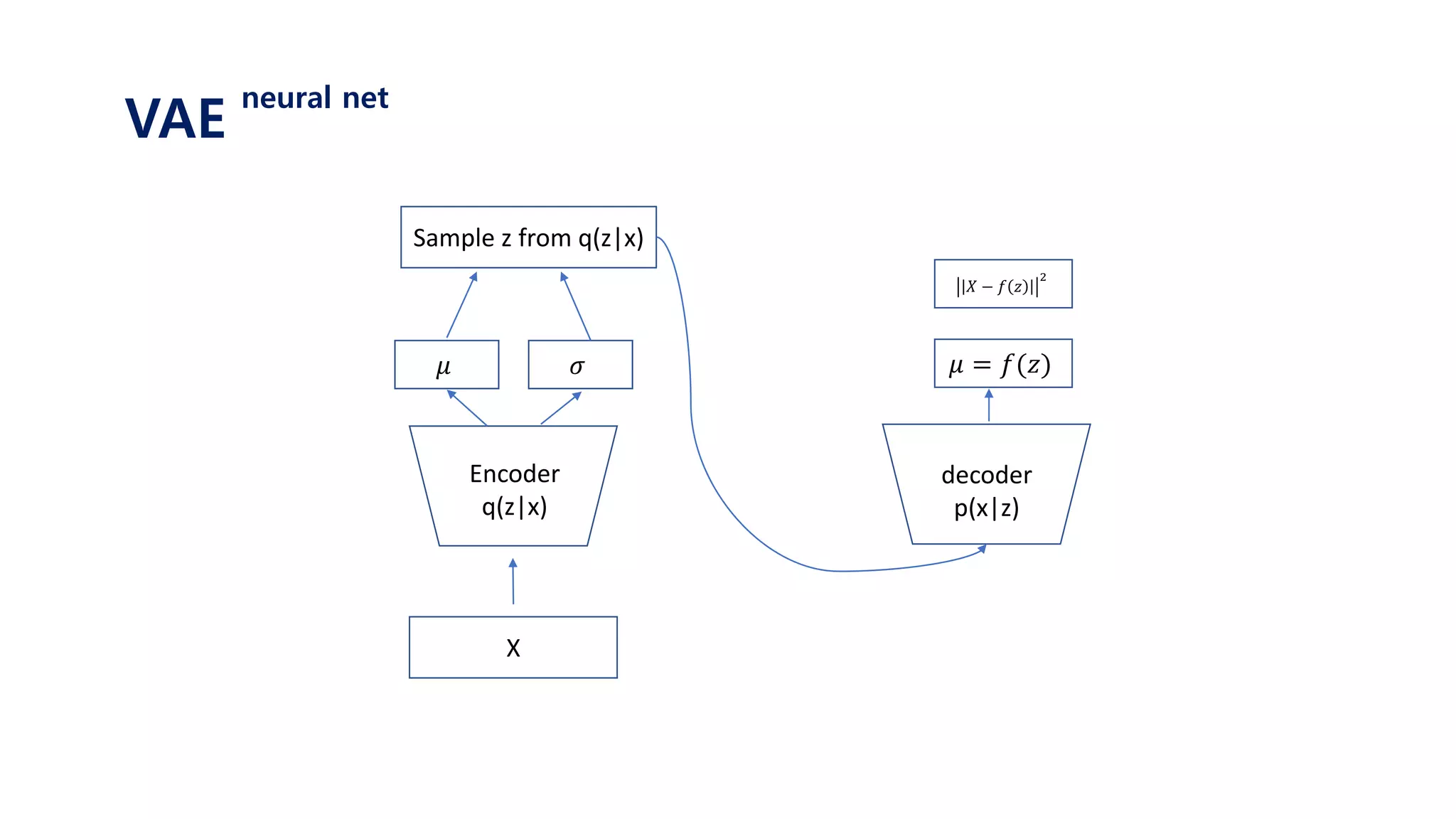
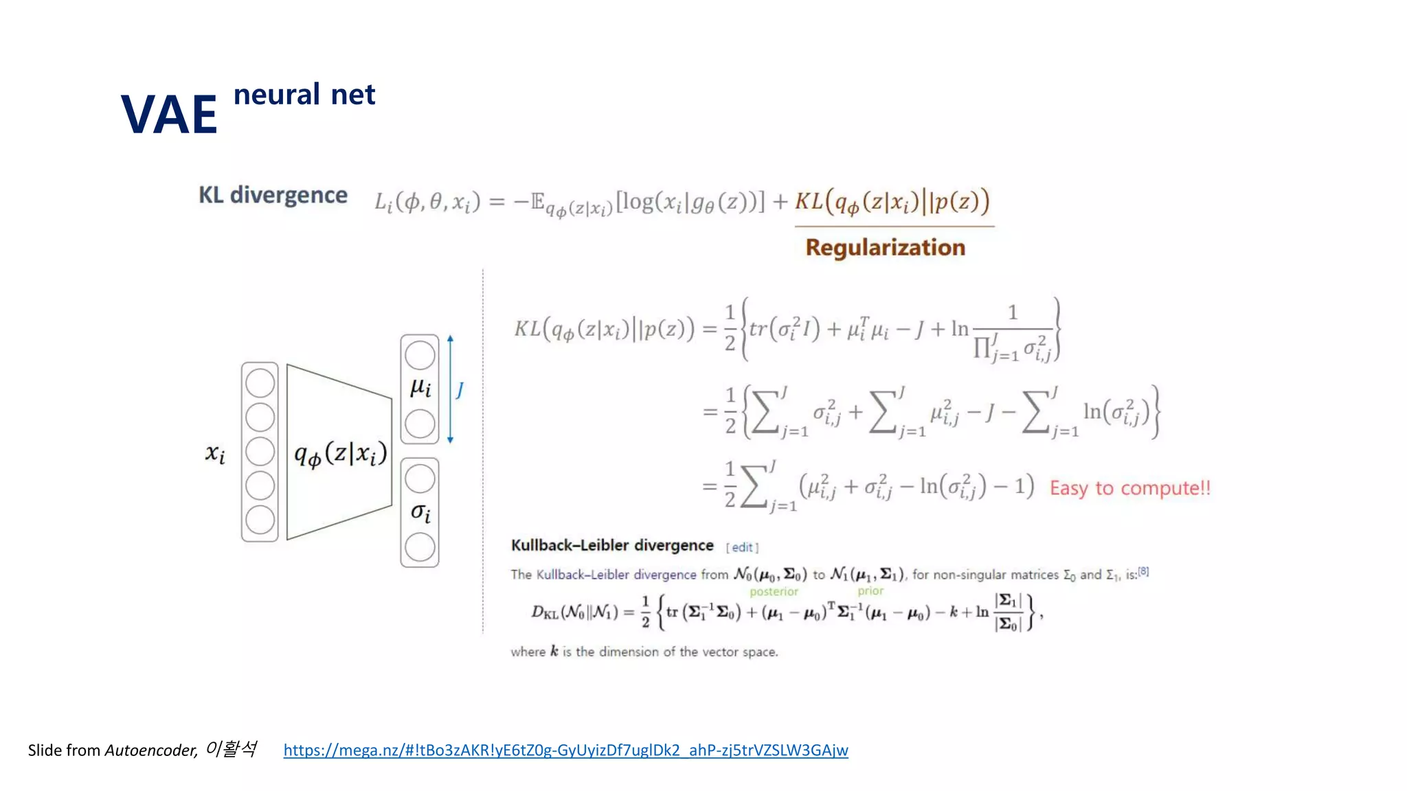
The document provides an introduction to variational autoencoders (VAE). It discusses how VAEs can be used to learn the underlying distribution of data by introducing a latent variable z that follows a prior distribution like a standard normal. The document outlines two approaches - explicitly modeling the data distribution p(x), or using the latent variable z. It suggests using z and assuming the conditional distribution p(x|z) is a Gaussian with mean determined by a neural network gθ(z). The goal is to maximize the likelihood of the dataset by optimizing the evidence lower bound objective.

![𝐿 𝑊, 𝑏, 𝑊, 𝑏 =
𝑛=1
𝑁
𝑥 𝑛 − 𝑥 𝑥 𝑛
2
If the shape of W is [n,m],
than the shape of 𝑊 is [m,n]
𝑦𝑛
Generally, 𝑊 is not 𝑊 𝑇,
but weight sharing is also possible!
(to reduce the number of parameters)
𝑦1
Autoencoder](https://image.slidesharecdn.com/180208tutorialonvaelabseminar-180720033633/85/Variational-Autoencoder-Tutorial-4-320.jpg)

![input
𝑥
output
𝑓𝜃(𝑥)
data parameter
𝑦𝑓𝜃1 𝑥
𝑝(𝑦| 𝑓𝜃1 𝑥 )𝑚𝑎𝑥𝑖𝑚𝑖𝑧𝑒 𝒑 𝜽 𝒚 𝒙 𝑜𝑟 𝒑 𝒚 𝒇 𝜽 𝒙
𝑚𝑖𝑛𝑖𝑚𝑖𝑧𝑒 − 𝐥𝐨𝐠[𝒑 𝒚 𝒇 𝜽 𝒙 ]
VAE
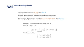
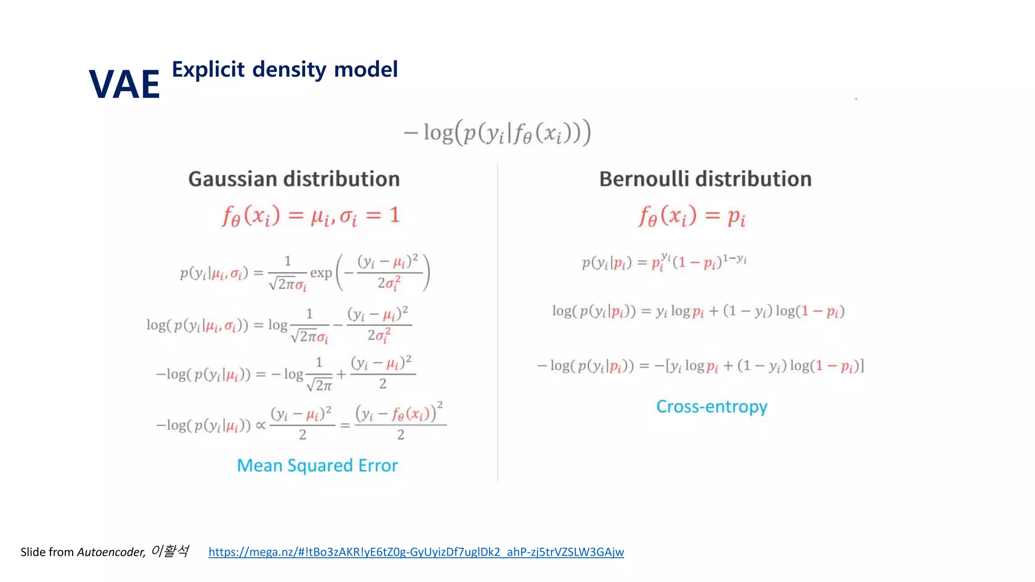
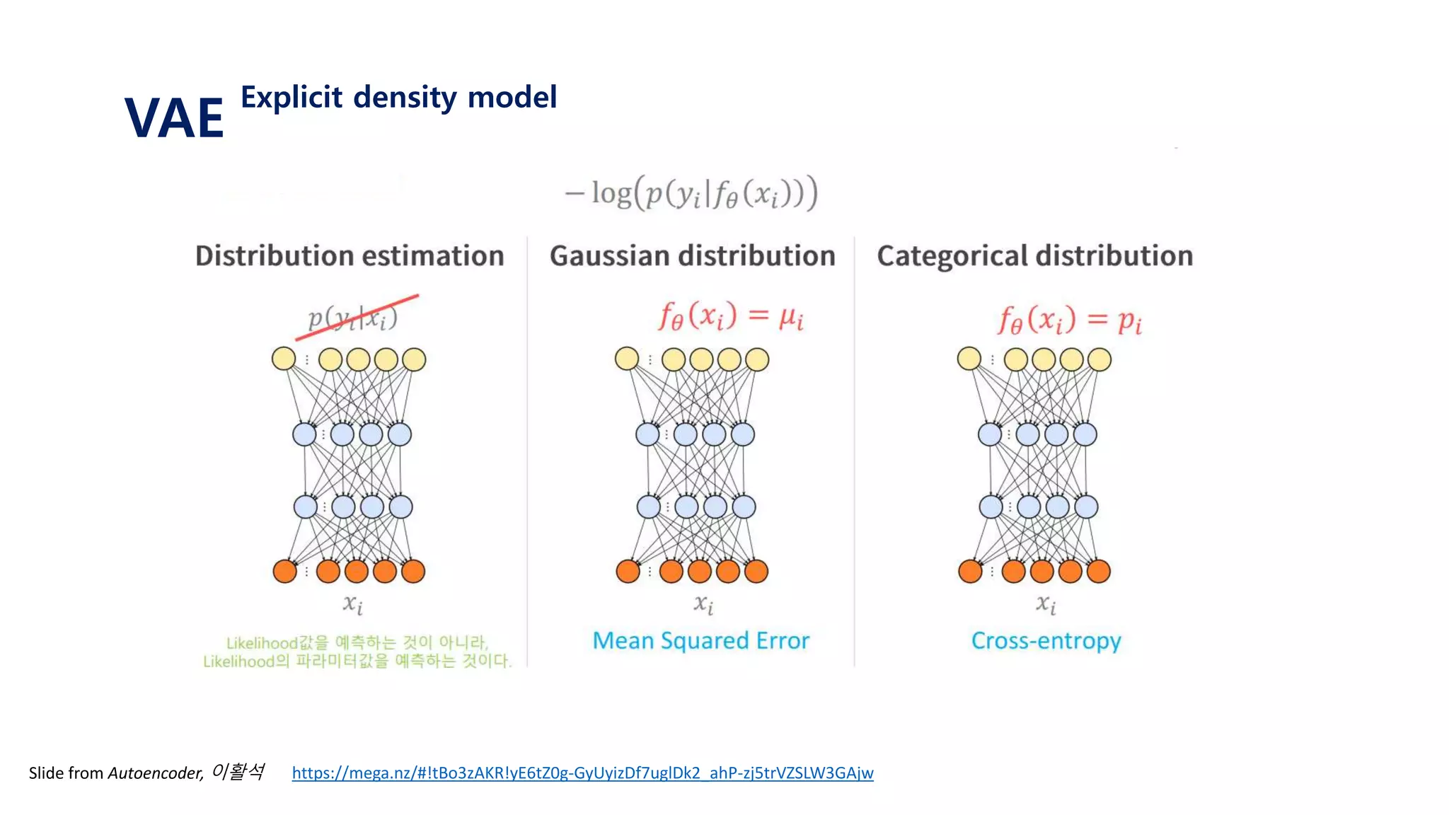
Explicit density model
assume that 𝑝 𝜃 𝑦 𝑥 follows normal distribution, N(𝑓𝜃 𝑥 , 1)
find 𝑓𝜃 𝑥 that maximize 𝑝 𝜃 𝑦 𝑥 using neural net
Actually, we do this using neural Net!
The output of neural net is parameter of distribution
N(𝑓𝜃 𝑥 , 1) 인 정규분포에서 데이터 y가 나올 확률밀도 값을 얻을 수 있음, 𝒑 𝒚 𝒇 𝜽 𝒙
이를 최대화 하는 방향으로 업데이트!](https://image.slidesharecdn.com/180208tutorialonvaelabseminar-180720033633/85/Variational-Autoencoder-Tutorial-14-320.jpg)
![input
𝑥
output
𝑓𝜃(𝑥)
data parameter
𝑦𝑓𝜃1 𝑥
𝑝(𝑦| 𝑓𝜃1 𝑥 ) <
𝑓𝜃2 𝑥
𝑝(𝑦| 𝑓𝜃2 𝑥 )𝑚𝑎𝑥𝑖𝑚𝑖𝑧𝑒 𝒑 𝜽 𝒚 𝒙 𝑜𝑟 𝒑 𝒚 𝒇 𝜽 𝒙
𝑚𝑖𝑛𝑖𝑚𝑖𝑧𝑒 − 𝐥𝐨𝐠[𝒑 𝒚 𝒇 𝜽 𝒙 ]
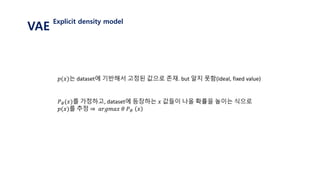
VAE
Explicit density model
assume that 𝑝 𝜃 𝑦 𝑥 follows normal distribution, N(𝑓𝜃 𝑥 , 1)
find 𝑓𝜃 𝑥 that maximize 𝑝 𝜃 𝑦 𝑥 using neural net
Actually, we do this using neural Net!
The output of neural net is parameter of distribution](https://image.slidesharecdn.com/180208tutorialonvaelabseminar-180720033633/85/Variational-Autoencoder-Tutorial-15-320.jpg)
![input
𝑥
output
𝑓𝜃(𝑥)
data parameter
𝑦𝑓𝜃1 𝑥 𝑓𝜃2 𝑥 = 𝑓𝜃3 𝑥
𝑚𝑎𝑥𝑖𝑚𝑖𝑧𝑒 𝒑 𝜽 𝒚 𝒙 𝑜𝑟 𝒑 𝒚 𝒇 𝜽 𝒙
𝑚𝑖𝑛𝑖𝑚𝑖𝑧𝑒 − 𝐥𝐨𝐠[𝒑 𝒚 𝒇 𝜽 𝒙 ]
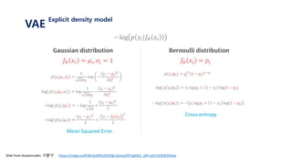
VAE
Explicit density model
assume that 𝑝 𝜃 𝑦 𝑥 follows normal distribution, N(𝑓𝜃 𝑥 , 1)
find 𝑓𝜃 𝑥 that maximize 𝑝 𝜃 𝑦 𝑥 using neural net
Actually, we do this using neural Net!
The output of neural net is parameter of distribution](https://image.slidesharecdn.com/180208tutorialonvaelabseminar-180720033633/85/Variational-Autoencoder-Tutorial-16-320.jpg)
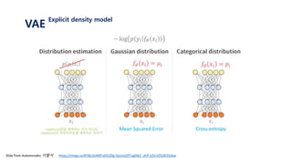


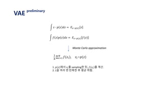

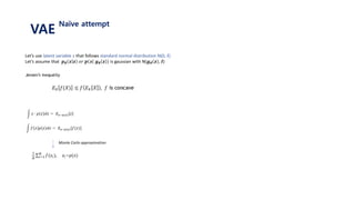
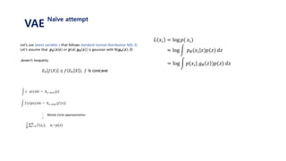
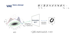
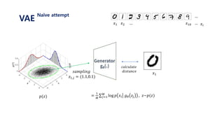
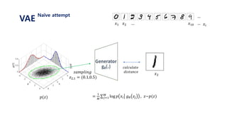
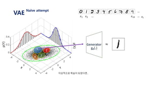
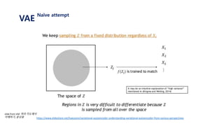
![𝐿 𝑥𝑖 = log 𝑝( 𝑥𝑖)
Let’s use latent variable 𝑧 that follows standard normal distribution N(0, 𝑰)
Let’s assume that 𝒑 𝜽 𝒙 𝒛 𝑜𝑟 𝒑 𝒙 𝒈 𝜽 𝒛 is gaussian with N(𝒈 𝜽 𝒛 , 𝑰) ≈ log 𝑝 𝜃(𝑥𝑖|𝑧)𝑝(𝑧) 𝑑𝑧
= log 𝑝(𝑥𝑖| 𝑔 𝜃 𝑧 )𝑝(𝑧) 𝑑𝑧
= log 𝐸𝑧~𝑝(𝑧)[𝑝 𝑥𝑖 𝑔 𝜃 𝑧 ]
≥ 𝐸𝑧~𝑝(𝑧)[log 𝑝 𝑥𝑖 𝑔 𝜃 𝑧 ]
=
1
𝑀 𝑗=1
𝑀
log 𝑝 𝑥𝑖 𝑔 𝜃 𝑧𝑗 , 𝑧~𝑝(𝑧)
1. 표준정규분포 𝑝(𝑧) 에서 𝑧𝑗 를 셈플링한다.
2. 뉴럴넷을 통해 얻은 값인 𝑔 𝜃 𝑧𝑗 와 실제 𝑥𝑖 가 가까워지도록 gradient descent를 진행한다.
3. 위 과정을 i와 j에 대하여 계속 반복한다.
VAE
Naïve attempt](https://image.slidesharecdn.com/180208tutorialonvaelabseminar-180720033633/85/Variational-Autoencoder-Tutorial-29-320.jpg)


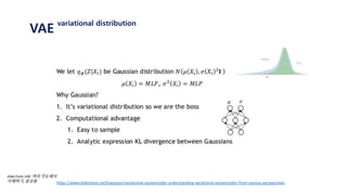
![𝐸𝑧~𝑝(𝑧)[log 𝑝 𝑥𝑖 𝑔 𝜃 𝑧 ]
= 𝑗=1
𝑀
𝑝 𝑥𝑖 𝑔 𝜃 𝑧𝑗 , 𝑧~𝑝(𝑧)
1. 표준정규분포 𝑝(𝑧) 에서 𝑧𝑗 를 셈플링한다.
2. 뉴럴넷을 통해 얻은 값인 𝑔 𝜃 𝑧𝑗 와
실제 𝑥𝑖 가 가까워지도록 gradient descent를 진행한다.
3. 위 과정을 i와 j에 대하여 계속 반복한다.
VAE
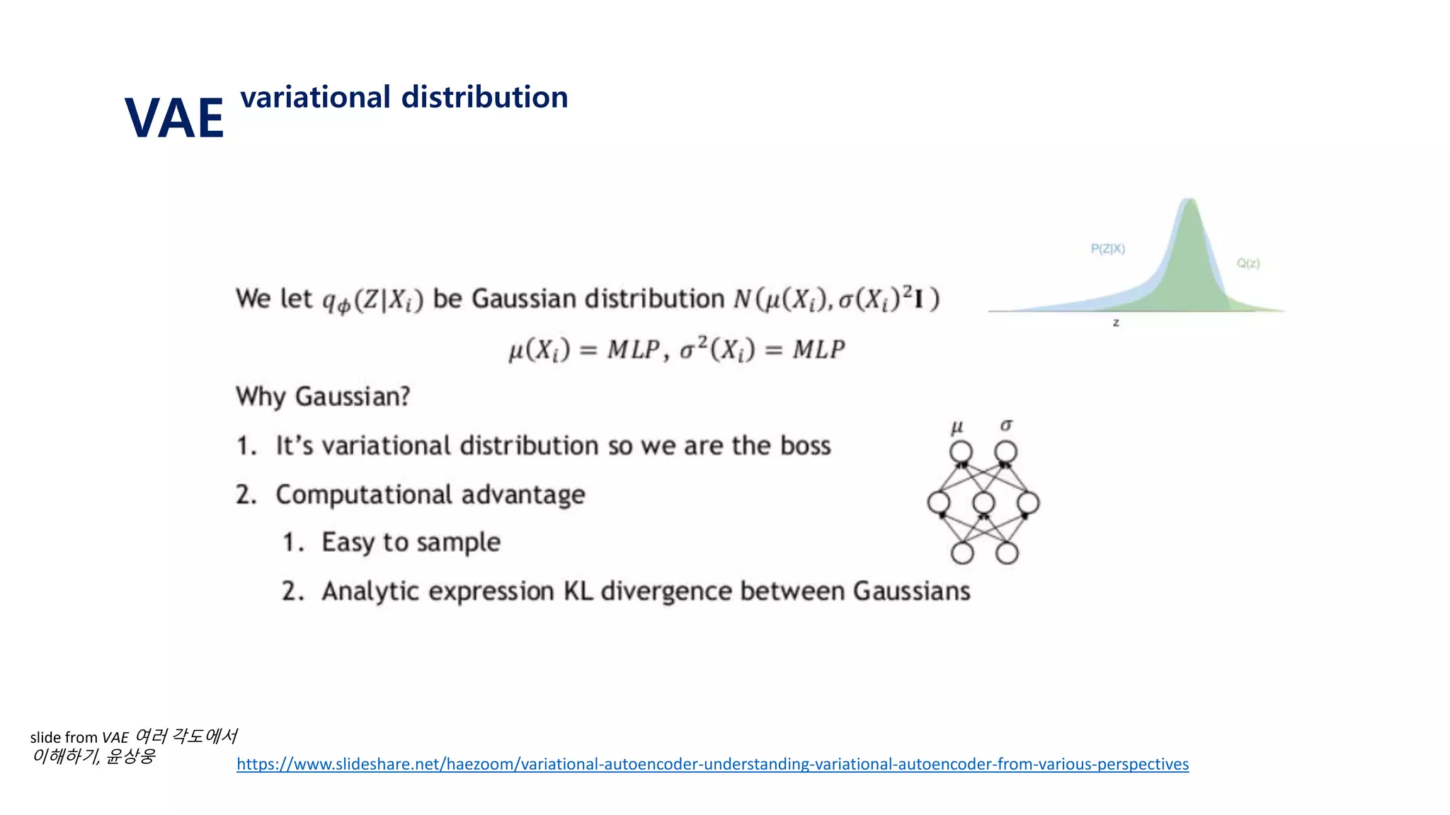
variational distribution](https://image.slidesharecdn.com/180208tutorialonvaelabseminar-180720033633/85/Variational-Autoencoder-Tutorial-38-320.jpg)
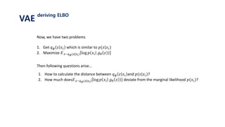
![Let’s use𝐸𝑧~𝑝(𝑧|𝑥 𝑖) log 𝑝 𝑥𝑖 𝑔 𝜃 𝑧 instead of 𝐸𝑧~𝑝(𝑧)
We can now get “differentiating” samples!
However, 𝑝 𝑧 𝑥𝑖 is intractable(cannot calculate)
Therefore, we go variational.
We approximate the posterior 𝑝 𝑧 𝑥𝑖
𝐸𝑧~𝑝(𝑧)[log 𝑝 𝑥𝑖 𝑔 𝜃 𝑧 ]
= 𝑗=1
𝑀
𝑝 𝑥𝑖 𝑔 𝜃 𝑧𝑗 , 𝑧~𝑝(𝑧)
즉, 𝑥𝑖가 주어지면
𝑝 𝑧 𝑥𝑖 에서 𝑧를 𝑠𝑎𝑚𝑝𝑙𝑖𝑛𝑔한 뒤
𝑔 𝜃 𝑧 를 구한 후
𝑥𝑖와 𝑔 𝜃 𝑧 를 비교한다.1. 표준정규분포 𝑝(𝑧) 에서 𝑧𝑗 를 셈플링한다.
2. 뉴럴넷을 통해 얻은 값인 𝑔 𝜃 𝑧𝑗 와
실제 𝑥𝑖 가 가까워지도록 gradient descent를 진행한다.
3. 위 과정을 i와 j에 대하여 계속 반복한다.
VAE
variational distribution](https://image.slidesharecdn.com/180208tutorialonvaelabseminar-180720033633/85/Variational-Autoencoder-Tutorial-39-320.jpg)
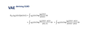
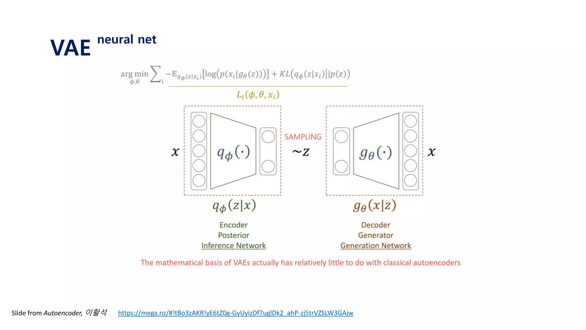
![Since we will never know the posterior 𝑝 𝑧 𝑥𝑖
We approximate it with variational distribution 𝑞 𝜙 𝑧 𝑥𝑖
𝐿 𝑥𝑖 ≅ 𝐸𝑧~𝑝(𝑧)[log 𝑝 𝑥𝑖 𝑔 𝜃 𝑧 ]
𝐿 𝑥𝑖 ≅ 𝐸𝑧~𝑝(𝑧|𝑥 𝑖)[log 𝑝 𝑥𝑖 𝑔 𝜃 𝑧 ]
𝐿 𝑥𝑖 ≅ 𝐸𝑧~𝑞 𝜙(𝑧|𝑥 𝑖)[log 𝑝 𝑥𝑖 𝑔 𝜃 𝑧 ]
With sufficiently good 𝑞 𝜙(𝑧|𝑥𝑖), we will get better gradients
VAE
variational distribution](https://image.slidesharecdn.com/180208tutorialonvaelabseminar-180720033633/85/Variational-Autoencoder-Tutorial-40-320.jpg)


![𝐿 𝑊, 𝑏, 𝑊, 𝑏 =
𝑛=1
𝑁
𝑥 𝑛 − 𝑥 𝑥 𝑛
2
If the shape of W is [n,m],
than the shape of 𝑊 is [m,n]
𝑦𝑛
Generally, 𝑊 is not 𝑊 𝑇,
but weight sharing is also possible!
(to reduce the number of parameters)
𝑦1
Autoencoder](https://image.slidesharecdn.com/180208tutorialonvaelabseminar-180720033633/75/Variational-Autoencoder-Tutorial-4-2048.jpg)


![input
𝑥
output
𝑓𝜃(𝑥)
data parameter
𝑦𝑓𝜃1 𝑥
𝑝(𝑦| 𝑓𝜃1 𝑥 )𝑚𝑎𝑥𝑖𝑚𝑖𝑧𝑒 𝒑 𝜽 𝒚 𝒙 𝑜𝑟 𝒑 𝒚 𝒇 𝜽 𝒙
𝑚𝑖𝑛𝑖𝑚𝑖𝑧𝑒 − 𝐥𝐨𝐠[𝒑 𝒚 𝒇 𝜽 𝒙 ]
VAE
Explicit density model
assume that 𝑝 𝜃 𝑦 𝑥 follows normal distribution, N(𝑓𝜃 𝑥 , 1)
find 𝑓𝜃 𝑥 that maximize 𝑝 𝜃 𝑦 𝑥 using neural net
Actually, we do this using neural Net!
The output of neural net is parameter of distribution
N(𝑓𝜃 𝑥 , 1) 인 정규분포에서 데이터 y가 나올 확률밀도 값을 얻을 수 있음, 𝒑 𝒚 𝒇 𝜽 𝒙
이를 최대화 하는 방향으로 업데이트!](https://image.slidesharecdn.com/180208tutorialonvaelabseminar-180720033633/75/Variational-Autoencoder-Tutorial-14-2048.jpg)
![input
𝑥
output
𝑓𝜃(𝑥)
data parameter
𝑦𝑓𝜃1 𝑥
𝑝(𝑦| 𝑓𝜃1 𝑥 ) <
𝑓𝜃2 𝑥
𝑝(𝑦| 𝑓𝜃2 𝑥 )𝑚𝑎𝑥𝑖𝑚𝑖𝑧𝑒 𝒑 𝜽 𝒚 𝒙 𝑜𝑟 𝒑 𝒚 𝒇 𝜽 𝒙
𝑚𝑖𝑛𝑖𝑚𝑖𝑧𝑒 − 𝐥𝐨𝐠[𝒑 𝒚 𝒇 𝜽 𝒙 ]
VAE
Explicit density model
assume that 𝑝 𝜃 𝑦 𝑥 follows normal distribution, N(𝑓𝜃 𝑥 , 1)
find 𝑓𝜃 𝑥 that maximize 𝑝 𝜃 𝑦 𝑥 using neural net
Actually, we do this using neural Net!
The output of neural net is parameter of distribution](https://image.slidesharecdn.com/180208tutorialonvaelabseminar-180720033633/75/Variational-Autoencoder-Tutorial-15-2048.jpg)
![input
𝑥
output
𝑓𝜃(𝑥)
data parameter
𝑦𝑓𝜃1 𝑥 𝑓𝜃2 𝑥 = 𝑓𝜃3 𝑥
𝑚𝑎𝑥𝑖𝑚𝑖𝑧𝑒 𝒑 𝜽 𝒚 𝒙 𝑜𝑟 𝒑 𝒚 𝒇 𝜽 𝒙
𝑚𝑖𝑛𝑖𝑚𝑖𝑧𝑒 − 𝐥𝐨𝐠[𝒑 𝒚 𝒇 𝜽 𝒙 ]
VAE
Explicit density model
assume that 𝑝 𝜃 𝑦 𝑥 follows normal distribution, N(𝑓𝜃 𝑥 , 1)
find 𝑓𝜃 𝑥 that maximize 𝑝 𝜃 𝑦 𝑥 using neural net
Actually, we do this using neural Net!
The output of neural net is parameter of distribution](https://image.slidesharecdn.com/180208tutorialonvaelabseminar-180720033633/75/Variational-Autoencoder-Tutorial-16-2048.jpg)


![𝐿 𝑥𝑖 = log 𝑝( 𝑥𝑖)
Let’s use latent variable 𝑧 that follows standard normal distribution N(0, 𝑰)
Let’s assume that 𝒑 𝜽 𝒙 𝒛 𝑜𝑟 𝒑 𝒙 𝒈 𝜽 𝒛 is gaussian with N(𝒈 𝜽 𝒛 , 𝑰) ≈ log 𝑝 𝜃(𝑥𝑖|𝑧)𝑝(𝑧) 𝑑𝑧
= log 𝑝(𝑥𝑖| 𝑔 𝜃 𝑧 )𝑝(𝑧) 𝑑𝑧
= log 𝐸𝑧~𝑝(𝑧)[𝑝 𝑥𝑖 𝑔 𝜃 𝑧 ]
≥ 𝐸𝑧~𝑝(𝑧)[log 𝑝 𝑥𝑖 𝑔 𝜃 𝑧 ]
=
1
𝑀 𝑗=1
𝑀
log 𝑝 𝑥𝑖 𝑔 𝜃 𝑧𝑗 , 𝑧~𝑝(𝑧)
1. 표준정규분포 𝑝(𝑧) 에서 𝑧𝑗 를 셈플링한다.
2. 뉴럴넷을 통해 얻은 값인 𝑔 𝜃 𝑧𝑗 와 실제 𝑥𝑖 가 가까워지도록 gradient descent를 진행한다.
3. 위 과정을 i와 j에 대하여 계속 반복한다.
VAE
Naïve attempt](https://image.slidesharecdn.com/180208tutorialonvaelabseminar-180720033633/75/Variational-Autoencoder-Tutorial-29-2048.jpg)


![𝐸𝑧~𝑝(𝑧)[log 𝑝 𝑥𝑖 𝑔 𝜃 𝑧 ]
= 𝑗=1
𝑀
𝑝 𝑥𝑖 𝑔 𝜃 𝑧𝑗 , 𝑧~𝑝(𝑧)
1. 표준정규분포 𝑝(𝑧) 에서 𝑧𝑗 를 셈플링한다.
2. 뉴럴넷을 통해 얻은 값인 𝑔 𝜃 𝑧𝑗 와
실제 𝑥𝑖 가 가까워지도록 gradient descent를 진행한다.
3. 위 과정을 i와 j에 대하여 계속 반복한다.
VAE
variational distribution](https://image.slidesharecdn.com/180208tutorialonvaelabseminar-180720033633/75/Variational-Autoencoder-Tutorial-38-2048.jpg)
![Let’s use𝐸𝑧~𝑝(𝑧|𝑥 𝑖) log 𝑝 𝑥𝑖 𝑔 𝜃 𝑧 instead of 𝐸𝑧~𝑝(𝑧)
We can now get “differentiating” samples!
However, 𝑝 𝑧 𝑥𝑖 is intractable(cannot calculate)
Therefore, we go variational.
We approximate the posterior 𝑝 𝑧 𝑥𝑖
𝐸𝑧~𝑝(𝑧)[log 𝑝 𝑥𝑖 𝑔 𝜃 𝑧 ]
= 𝑗=1
𝑀
𝑝 𝑥𝑖 𝑔 𝜃 𝑧𝑗 , 𝑧~𝑝(𝑧)
즉, 𝑥𝑖가 주어지면
𝑝 𝑧 𝑥𝑖 에서 𝑧를 𝑠𝑎𝑚𝑝𝑙𝑖𝑛𝑔한 뒤
𝑔 𝜃 𝑧 를 구한 후
𝑥𝑖와 𝑔 𝜃 𝑧 를 비교한다.1. 표준정규분포 𝑝(𝑧) 에서 𝑧𝑗 를 셈플링한다.
2. 뉴럴넷을 통해 얻은 값인 𝑔 𝜃 𝑧𝑗 와
실제 𝑥𝑖 가 가까워지도록 gradient descent를 진행한다.
3. 위 과정을 i와 j에 대하여 계속 반복한다.
VAE
variational distribution](https://image.slidesharecdn.com/180208tutorialonvaelabseminar-180720033633/75/Variational-Autoencoder-Tutorial-39-2048.jpg)
![Since we will never know the posterior 𝑝 𝑧 𝑥𝑖
We approximate it with variational distribution 𝑞 𝜙 𝑧 𝑥𝑖
𝐿 𝑥𝑖 ≅ 𝐸𝑧~𝑝(𝑧)[log 𝑝 𝑥𝑖 𝑔 𝜃 𝑧 ]
𝐿 𝑥𝑖 ≅ 𝐸𝑧~𝑝(𝑧|𝑥 𝑖)[log 𝑝 𝑥𝑖 𝑔 𝜃 𝑧 ]
𝐿 𝑥𝑖 ≅ 𝐸𝑧~𝑞 𝜙(𝑧|𝑥 𝑖)[log 𝑝 𝑥𝑖 𝑔 𝜃 𝑧 ]
With sufficiently good 𝑞 𝜙(𝑧|𝑥𝑖), we will get better gradients
VAE
variational distribution](https://image.slidesharecdn.com/180208tutorialonvaelabseminar-180720033633/75/Variational-Autoencoder-Tutorial-40-2048.jpg)


![[DL輪読会]Deep Learning 第5章 機械学習の基礎](https://cdn.slidesharecdn.com/ss_thumbnails/deeplearning5-180601021956-thumbnail.jpg?width=600ounds&width=560&fit=bounds)


![[AIoTLab]attention mechanism.pptx](https://cdn.slidesharecdn.com/ss_thumbnails/aiotlabattentionmechanism-230406114603-e5ba0365-thumbnail.jpg?width=600ounds&width=560&fit=bounds)


