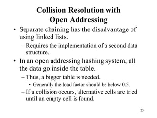
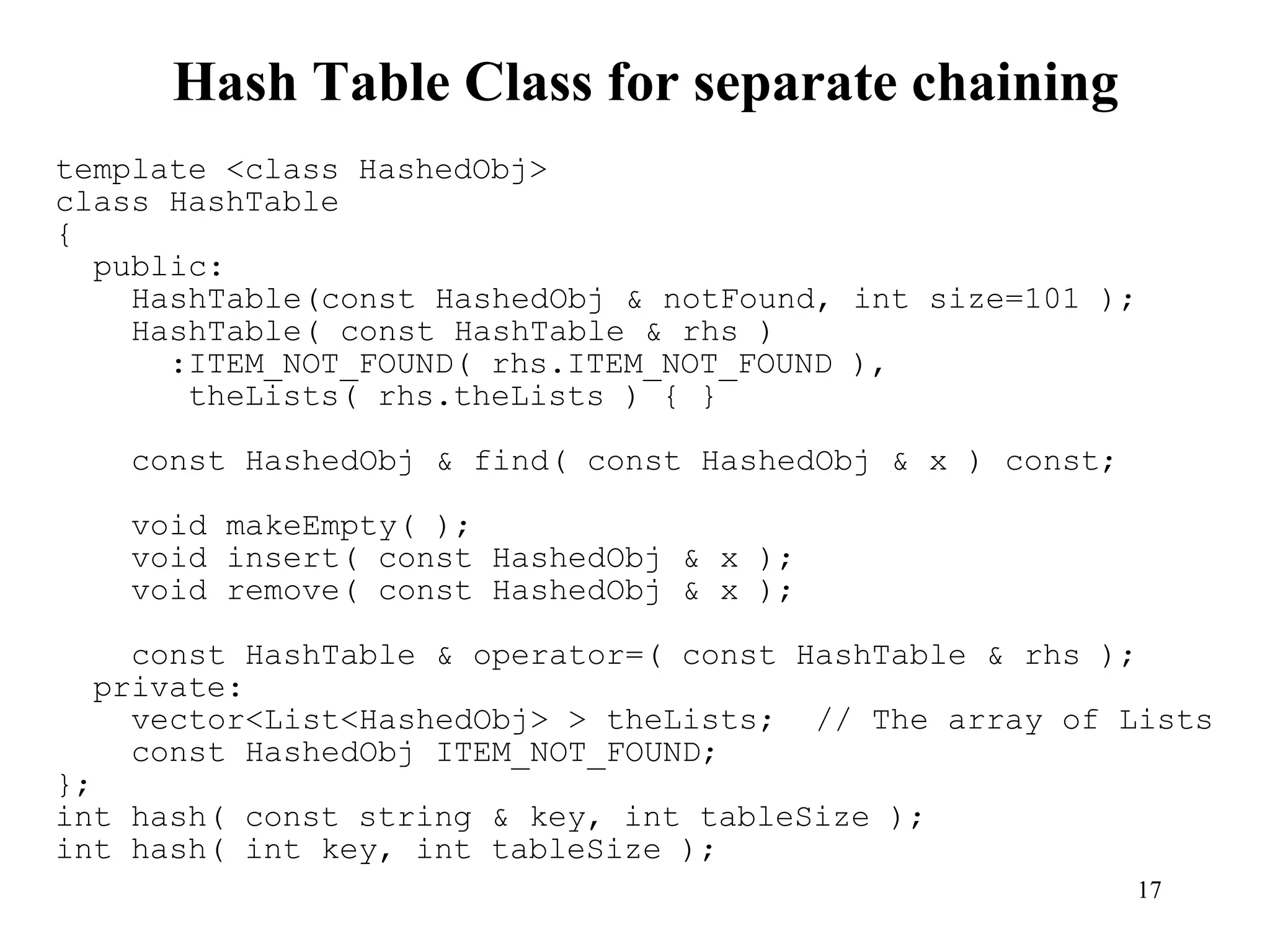
Hash tables provide constant time insertion, deletion and search by using a hash function to map keys to indexes in an array. Collisions occur when different keys hash to the same index. Separate chaining resolves collisions by storing keys in linked lists at each index. Open addressing resolves collisions by probing to the next index using functions like linear probing. The load factor and choice of hash function impact performance.


![9
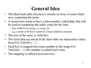
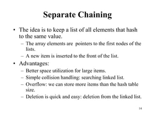
Hash Function 1
• Add up the ASCII values of all characters of the key.
int hash(const string &key, int tableSize)
{
int hasVal = 0;
for (int i = 0; i < key.length(); i++)
hashVal += key[i];
return hashVal % tableSize;
}
• Simple to implement and fast.
• However, if the table size is large, the function does not
distribute the keys well.
• e.g. Table size =10000, key length <= 8, the hash function can
assume values only between 0 and 1016](https://image.slidesharecdn.com/11hashtable-1-240305184500-c9454bd1/85/11_hashtable-1-ppt-Data-structure-algorithm-9-320.jpg)
![10
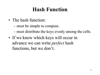
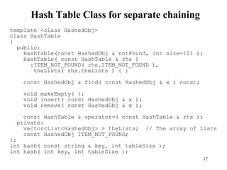
Hash Function 2
• Examine only the first 3 characters of the key.
int hash (const string &key, int tableSize)
{
return (key[0]+27 * key[1] + 729*key[2]) % tableSize;
}
• In theory, 26 * 26 * 26 = 17576 different words can be
generated. However, English is not random, only 2851
different combinations are possible.
• Thus, this function although easily computable, is also not
appropriate if the hash table is reasonably large.](https://image.slidesharecdn.com/11hashtable-1-240305184500-c9454bd1/85/11_hashtable-1-ppt-Data-structure-algorithm-10-320.jpg)
![11
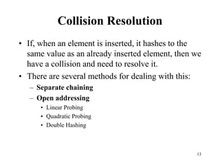
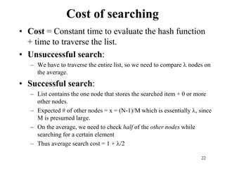
Hash Function 3
int hash (const string &key, int tableSize)
{
int hashVal = 0;
for (int i = 0; i < key.length(); i++)
hashVal = 37 * hashVal + key[i];
hashVal %=tableSize;
if (hashVal < 0) /* in case overflows occurs */
hashVal += tableSize;
return hashVal;
};
1
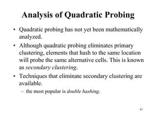
0
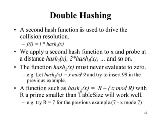
37
]
1
[
)
(
KeySize
i
i
i
KeySize
Key
key
hash](https://image.slidesharecdn.com/11hashtable-1-240305184500-c9454bd1/85/11_hashtable-1-ppt-Data-structure-algorithm-11-320.jpg)
![12
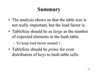
Hash function for strings:
a l i
key
KeySize = 3;
98 108 105
hash(“ali”) = (105 * 1 + 108*37 + 98*372) % 10,007 = 8172
0 1 2 i
key[i]
hash
function
ali
……
……
0
1
2
8172
10,006 (TableSize)
“ali”](https://image.slidesharecdn.com/11hashtable-1-240305184500-c9454bd1/85/11_hashtable-1-ppt-Data-structure-algorithm-12-320.jpg)


![18
Insert routine
/**
* Insert item x into the hash table. If the item is
* already present, then do nothing.
*/
template <class HashedObj>
void HashTable<HashedObj>::insert(const HashedObj & x )
{
List<HashedObj> & whichList = theLists[ hash( x,
theLists.size( ) ) ];
HashedObj* p = whichList.find( x );
if( p == NULL )
whichList.insert( x, whichList.zeroth( ) );
}](https://image.slidesharecdn.com/11hashtable-1-240305184500-c9454bd1/85/11_hashtable-1-ppt-Data-structure-algorithm-18-320.jpg)
![19
Remove routine
/**
* Remove item x from the hash table.
*/
template <class HashedObj>
void HashTable<HashedObj>::remove( const HashedObj & x )
{
theLists[hash(x, theLists.size())].remove( x );
}](https://image.slidesharecdn.com/11hashtable-1-240305184500-c9454bd1/85/11_hashtable-1-ppt-Data-structure-algorithm-19-320.jpg)
![20
Find routine
/**
* Find item x in the hash table.
* Return the matching item or ITEM_NOT_FOUND if not found
*/
template <class HashedObj>
const HashedObj & HashTable<HashedObj>::find( const
HashedObj & x ) const
{
HashedObj * itr;
itr = theLists[ hash( x, theLists.size( ) ) ].find( x );
if(itr==NULL)
return ITEM_NOT_FOUND;
else
return *itr;
}](https://image.slidesharecdn.com/11hashtable-1-240305184500-c9454bd1/85/11_hashtable-1-ppt-Data-structure-algorithm-20-320.jpg)


![47
Largest Subset w/ Consecutive Numbers
Input: 1,3,8,14,4,10,2,11 Output: 1,2,3,4
Complexity analyses of 3 solutions
1) Naïve: for each element e, set a=e search for a+1 then a++: O(n2)
2) Sorting: Get 1,2,3,4,8,10,11,14. Start in 1, track until 4 (size=4);
restart in 8, track until 10; restart in 10, track until 14 (size=2); restart
in 14. Note that sorted array traversed once: O(nlogn + n) = O(nlogn)
3) Hashing: for each cluster of size k, we do
k successful find() by the starter (+1s)
Other k-1 nonstarter members find() left element (-1)
Total cost is hence k+k-1 = 2k-1
[ C1 ][C2][ C3 ][ C4 ][ C5 ] ∑ (2ki - 1) = 2∑ ki - #clusters
i i
= 2n - #clusters = O(n) //worst: 1 huge cluster 2n-1; best: n clusters (each size 1) 2n-n](https://image.slidesharecdn.com/11hashtable-1-240305184500-c9454bd1/85/11_hashtable-1-ppt-Data-structure-algorithm-47-320.jpg)


![9
Hash Function 1
• Add up the ASCII values of all characters of the key.
int hash(const string &key, int tableSize)
{
int hasVal = 0;
for (int i = 0; i < key.length(); i++)
hashVal += key[i];
return hashVal % tableSize;
}
• Simple to implement and fast.
• However, if the table size is large, the function does not
distribute the keys well.
• e.g. Table size =10000, key length <= 8, the hash function can
assume values only between 0 and 1016](https://image.slidesharecdn.com/11hashtable-1-240305184500-c9454bd1/75/11_hashtable-1-ppt-Data-structure-algorithm-9-2048.jpg)
![10
Hash Function 2
• Examine only the first 3 characters of the key.
int hash (const string &key, int tableSize)
{
return (key[0]+27 * key[1] + 729*key[2]) % tableSize;
}
• In theory, 26 * 26 * 26 = 17576 different words can be
generated. However, English is not random, only 2851
different combinations are possible.
• Thus, this function although easily computable, is also not
appropriate if the hash table is reasonably large.](https://image.slidesharecdn.com/11hashtable-1-240305184500-c9454bd1/75/11_hashtable-1-ppt-Data-structure-algorithm-10-2048.jpg)
![11
Hash Function 3
int hash (const string &key, int tableSize)
{
int hashVal = 0;
for (int i = 0; i < key.length(); i++)
hashVal = 37 * hashVal + key[i];
hashVal %=tableSize;
if (hashVal < 0) /* in case overflows occurs */
hashVal += tableSize;
return hashVal;
};
1
0
37
]
1
[
)
(
KeySize
i
i
i
KeySize
Key
key
hash](https://image.slidesharecdn.com/11hashtable-1-240305184500-c9454bd1/75/11_hashtable-1-ppt-Data-structure-algorithm-11-2048.jpg)
![12
Hash function for strings:
a l i
key
KeySize = 3;
98 108 105
hash(“ali”) = (105 * 1 + 108*37 + 98*372) % 10,007 = 8172
0 1 2 i
key[i]
hash
function
ali
……
……
0
1
2
8172
10,006 (TableSize)
“ali”](https://image.slidesharecdn.com/11hashtable-1-240305184500-c9454bd1/75/11_hashtable-1-ppt-Data-structure-algorithm-12-2048.jpg)

![18
Insert routine
/**
* Insert item x into the hash table. If the item is
* already present, then do nothing.
*/
template <class HashedObj>
void HashTable<HashedObj>::insert(const HashedObj & x )
{
List<HashedObj> & whichList = theLists[ hash( x,
theLists.size( ) ) ];
HashedObj* p = whichList.find( x );
if( p == NULL )
whichList.insert( x, whichList.zeroth( ) );
}](https://image.slidesharecdn.com/11hashtable-1-240305184500-c9454bd1/75/11_hashtable-1-ppt-Data-structure-algorithm-18-2048.jpg)
![19
Remove routine
/**
* Remove item x from the hash table.
*/
template <class HashedObj>
void HashTable<HashedObj>::remove( const HashedObj & x )
{
theLists[hash(x, theLists.size())].remove( x );
}](https://image.slidesharecdn.com/11hashtable-1-240305184500-c9454bd1/75/11_hashtable-1-ppt-Data-structure-algorithm-19-2048.jpg)
![20
Find routine
/**
* Find item x in the hash table.
* Return the matching item or ITEM_NOT_FOUND if not found
*/
template <class HashedObj>
const HashedObj & HashTable<HashedObj>::find( const
HashedObj & x ) const
{
HashedObj * itr;
itr = theLists[ hash( x, theLists.size( ) ) ].find( x );
if(itr==NULL)
return ITEM_NOT_FOUND;
else
return *itr;
}](https://image.slidesharecdn.com/11hashtable-1-240305184500-c9454bd1/75/11_hashtable-1-ppt-Data-structure-algorithm-20-2048.jpg)


![47
Largest Subset w/ Consecutive Numbers
Input: 1,3,8,14,4,10,2,11 Output: 1,2,3,4
Complexity analyses of 3 solutions
1) Naïve: for each element e, set a=e search for a+1 then a++: O(n2)
2) Sorting: Get 1,2,3,4,8,10,11,14. Start in 1, track until 4 (size=4);
restart in 8, track until 10; restart in 10, track until 14 (size=2); restart
in 14. Note that sorted array traversed once: O(nlogn + n) = O(nlogn)
3) Hashing: for each cluster of size k, we do
k successful find() by the starter (+1s)
Other k-1 nonstarter members find() left element (-1)
Total cost is hence k+k-1 = 2k-1
[ C1 ][C2][ C3 ][ C4 ][ C5 ] ∑ (2ki - 1) = 2∑ ki - #clusters
i i
= 2n - #clusters = O(n) //worst: 1 huge cluster 2n-1; best: n clusters (each size 1) 2n-n](https://image.slidesharecdn.com/11hashtable-1-240305184500-c9454bd1/75/11_hashtable-1-ppt-Data-structure-algorithm-47-2048.jpg)


