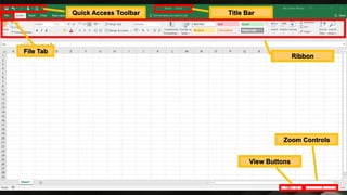
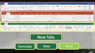
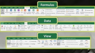
This document describes Empowerment Technologies, a tool for financial analysis, modeling, and collaboration. It features calculation and graphing tools, pivot tables, and a macro programming language. It can compute costs, create tables and findings, and generate reports for business or research projects. It is also a collaboration tool for financial analysis or modeling.
It features calculation,graphing tools, pivot tables, and a
macro programming language.
It can compute costs incurred in the creation of projects,
or create tables for findings in the researchers, and then create
reports for business or research that you are doing.
It is also a collaboration tool for financial analysis or
modelling.
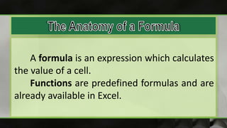
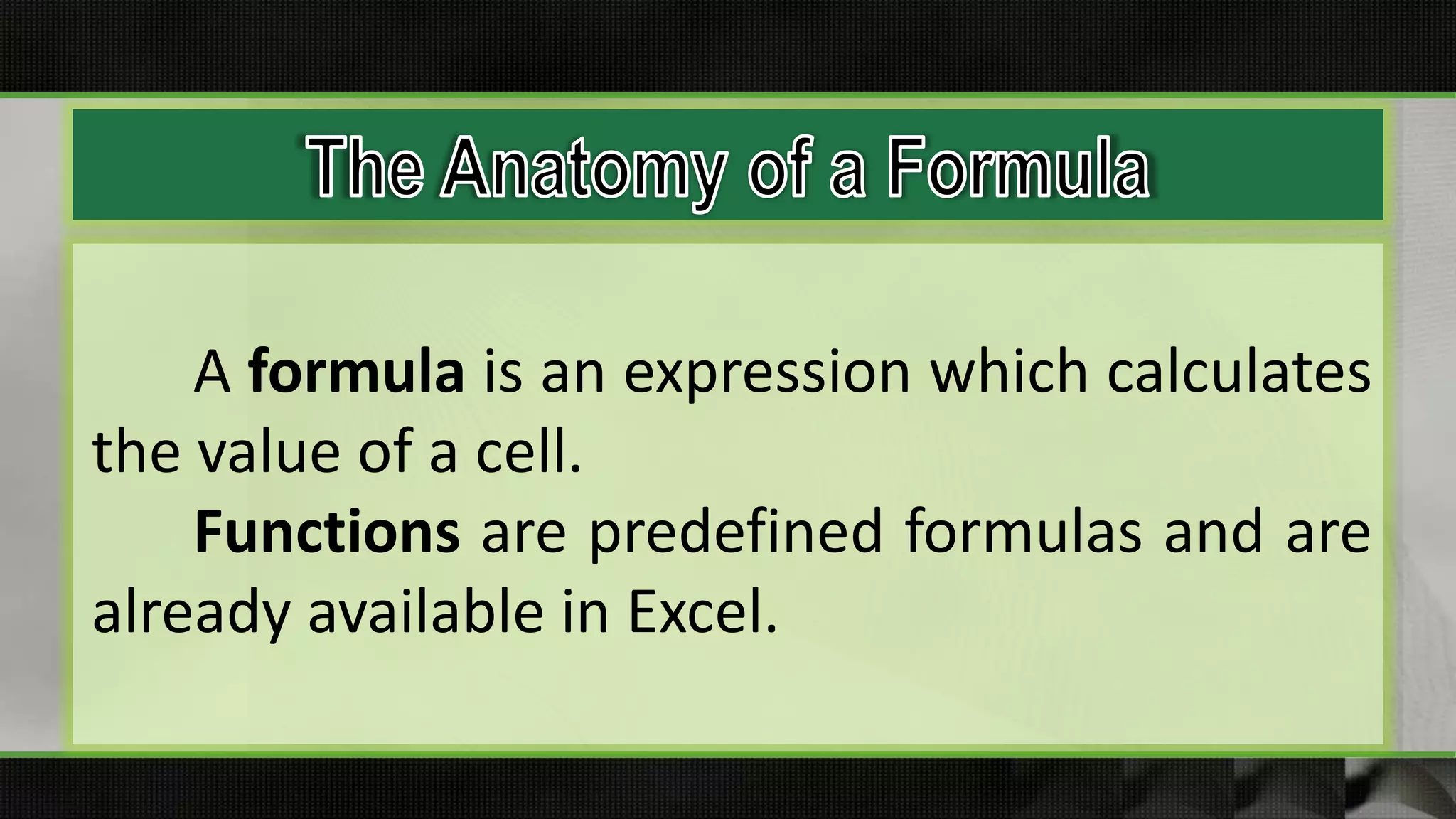
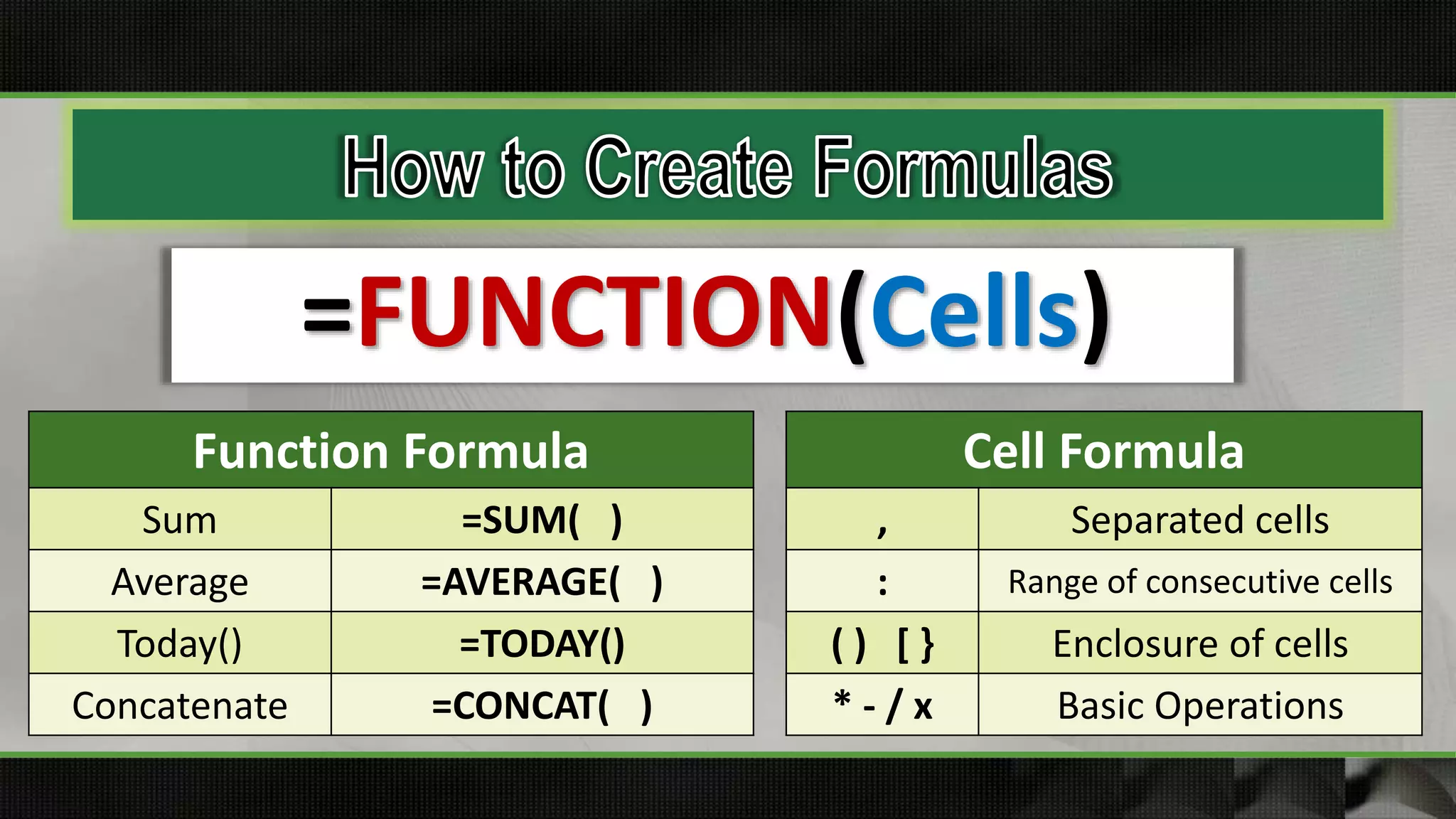
A formula isan expression which calculates
the value of a cell.
Functions are predefined formulas and are
already available in Excel.
9.
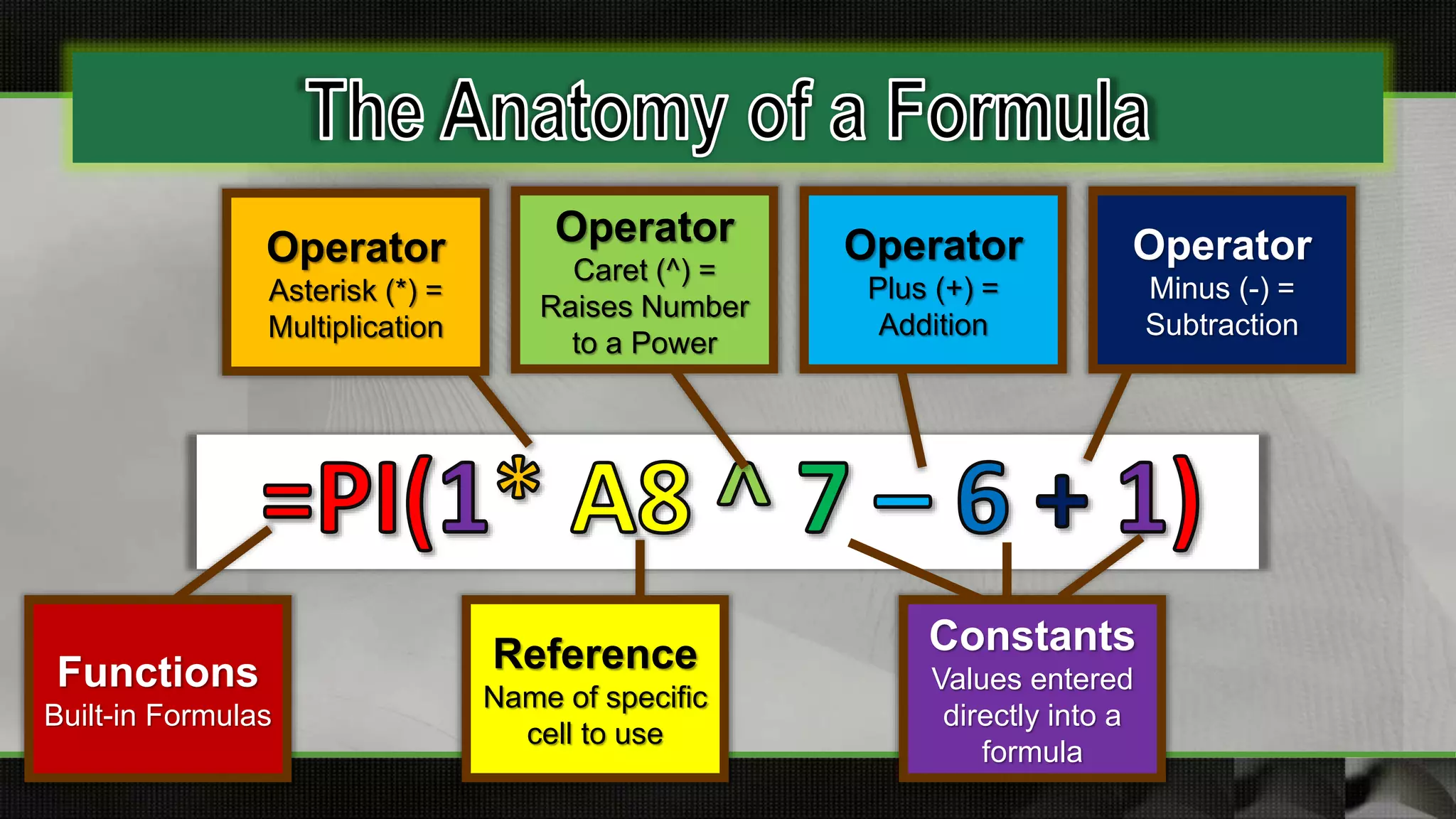
Functions
Built-in Formulas
Operator
Asterisk (*)=
Multiplication
Operator
Caret (^) =
Raises Number
to a Power
Operator
Plus (+) =
Addition
Operator
Minus (-) =
Subtraction
Reference
Name of specific
cell to use
Constants
Values entered
directly into a
formula
10.
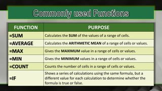
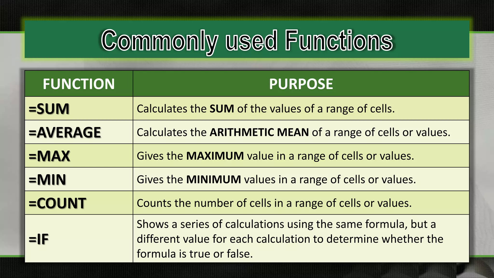
FUNCTION PURPOSE
=SUM Calculatesthe SUM of the values of a range of cells.
=AVERAGE Calculates the ARITHMETIC MEAN of a range of cells or values.
=MAX Gives the MAXIMUM value in a range of cells or values.
=MIN Gives the MINIMUM values in a range of cells or values.
=COUNT Counts the number of cells in a range of cells or values.
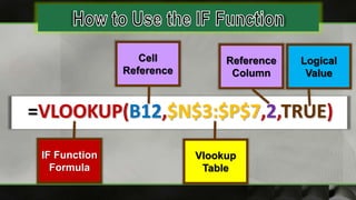
=IF
Shows a series of calculations using the same formula, but a
different value for each calculation to determine whether the
formula is true or false.
11.
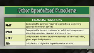
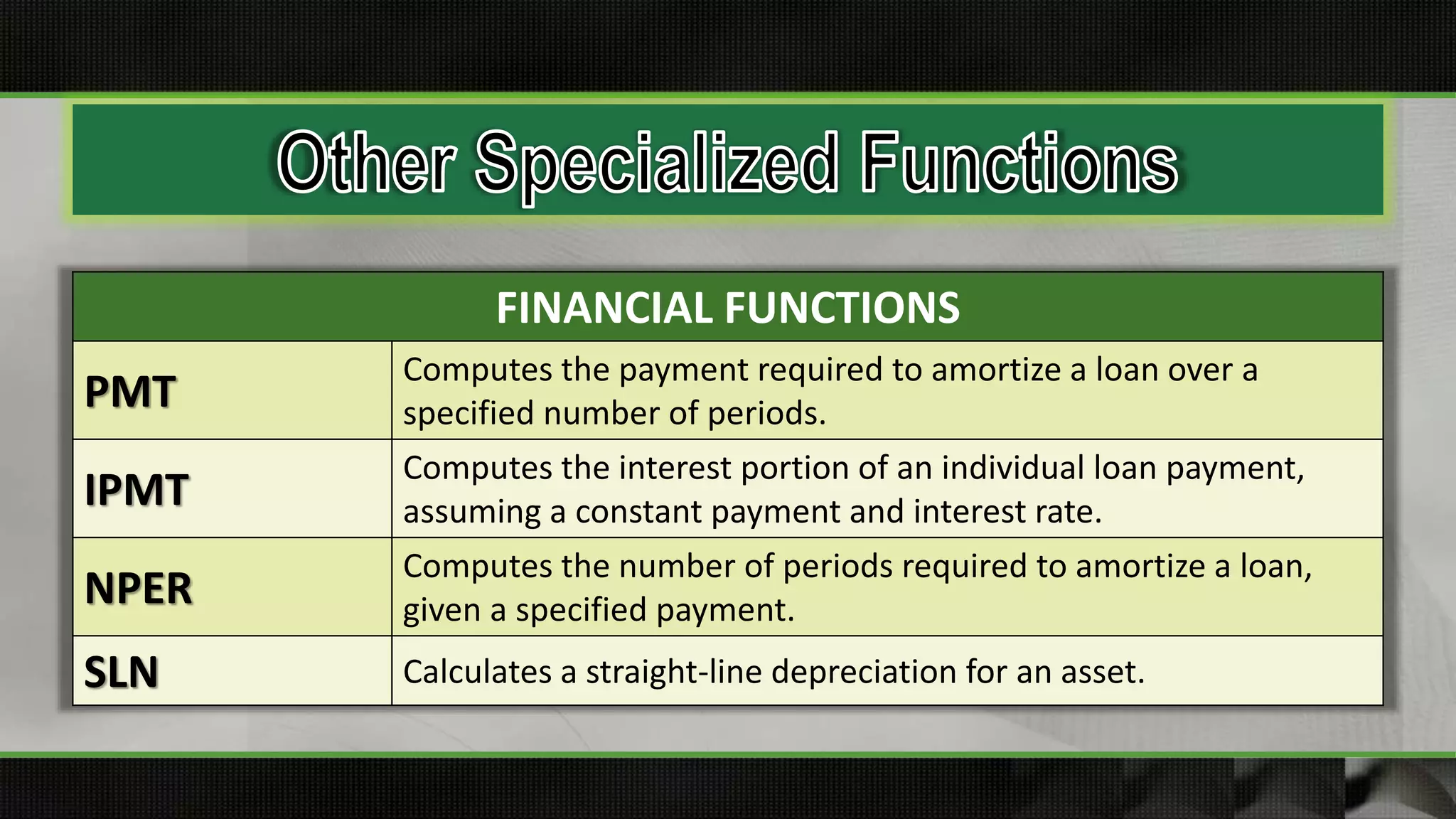
FINANCIAL FUNCTIONS
PMT
Computes thepayment required to amortize a loan over a
specified number of periods.
IPMT
Computes the interest portion of an individual loan payment,
assuming a constant payment and interest rate.
NPER
Computes the number of periods required to amortize a loan,
given a specified payment.
SLN Calculates a straight-line depreciation for an asset.
12.
LOGICAL FUNCTIONS
IF Appliesa logical test that results in a True or False.
Nested IF Creates a hierarchy of tests.
AND
Returns FALSE if any of its arguments are false, and returns TRUE
only if all of its arguments are true.
13.
TEXT FUNCTIONS
CLEAN Removesall nonprintable characters.
CONCATENATE Combines text from multiple fields into one cell.
EXACT Compares two text strings to see if they are the same.
LEFT Returns the first num_characters in a text string.
UPPER Converts text into all-uppercase characters (SHIFT + F3).
14.
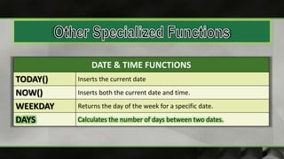
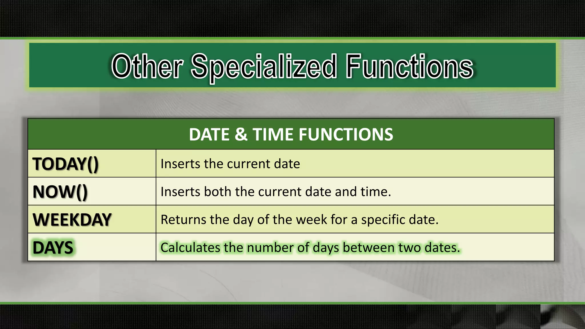
DATE & TIMEFUNCTIONS
TODAY() Inserts the current date
NOW() Inserts both the current date and time.
WEEKDAY Returns the day of the week for a specific date.
DAYS Calculates the number of days between two dates.
15.
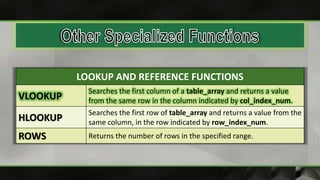
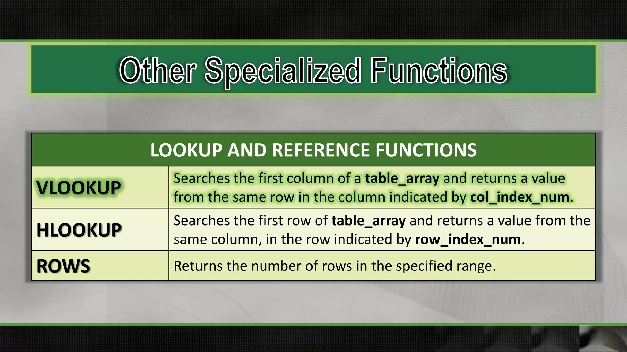
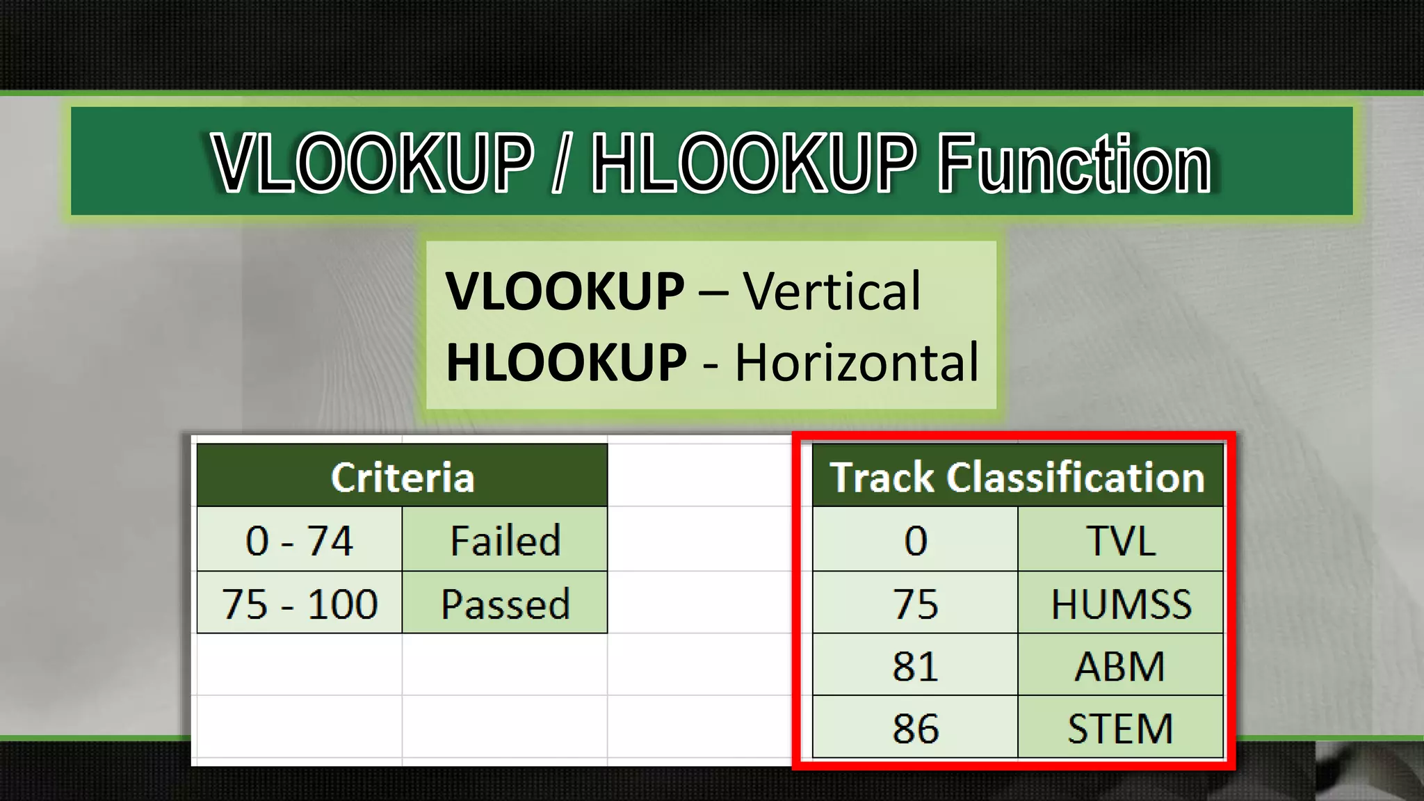
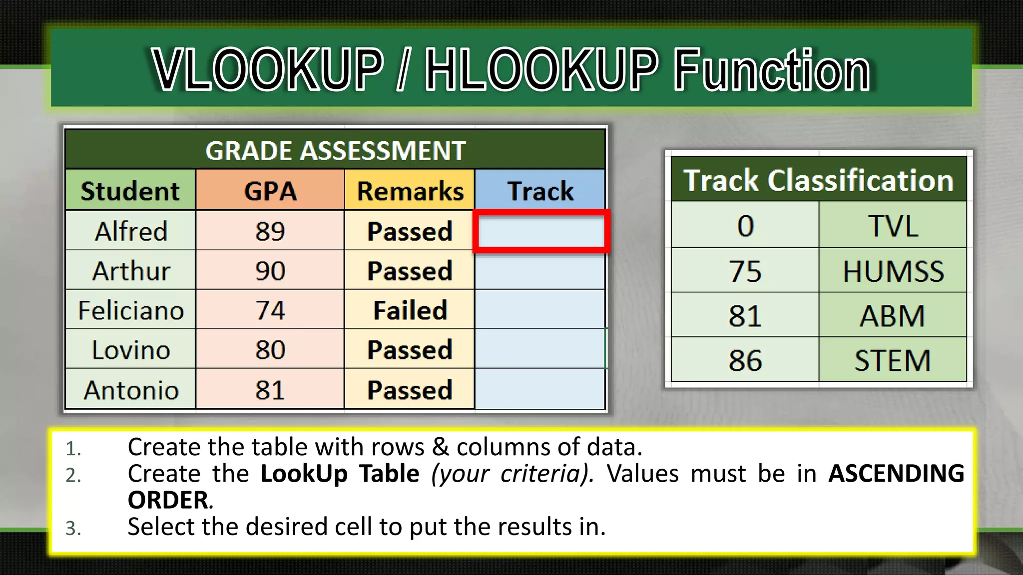
LOOKUP AND REFERENCEFUNCTIONS
VLOOKUP
Searches the first column of a table_array and returns a value
from the same row in the column indicated by col_index_num.
HLOOKUP
Searches the first row of table_array and returns a value from the
same column, in the row indicated by row_index_num.
ROWS Returns the number of rows in the specified range.
16.
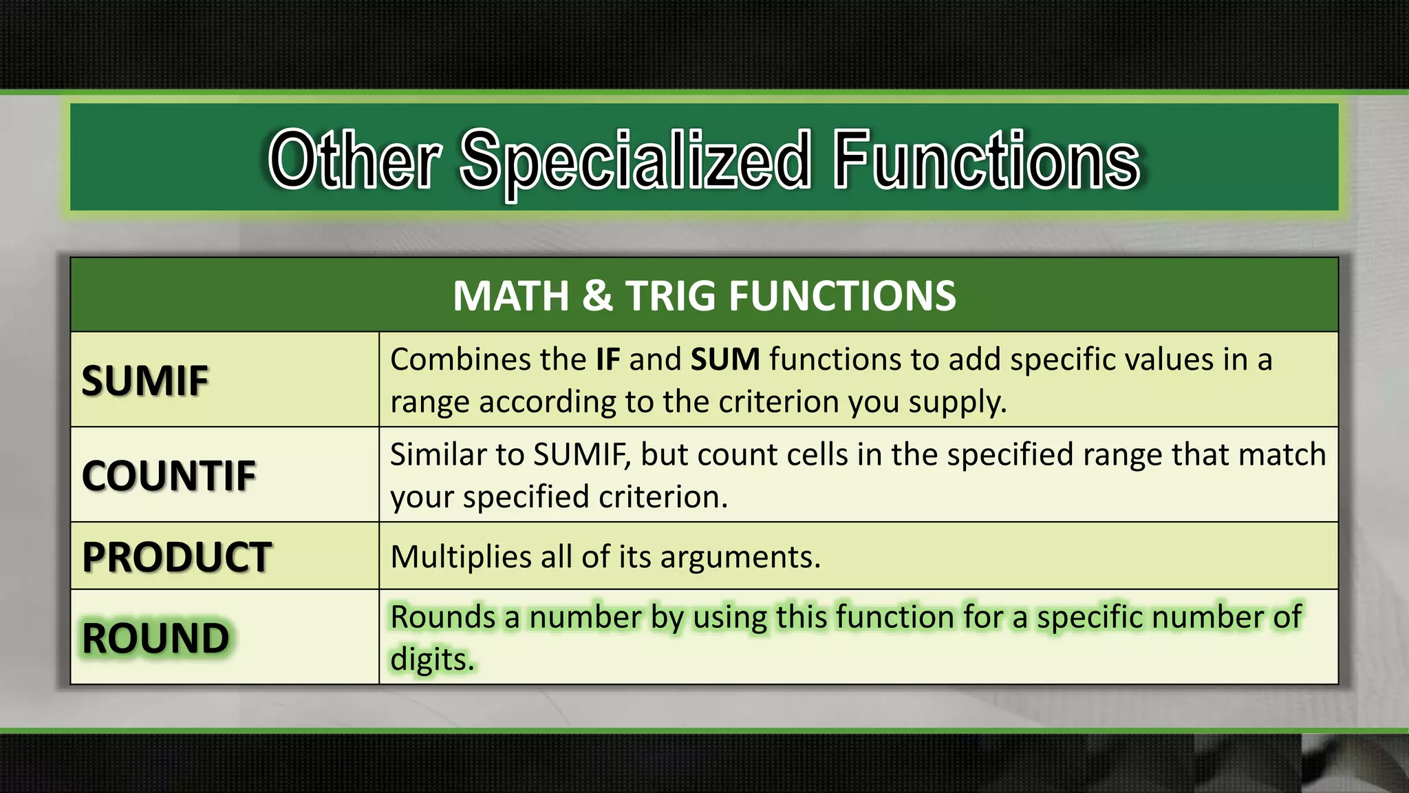
MATH & TRIGFUNCTIONS
SUMIF
Combines the IF and SUM functions to add specific values in a
range according to the criterion you supply.
COUNTIF
Similar to SUMIF, but count cells in the specified range that match
your specified criterion.
PRODUCT Multiplies all of its arguments.
ROUND
Rounds a number by using this function for a specific number of
digits.
17.
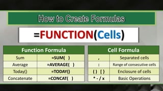
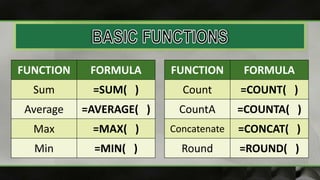
Function Formula
Sum =SUM()
Average =AVERAGE( )
Today() =TODAY()
Concatenate =CONCAT( )
=FUNCTION(Cells)
Cell Formula
, Separated cells
: Range of consecutive cells
( ) [ } Enclosure of cells
* - / x Basic Operations
18.
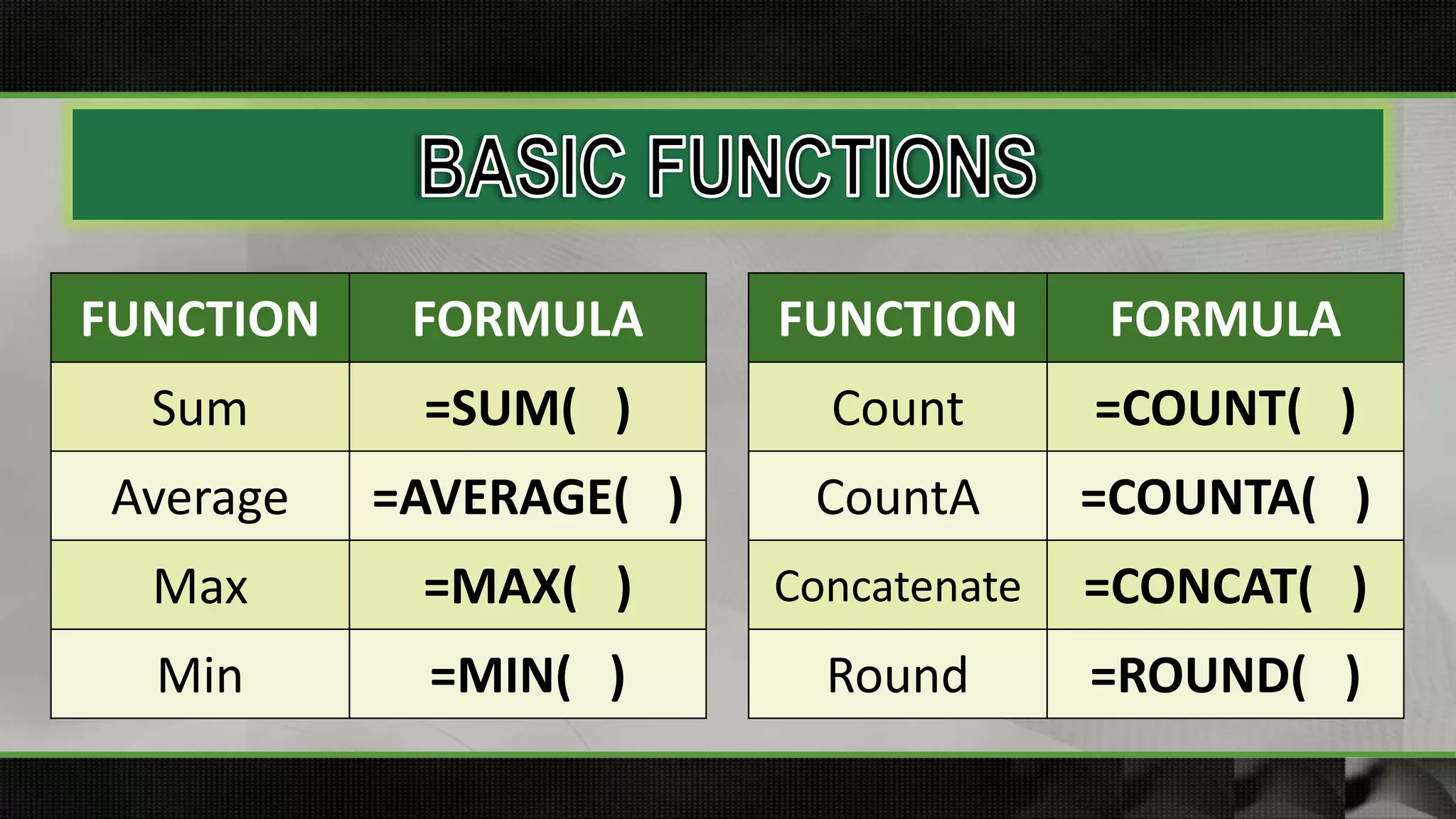
FUNCTION FORMULA
Sum =SUM()
Average =AVERAGE( )
Max =MAX( )
Min =MIN( )
FUNCTION FORMULA
Count =COUNT( )
CountA =COUNTA( )
Concatenate =CONCAT( )
Round =ROUND( )
19.
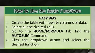
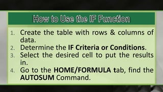
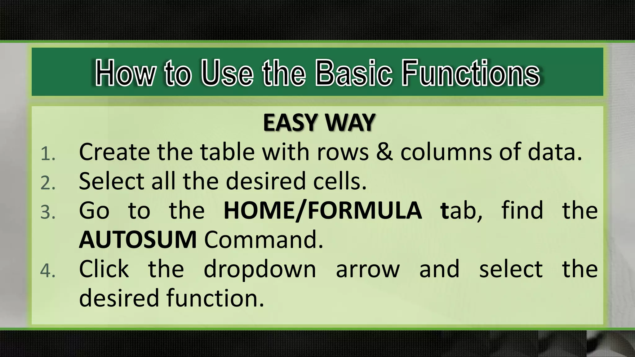
EASY WAY
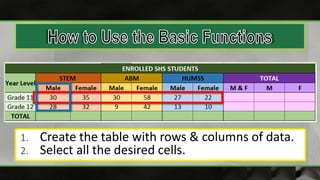
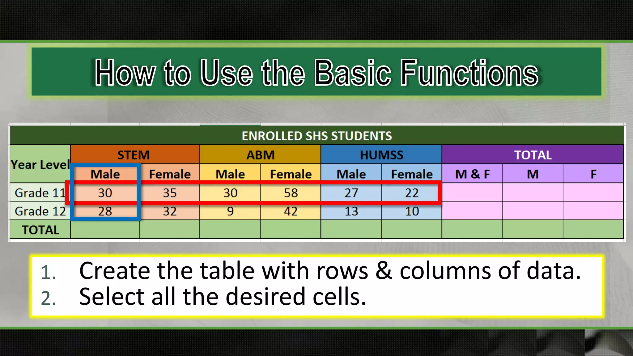
1. Createthe table with rows & columns of data.
2. Select all the desired cells.
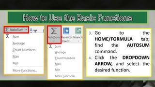
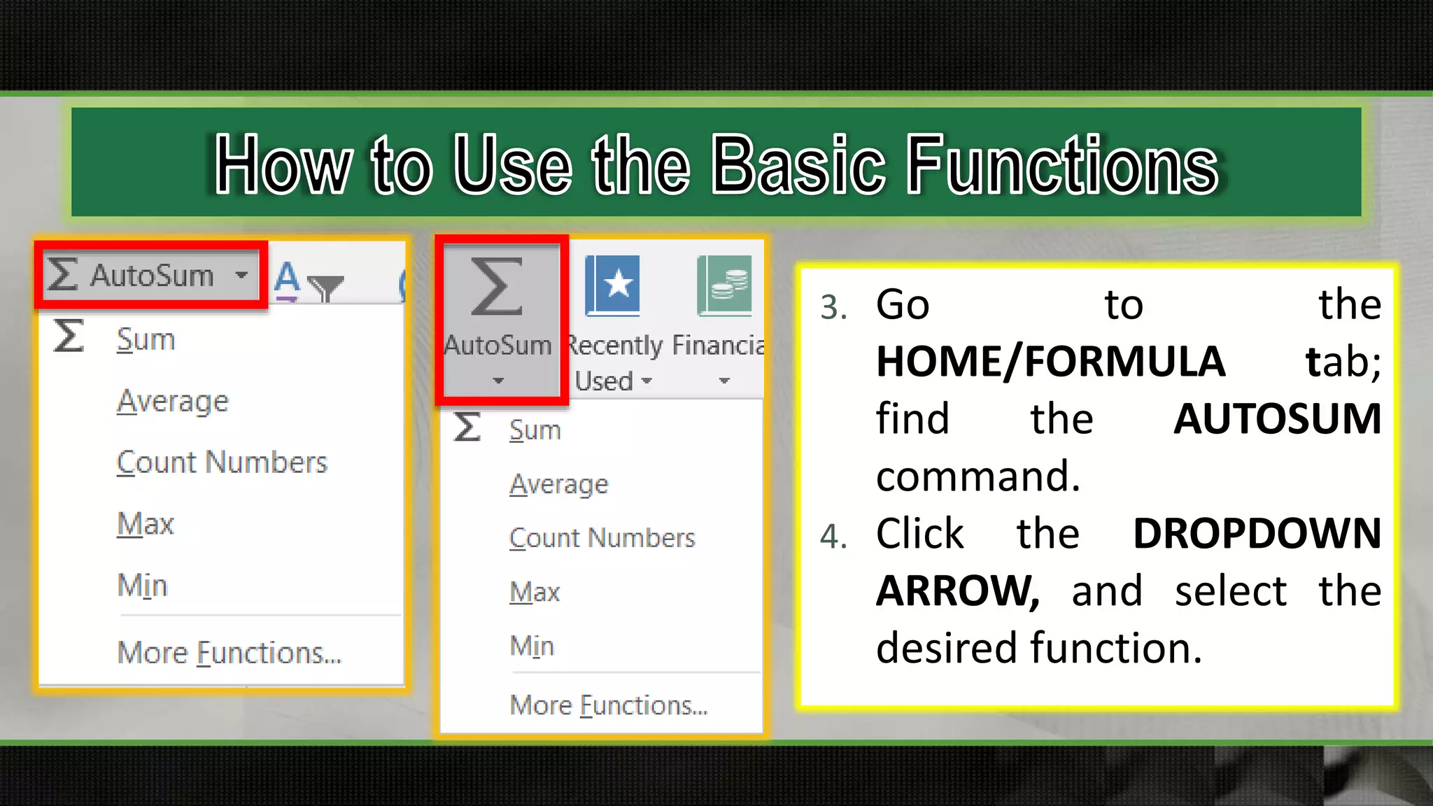
3. Go to the HOME/FORMULA tab, find the
AUTOSUM Command.
4. Click the dropdown arrow and select the
desired function.
20.
1. Create thetable with rows & columns of data.
2. Select all the desired cells.
21.
3. Go tothe
HOME/FORMULA tab;
find the AUTOSUM
command.
4. Click the DROPDOWN
ARROW, and select the
desired function.
23.
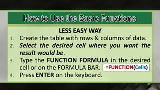
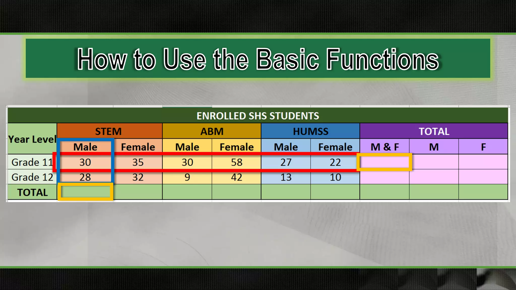
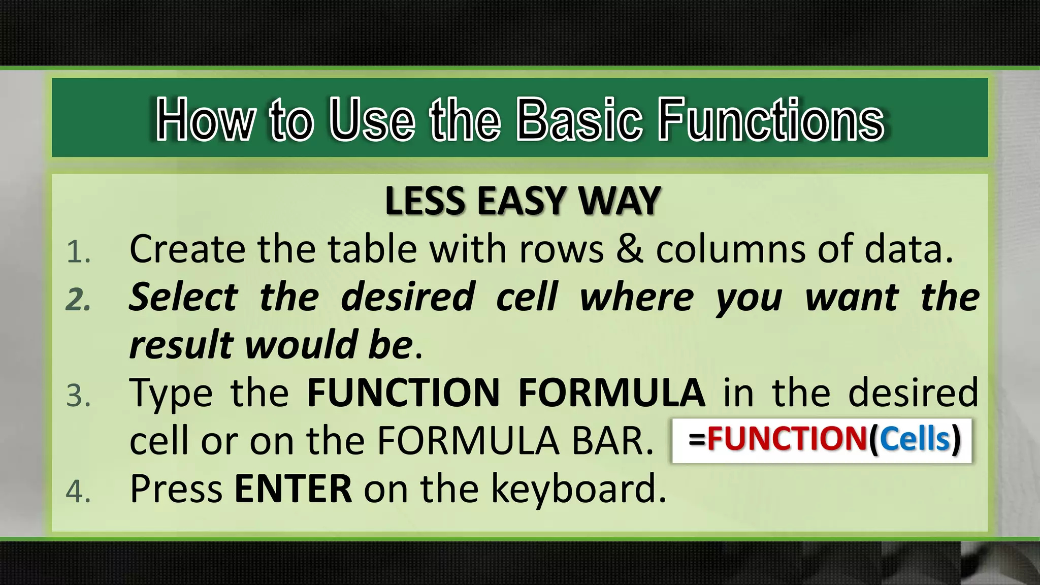
LESS EASY WAY
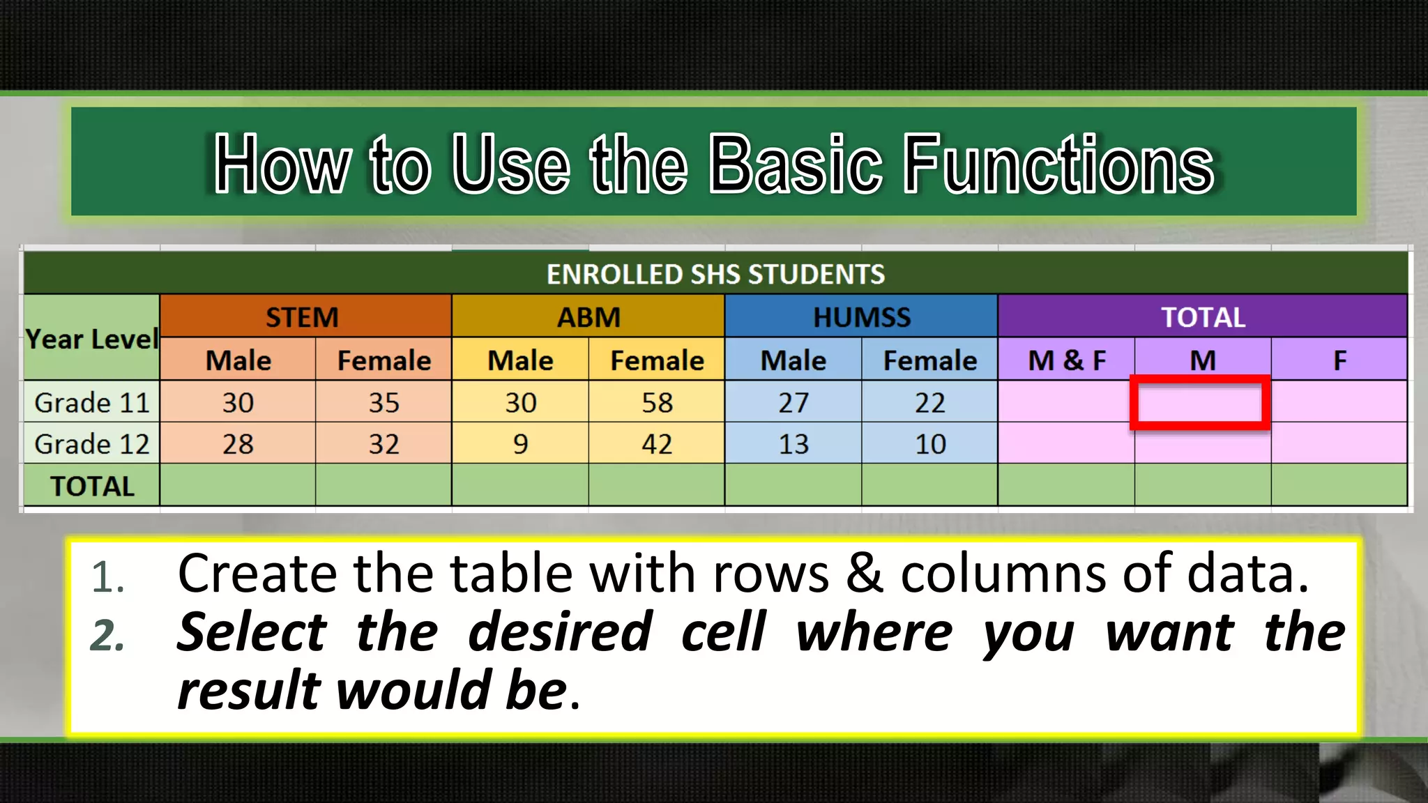
1.Create the table with rows & columns of data.
2. Select the desired cell where you want the
result would be.
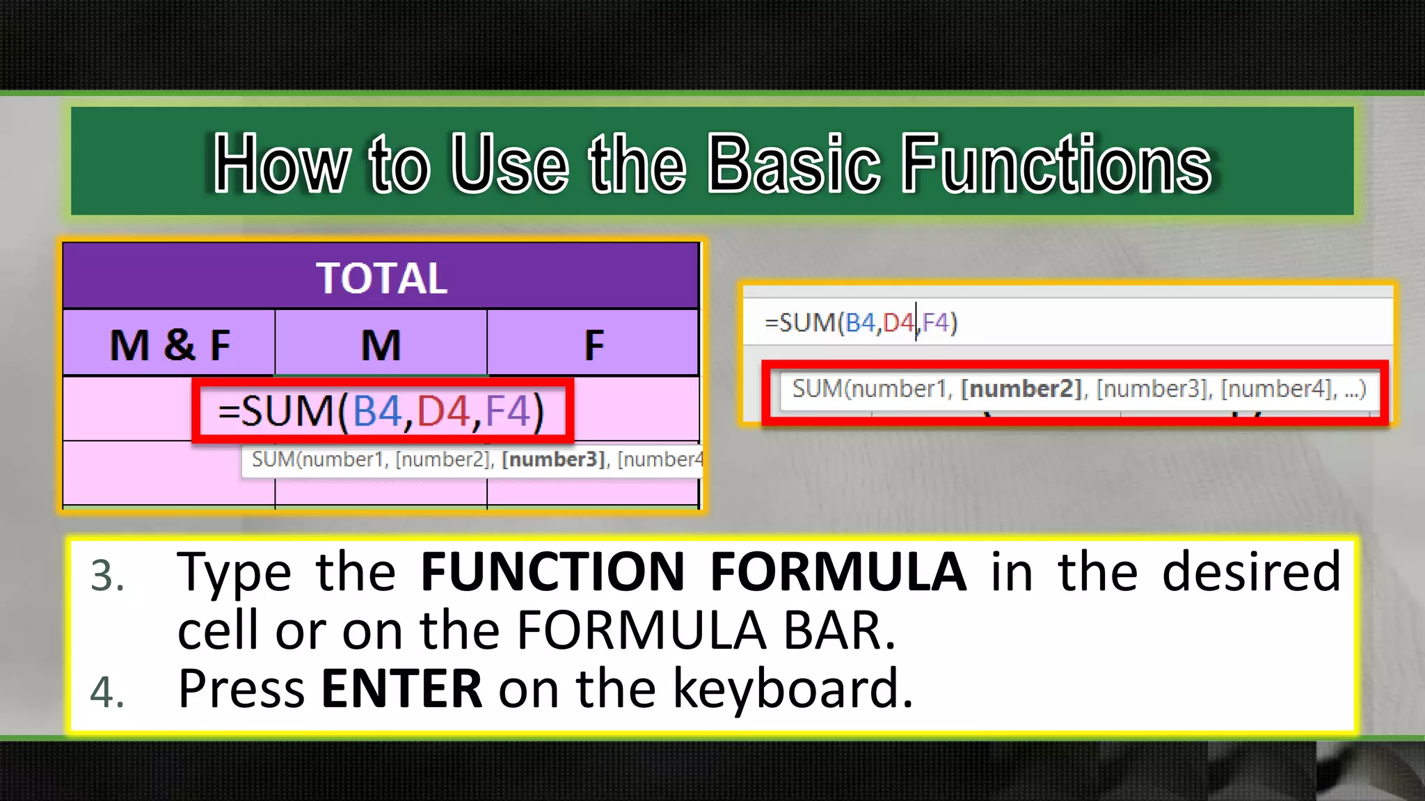
3. Type the FUNCTION FORMULA in the desired
cell or on the FORMULA BAR.
4. Press ENTER on the keyboard.
=FUNCTION(Cells)
24.
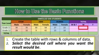
1. Create thetable with rows & columns of data.
2. Select the desired cell where you want the
result would be.
25.
3. Type theFUNCTION FORMULA in the desired
cell or on the FORMULA BAR.
4. Press ENTER on the keyboard.
26.
FUNCTION FORMULA
Sum =SUM()
Average =AVERAGE( )
Max =MAX( )
Min =MIN( )
FUNCTION FORMULA
Count =COUNT( )
CountA =COUNTA( )
Concatenate =CONCAT( )
Round =ROUND( )
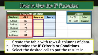
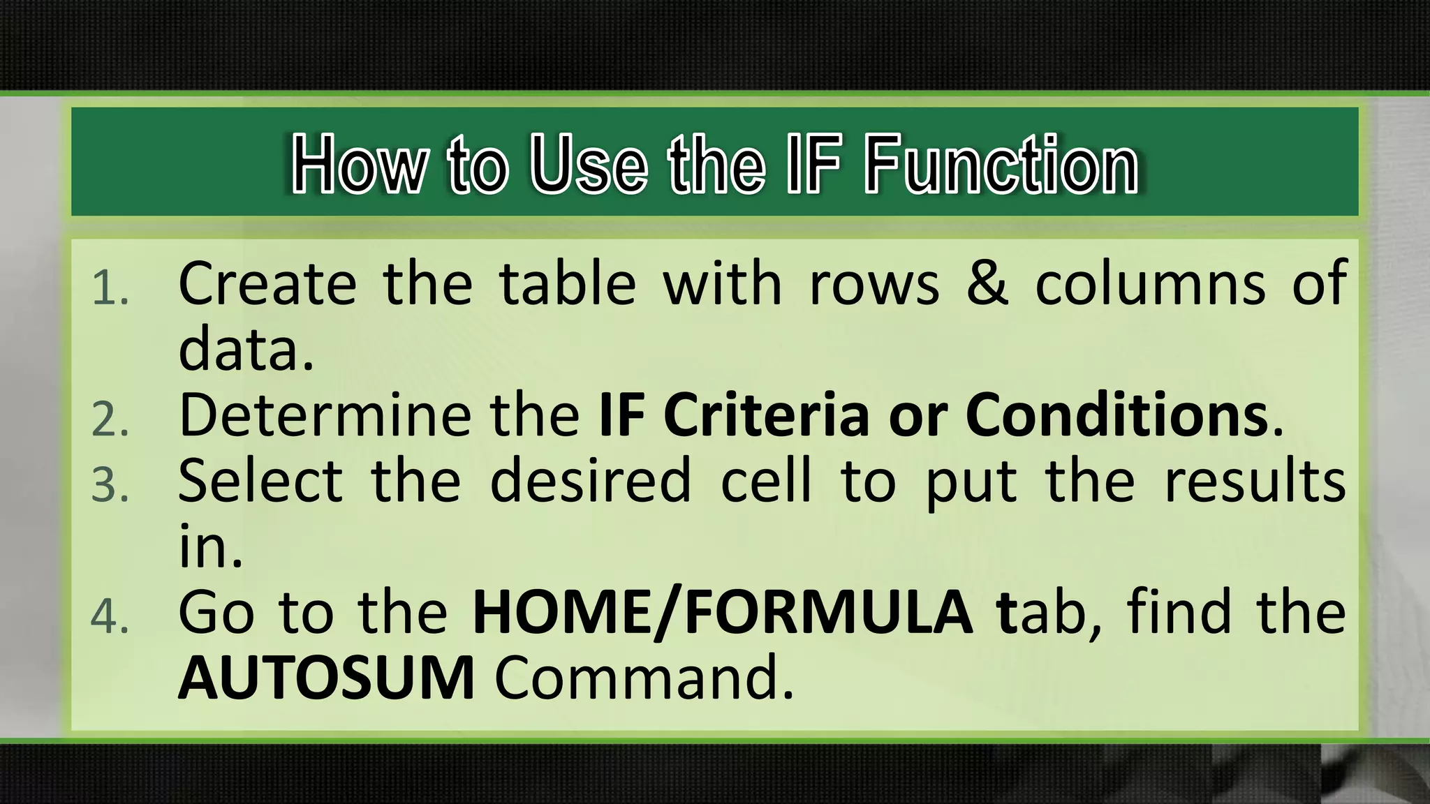
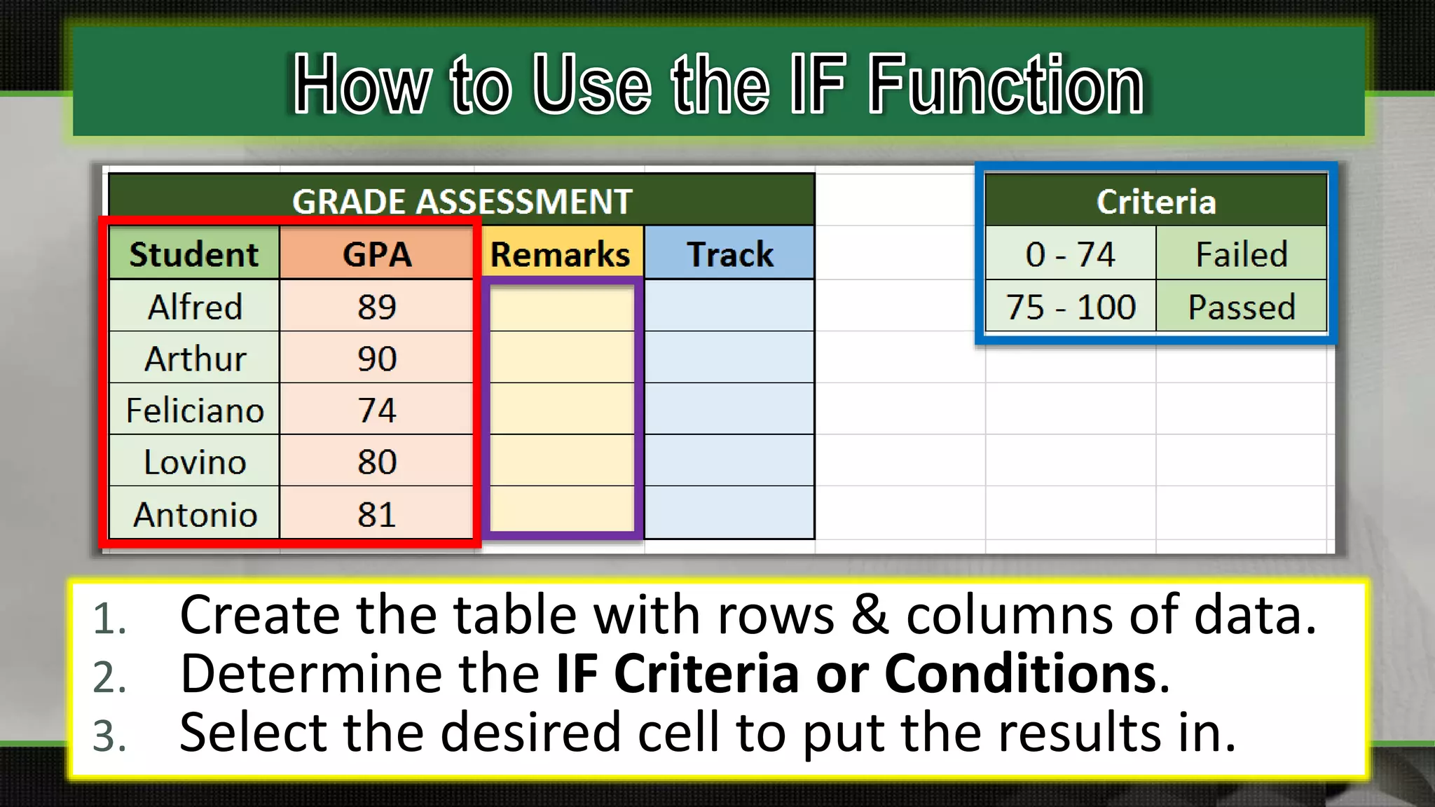
1. Create thetable with rows & columns of
data.
2. Determine the IF Criteria or Conditions.
3. Select the desired cell to put the results
in.
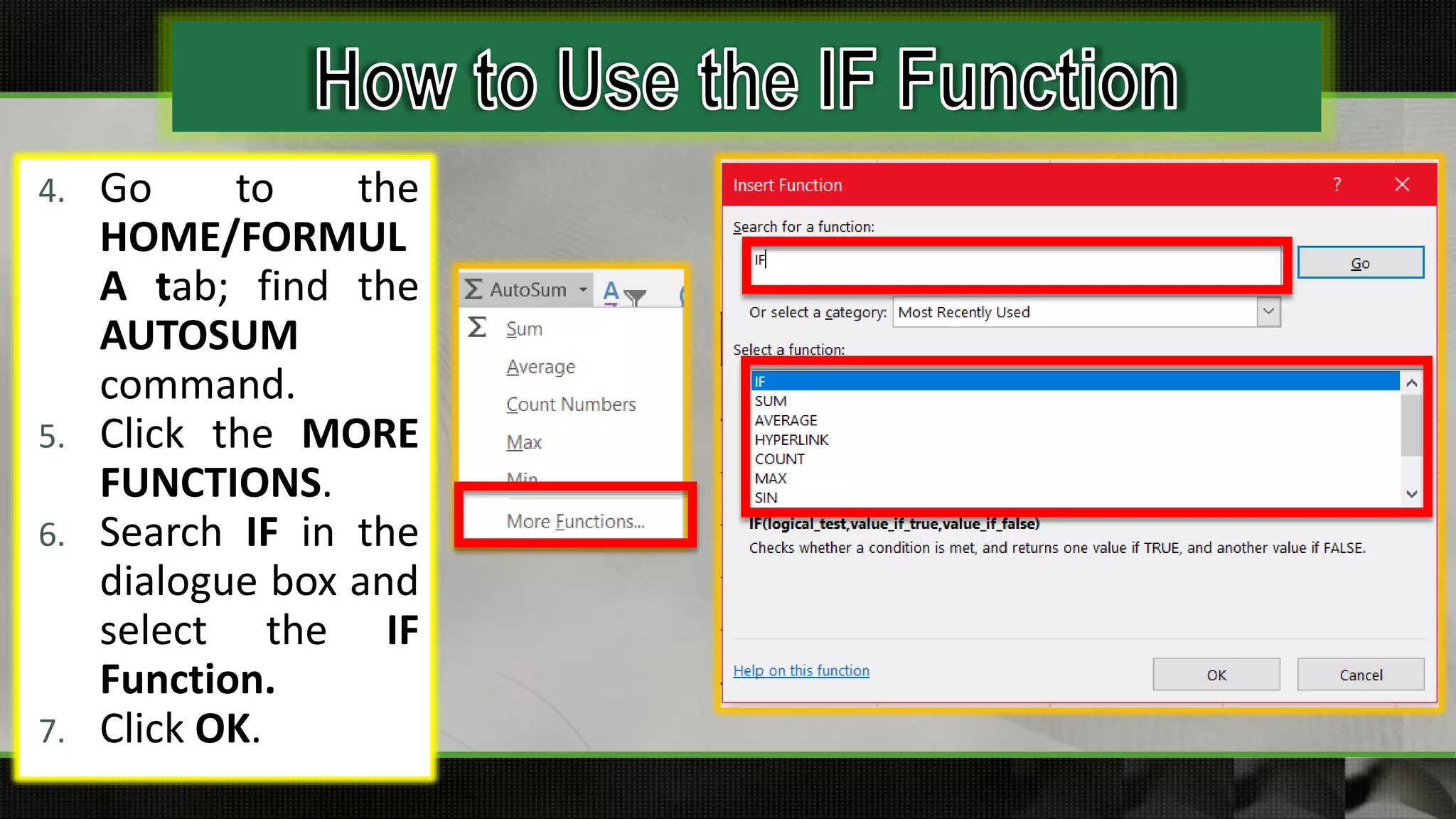
4. Go to the HOME/FORMULA tab, find the
AUTOSUM Command.
29.
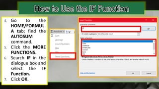
5. Click theMORE FUNCTIONS.
6. Search IF in the dialogue box and
select the IF Function.
7. Click OK.
30.
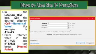
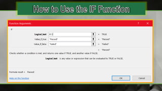
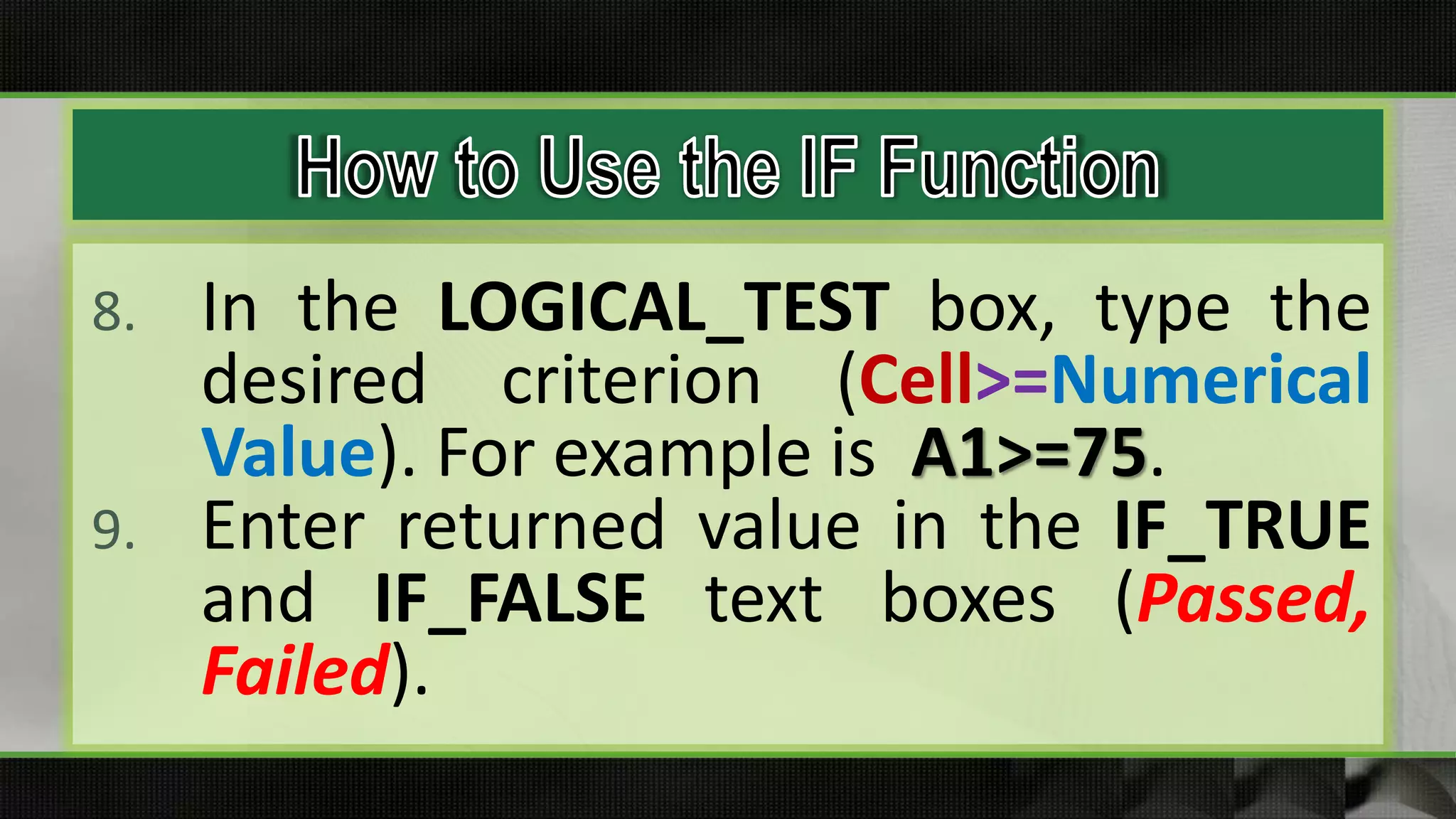
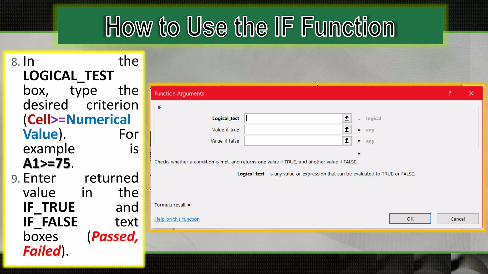
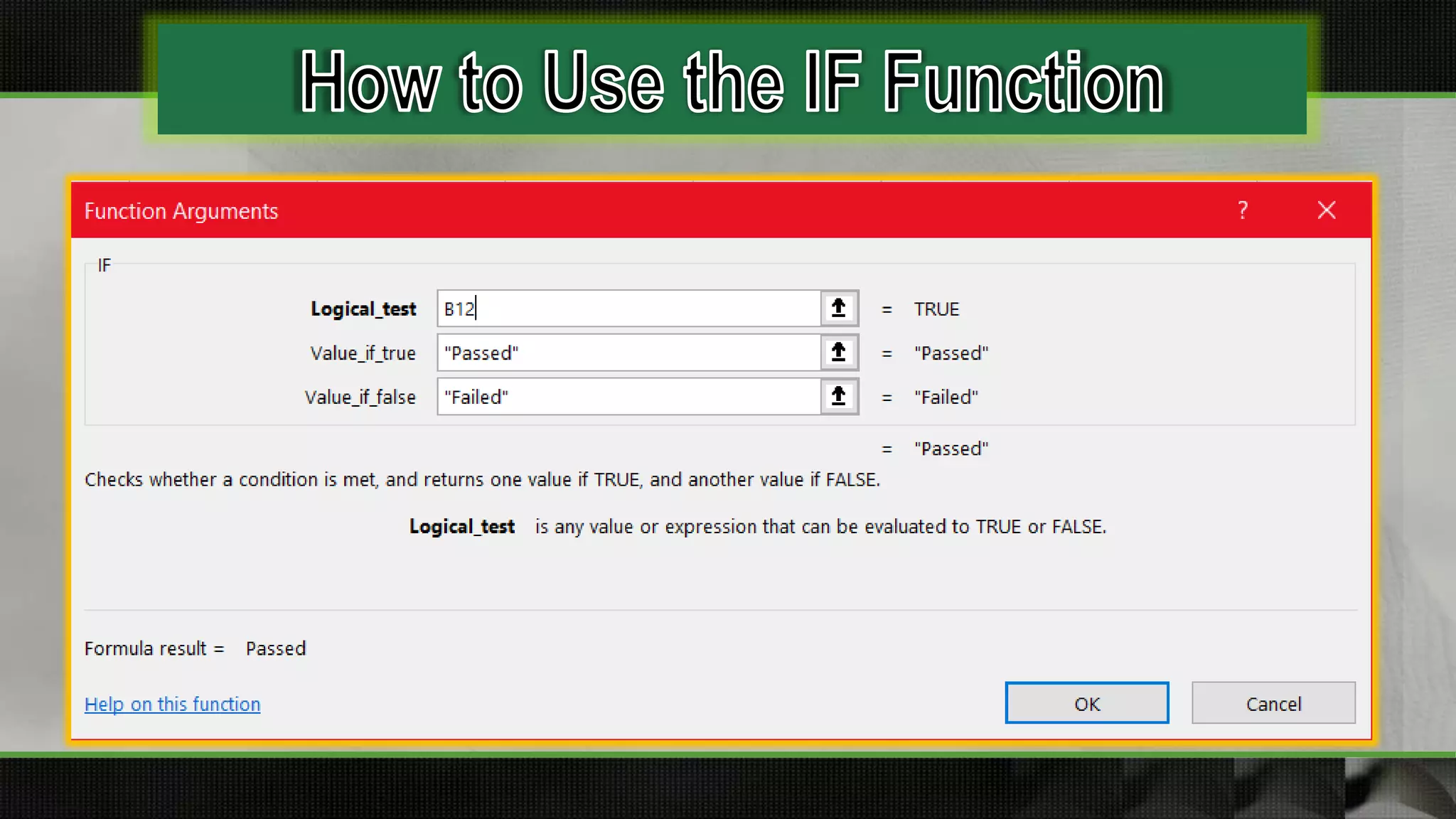
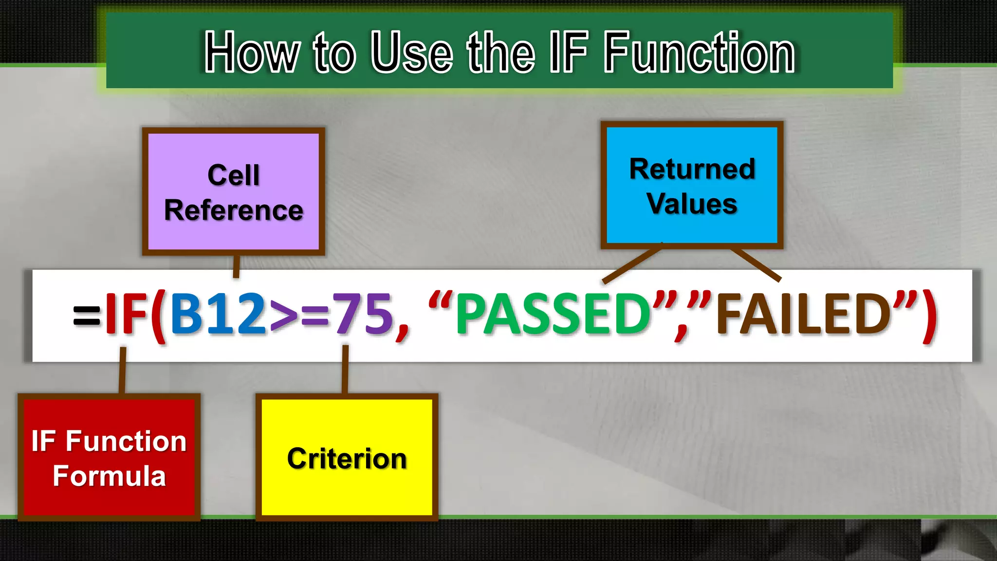
8. In theLOGICAL_TEST box, type the
desired criterion (Cell>=Numerical
Value). For example is A1>=75.
9. Enter returned value in the IF_TRUE
and IF_FALSE text boxes (Passed,
Failed).
31.
1. Create thetable with rows & columns of data.
2. Determine the IF Criteria or Conditions.
3. Select the desired cell to put the results in.
32.
4. Go tothe
HOME/FORMUL
A tab; find the
AUTOSUM
command.
5. Click the MORE
FUNCTIONS.
6. Search IF in the
dialogue box and
select the IF
Function.
7. Click OK.
33.
8. In the
LOGICAL_TEST
box,type the
desired criterion
(Cell>=Numerical
Value). For
example is
A1>=75.
9. Enter returned
value in the
IF_TRUE and
IF_FALSE text
boxes (Passed,
Failed).
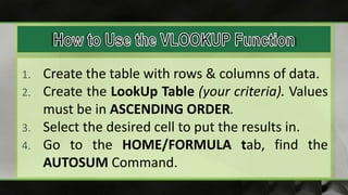
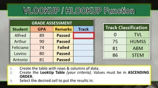
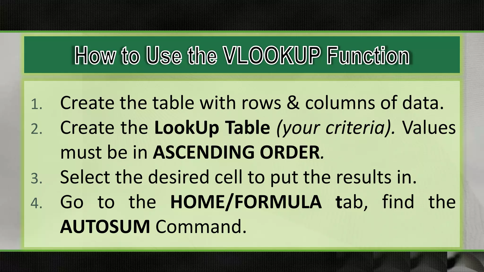
1. Create thetable with rows & columns of data.
2. Create the LookUp Table (your criteria). Values
must be in ASCENDING ORDER.
3. Select the desired cell to put the results in.
4. Go to the HOME/FORMULA tab, find the
AUTOSUM Command.
39.
5. Click theMORE FUNCTIONS.
6. Search VLOOKUP in the dialogue
box and select the function.
7. Click OK.
40.
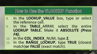
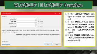
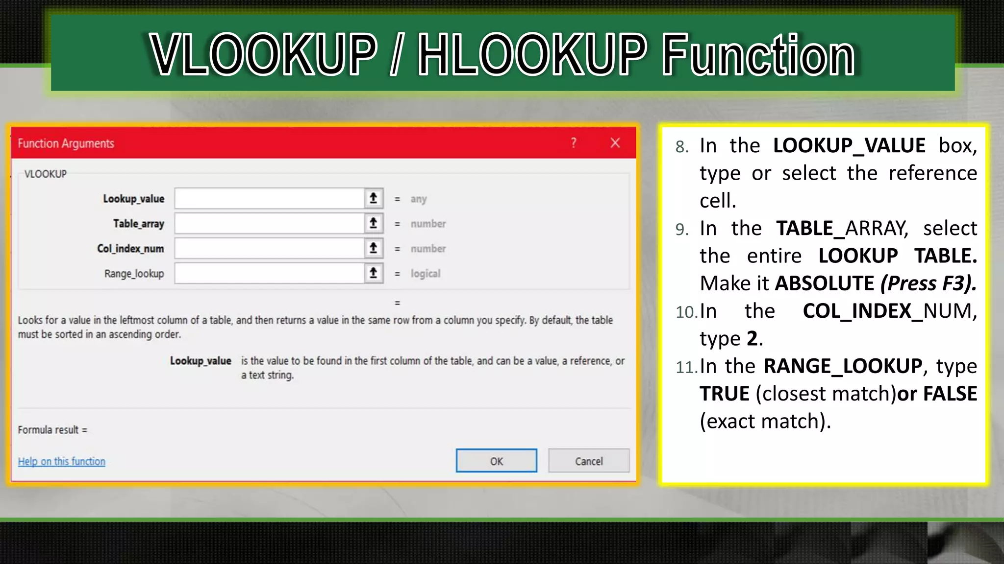
8. In theLOOKUP_VALUE box, type or select
the reference cell.
9. In the TABLE_ARRAY, select the entire
LOOKUP TABLE. Make it ABSOLUTE (Press
F4).
10. In the COL_INDEX_NUM, type 2.
11. In the RANGE_LOOKUP, type TRUE (closest
match)or FALSE (exact match).
41.
1. Create thetable with rows & columns of data.
2. Create the LookUp Table (your criteria). Values must be in ASCENDING
ORDER.
3. Select the desired cell to put the results in.
42.
8. In theLOOKUP_VALUE box,
type or select the reference
cell.
9. In the TABLE_ARRAY, select
the entire LOOKUP TABLE.
Make it ABSOLUTE (Press F3).
10.In the COL_INDEX_NUM,
type 2.
11.In the RANGE_LOOKUP, type
TRUE (closest match)or FALSE
(exact match).
43.
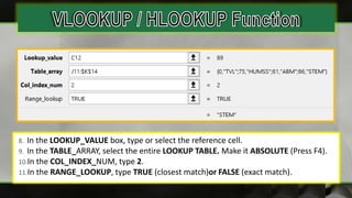
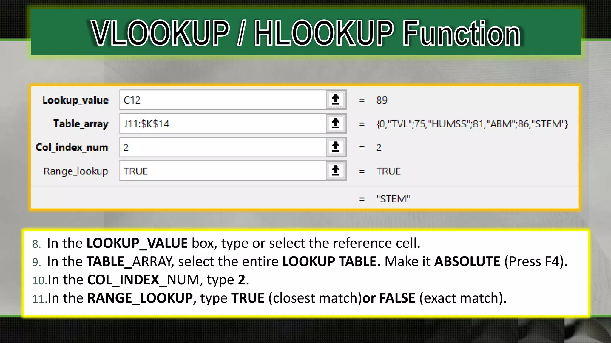
8. In theLOOKUP_VALUE box, type or select the reference cell.
9. In the TABLE_ARRAY, select the entire LOOKUP TABLE. Make it ABSOLUTE (Press F4).
10.In the COL_INDEX_NUM, type 2.
11.In the RANGE_LOOKUP, type TRUE (closest match)or FALSE (exact match).


![Etech. mitch. [autosaved]](https://cdn.slidesharecdn.com/ss_thumbnails/etech-190128010709-thumbnail.jpg?width=600ounds&width=560&fit=bounds)


