Downloaded 1,048 times
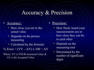
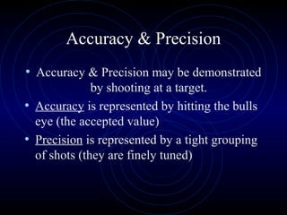
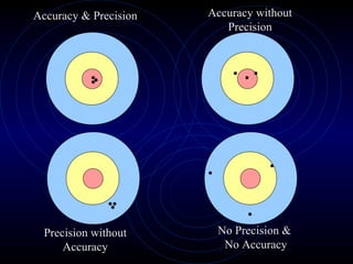
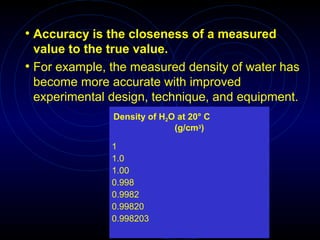
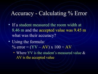
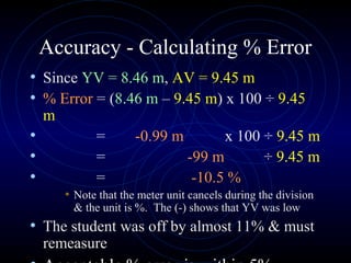
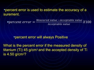


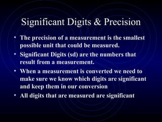

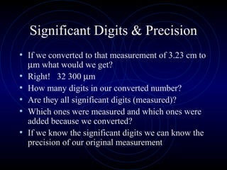
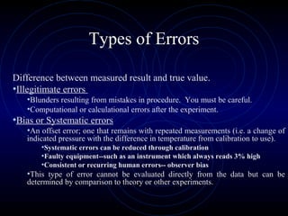
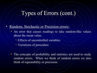
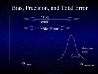

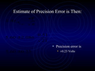
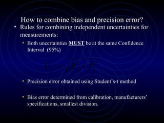
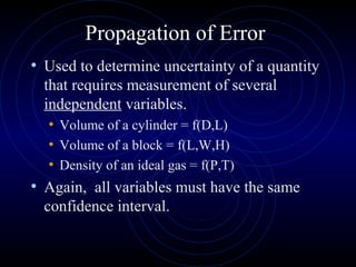
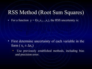
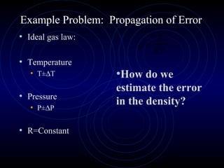
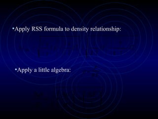

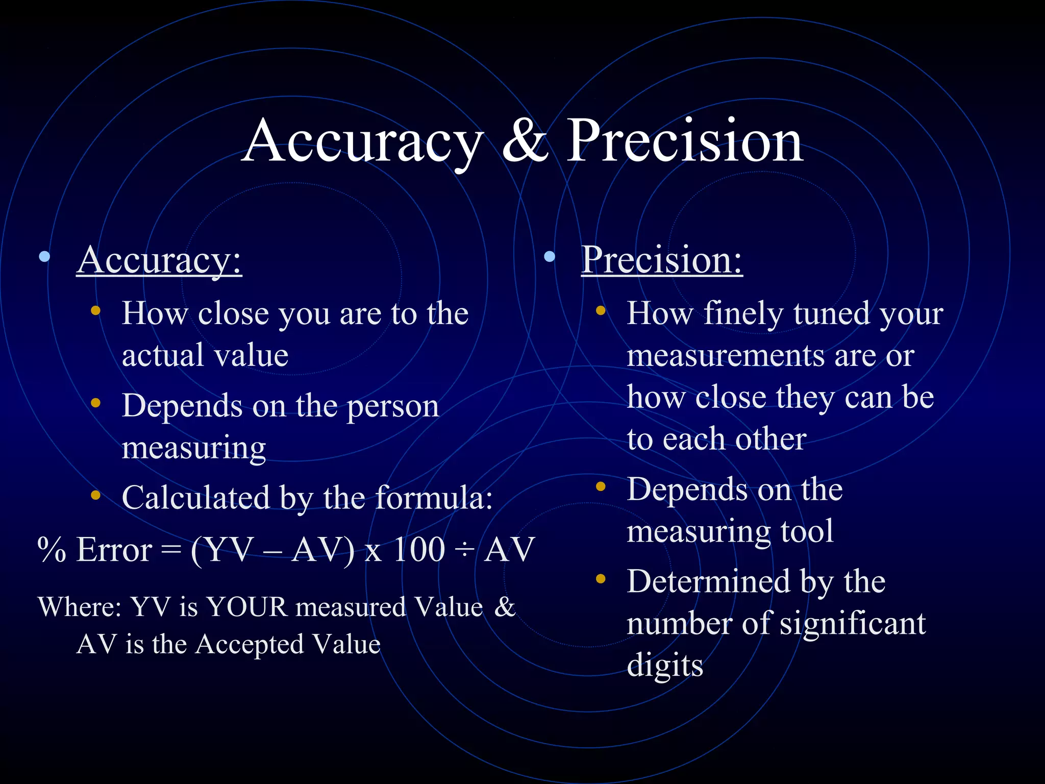
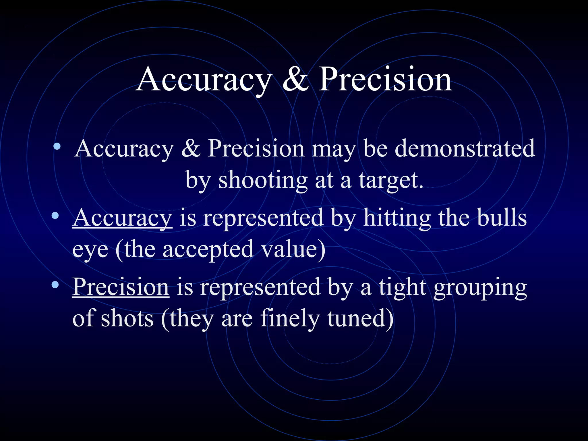
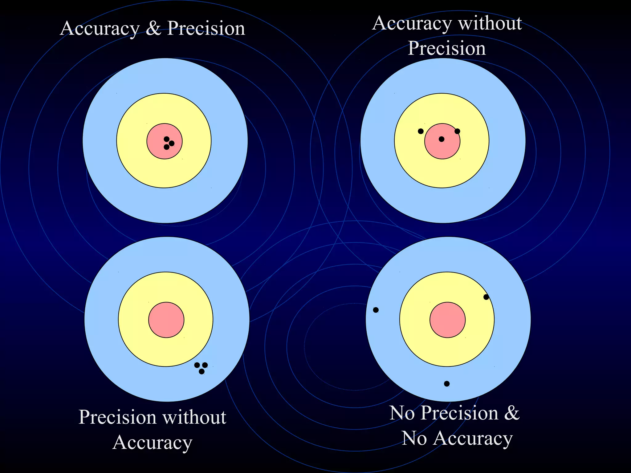
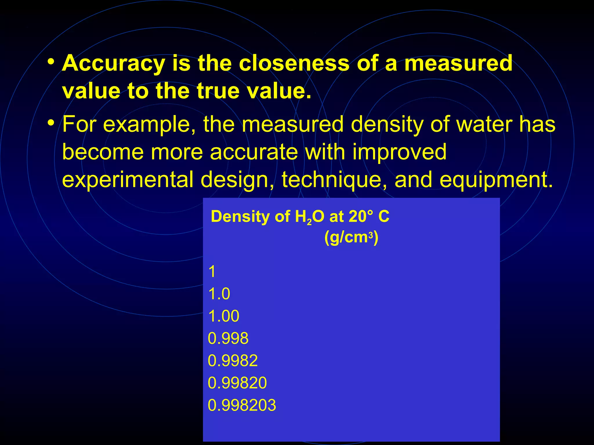
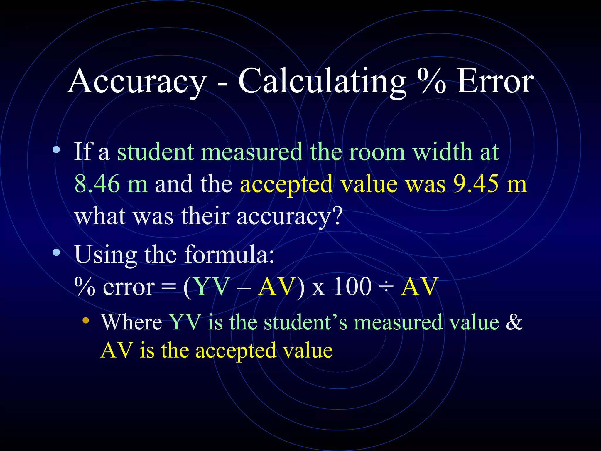
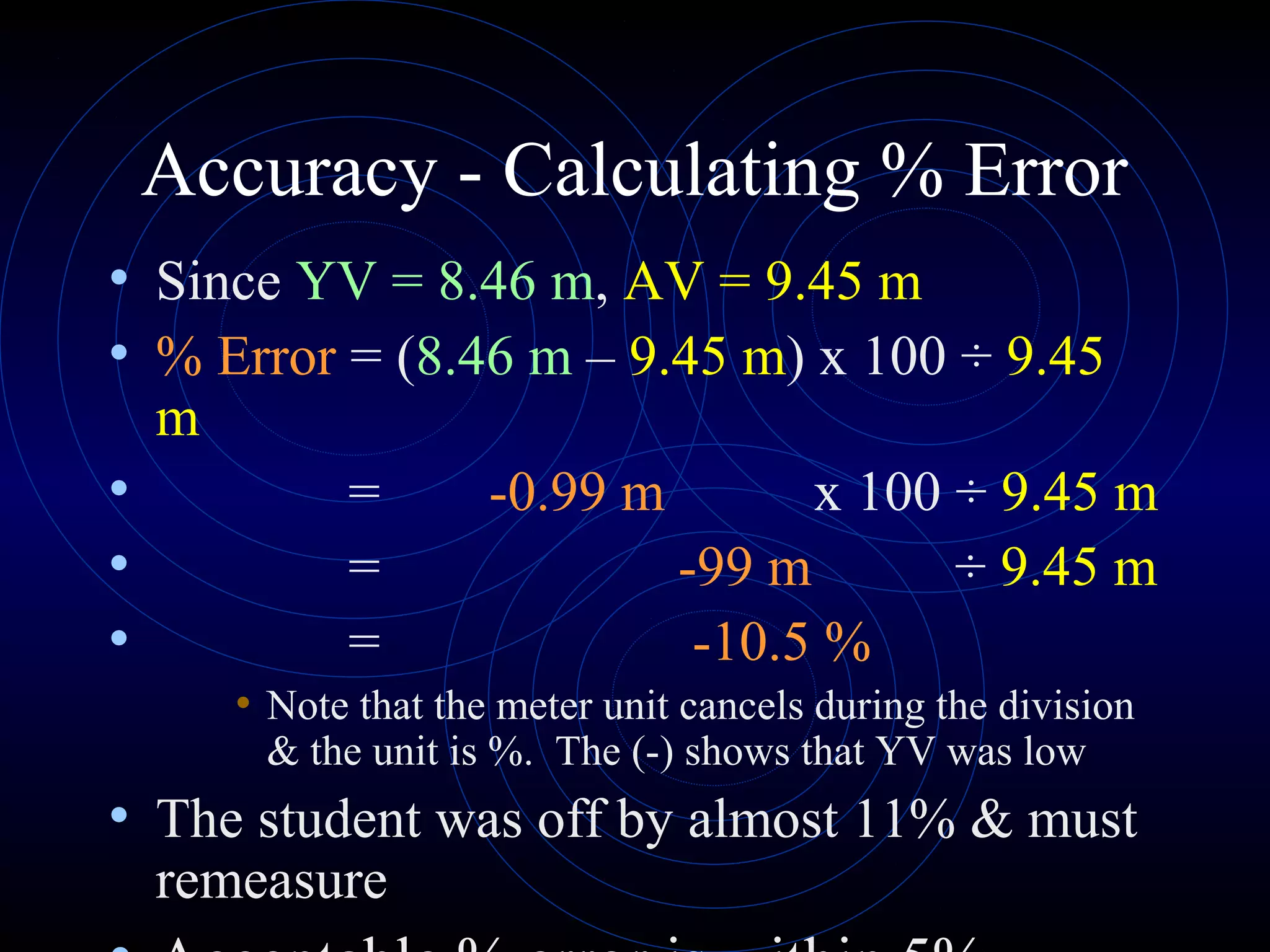
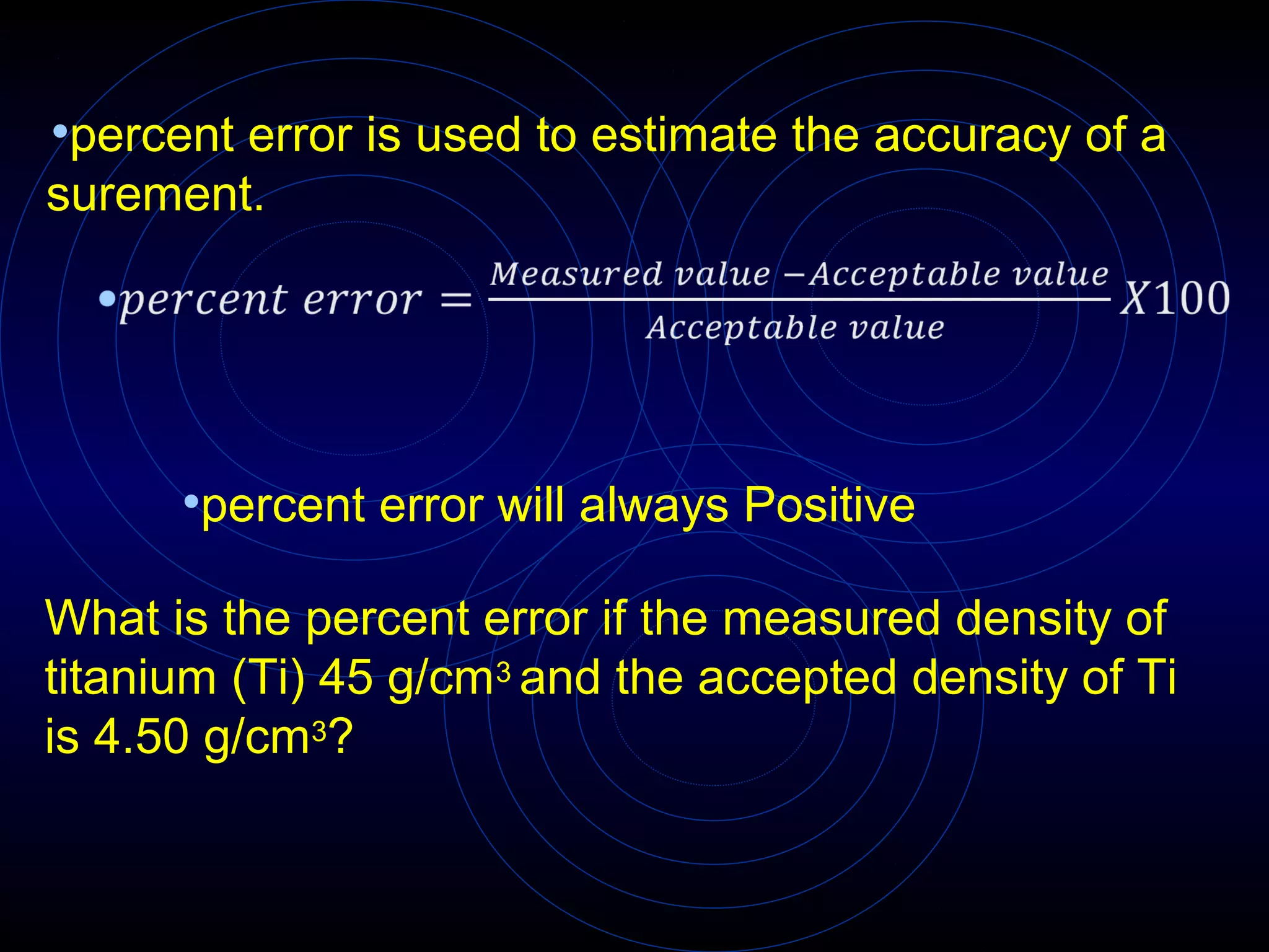
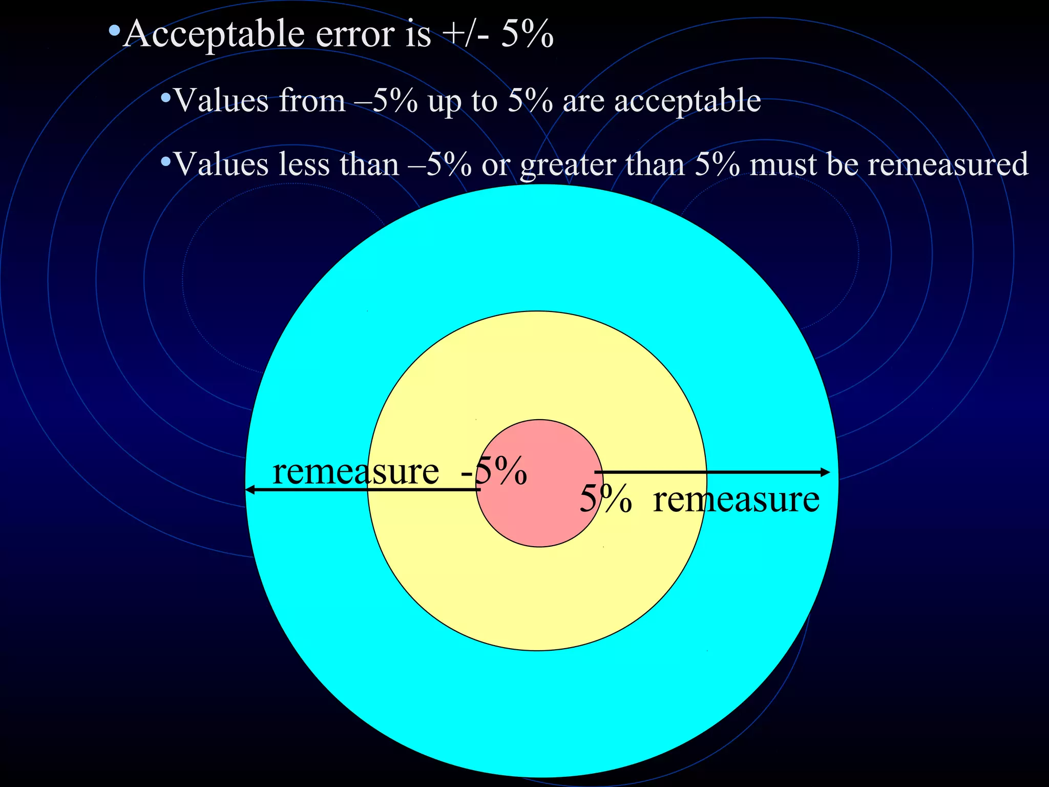

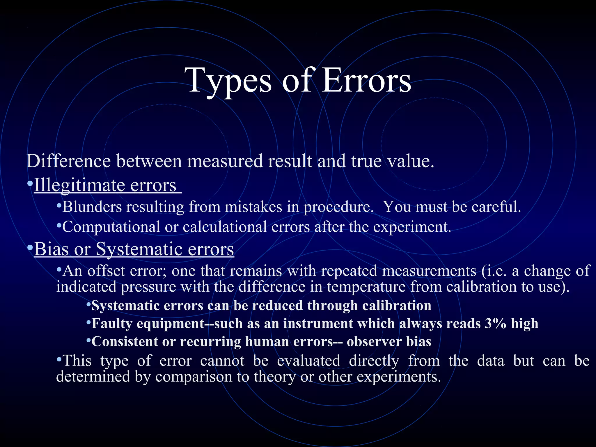
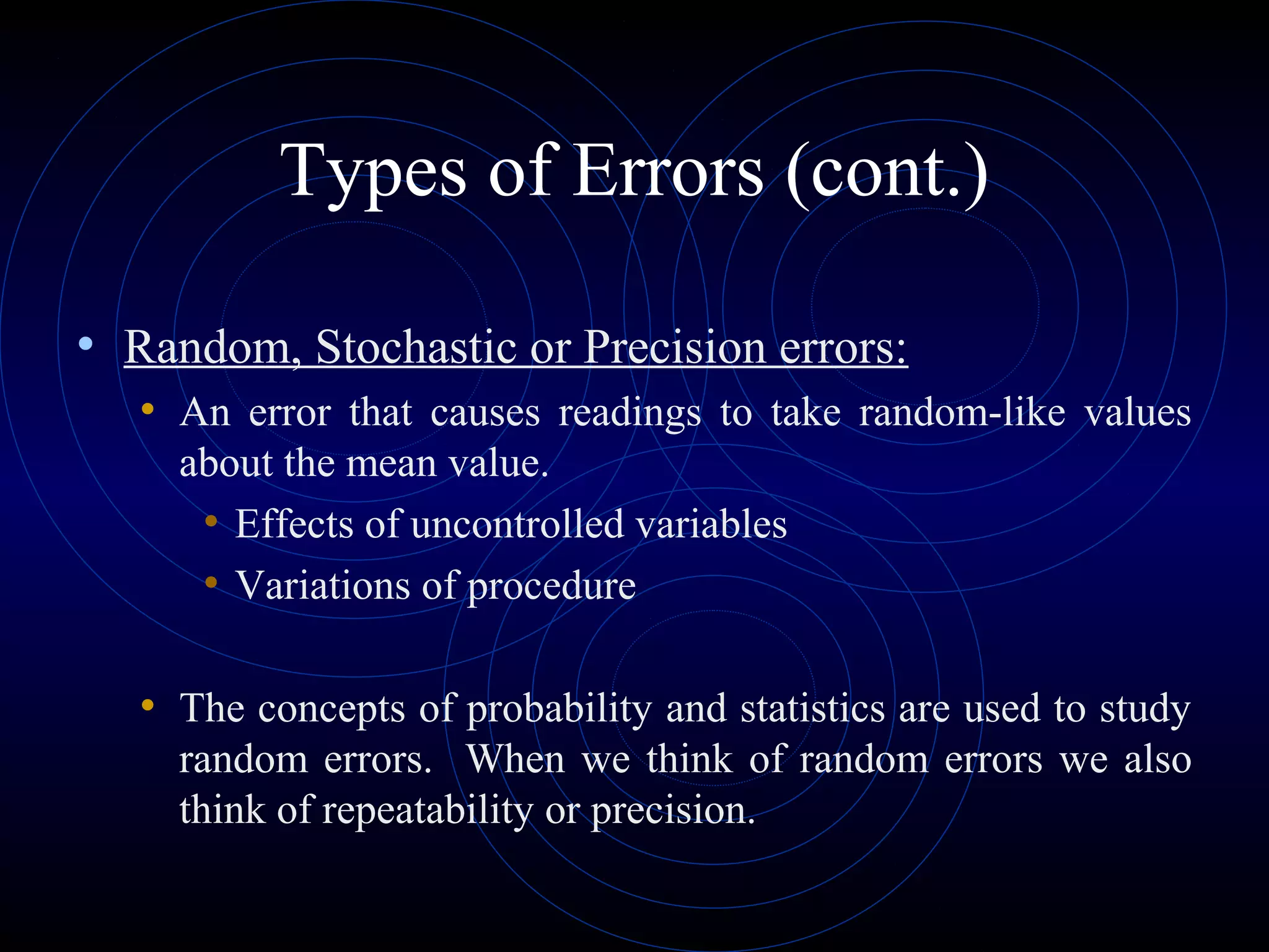
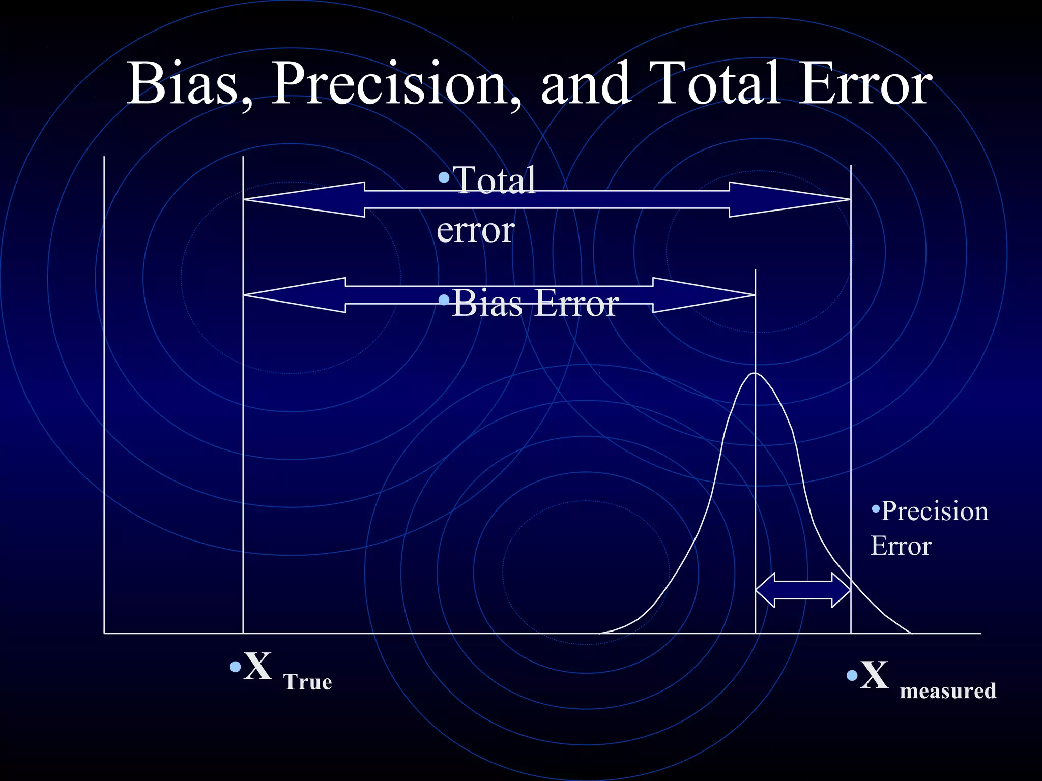
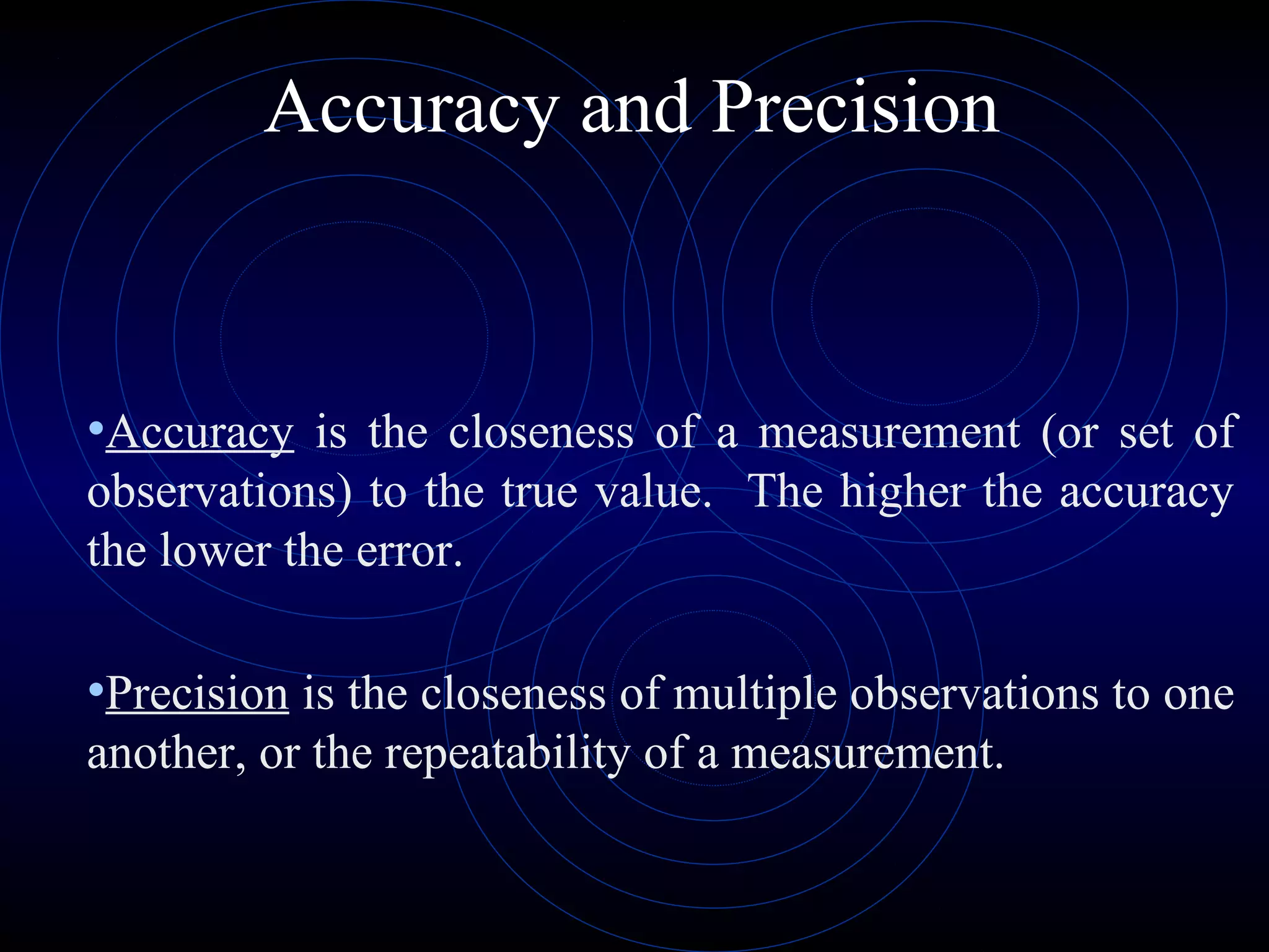


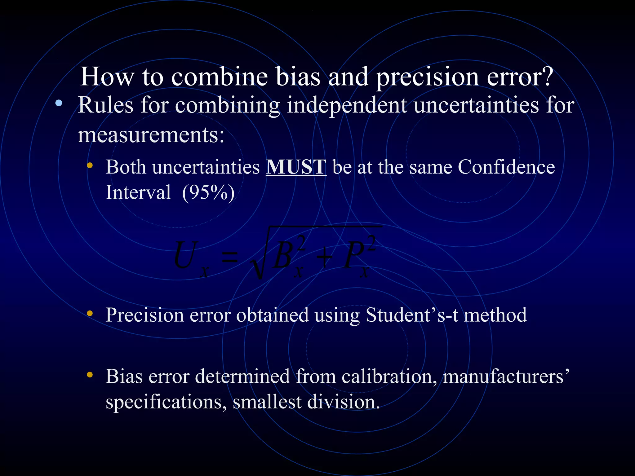

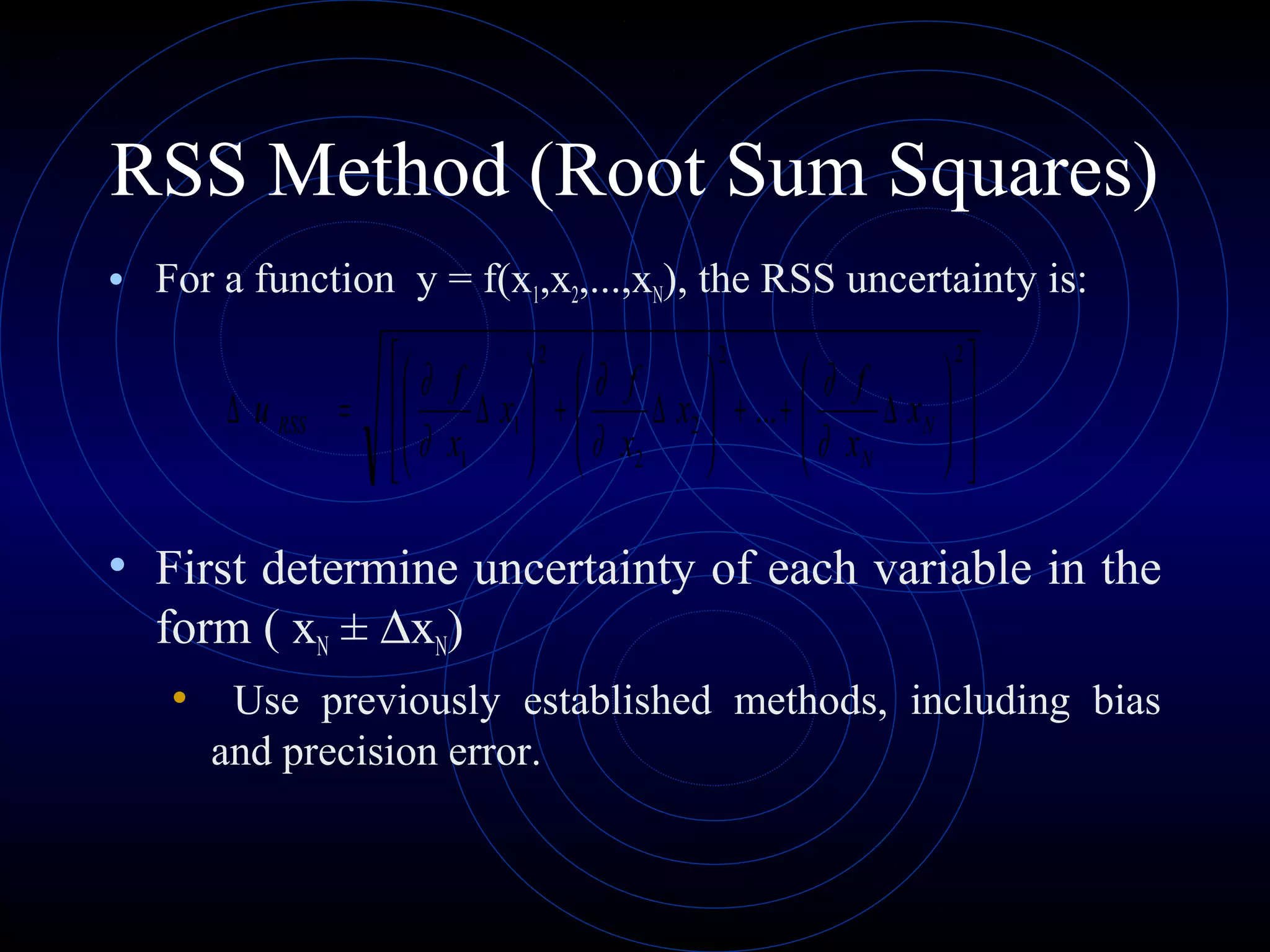


Accuracy refers to how close a measurement is to the true value, while precision refers to the reproducibility of measurements. Accuracy is determined by calculating percentage error compared to the accepted value. Precision depends on the number of significant figures in a measurement as determined by the measuring tool. Random and systematic errors can affect accuracy, while random errors affect precision. The uncertainty of a measurement combines its precision and accuracy errors and is reported with the mean value and at a given confidence level, typically 95%. Propagation of error calculations allow determining the total uncertainty when a value depends on multiple measurements.


