N. V. RATNAKISHORGADE 1
Solving Problems by
Searching
ARTIFICIAL INTELLIGENCE : A MODERN APPROACH, STUART J.
RUSSELL AND PETER NORVIG, 3RD
EDITION, PRENTICE HALL
2.
N. V. RATNAKISHORGADE 2
Problem-Solving Agents
Kind of goal-based agents.
Uses the atomic representations Each state of the environment is
indivisible and has no internal structure visible to the problem solving algorithm.
Steps in problem – solving
1. Goal Formulation
2. Problem Formulation
3. Search
4. Execution
3.
N. V. RATNAKISHORGADE 3
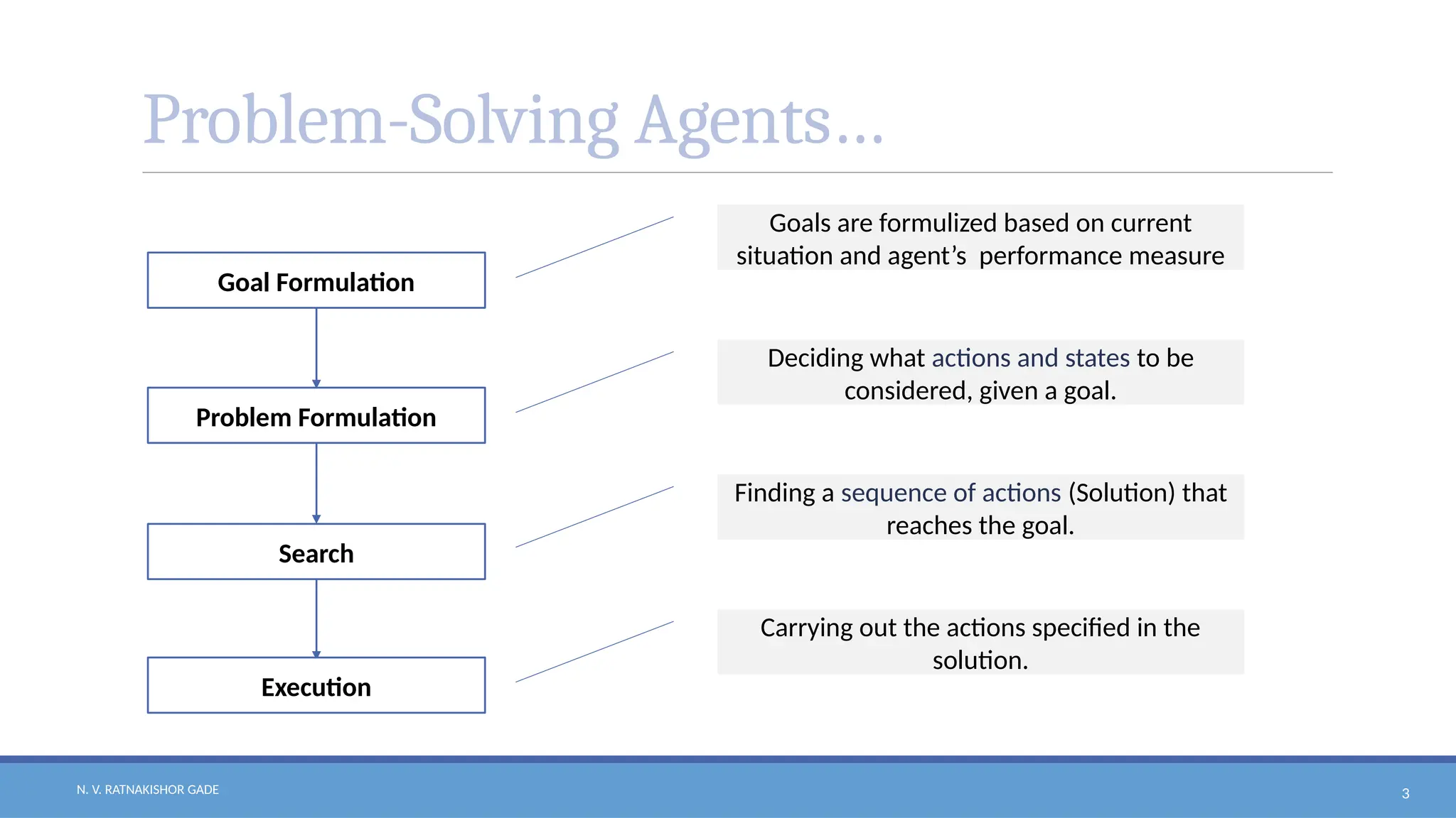
Problem-Solving Agents…
Goal Formulation
Problem Formulation
Search
Execution
Goals are formulized based on current
situation and agent’s performance measure
Deciding what actions and states to be
considered, given a goal.
Finding a sequence of actions (Solution) that
reaches the goal.
Carrying out the actions specified in the
solution.
4.
N. V. RATNAKISHORGADE 4
Problem-Solving Agents…
Pseudo code for Simple Problem – Solving Agent:
action_sequence = [] # Action Sequence, initially empty
goal = null # Goal, initially Null
function Simple_Problem_Solving_Agent(percept) returns action:
state = UPDATE_STATE(state, percept) # State Update
if action_sequence is empty then:
goal = FORMULATE_GOAL(state) # Goal Formulation
problem = FORMULATE_PROBLEM(state, goal) # Problem Formulation
action_sequence = SEARCH(problem) # Searching to find the solution
action = FIRST(action_sequence) # Discharge action for execution
action_sequence = REST(action_sequence) # Remove the discharged action from action sequence
return action
5.
N. V. RATNAKISHORGADE 5
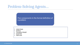
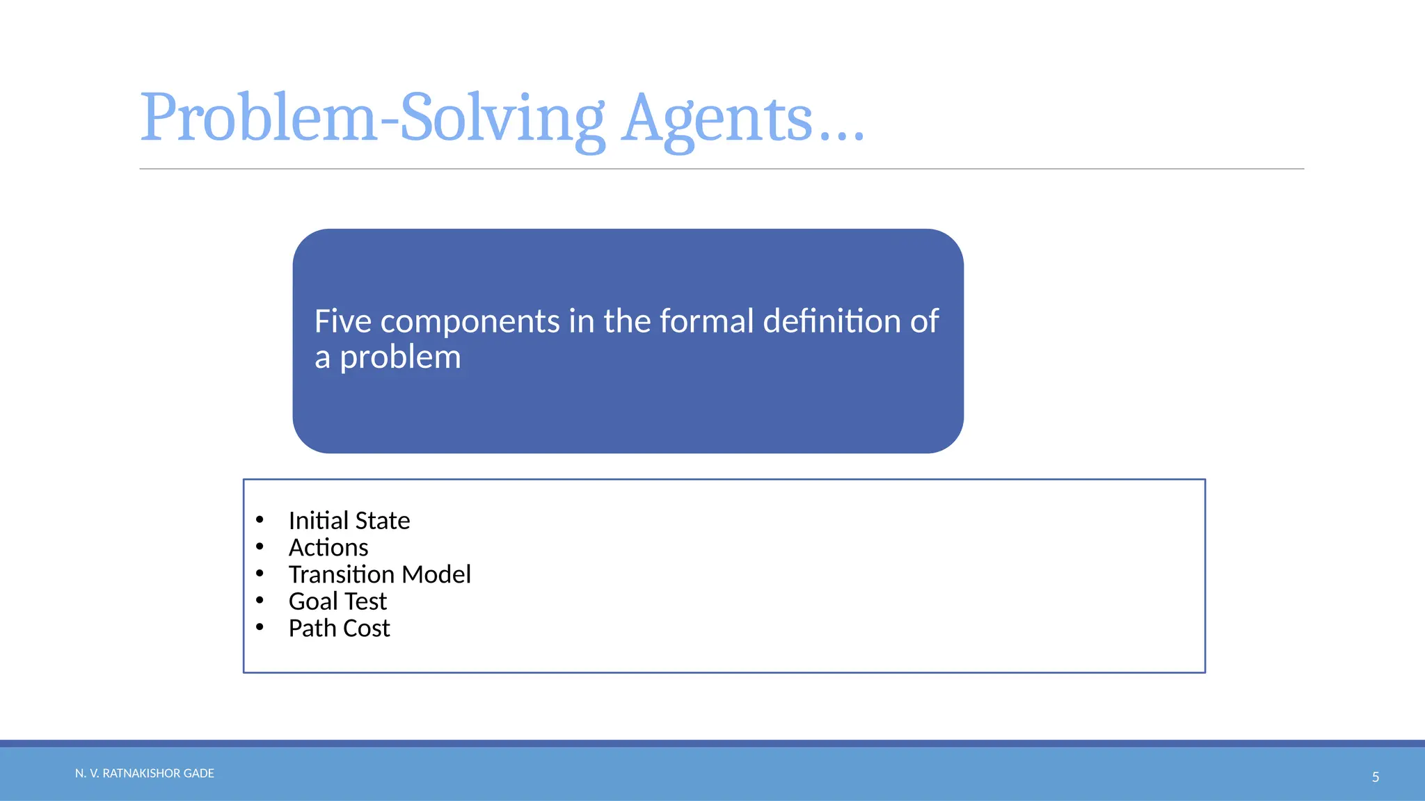
Problem-Solving Agents…
Five components in the formal definition of
a problem
• Initial State
• Actions
• Transition Model
• Goal Test
• Path Cost
6.
N. V. RATNAKISHORGADE 6
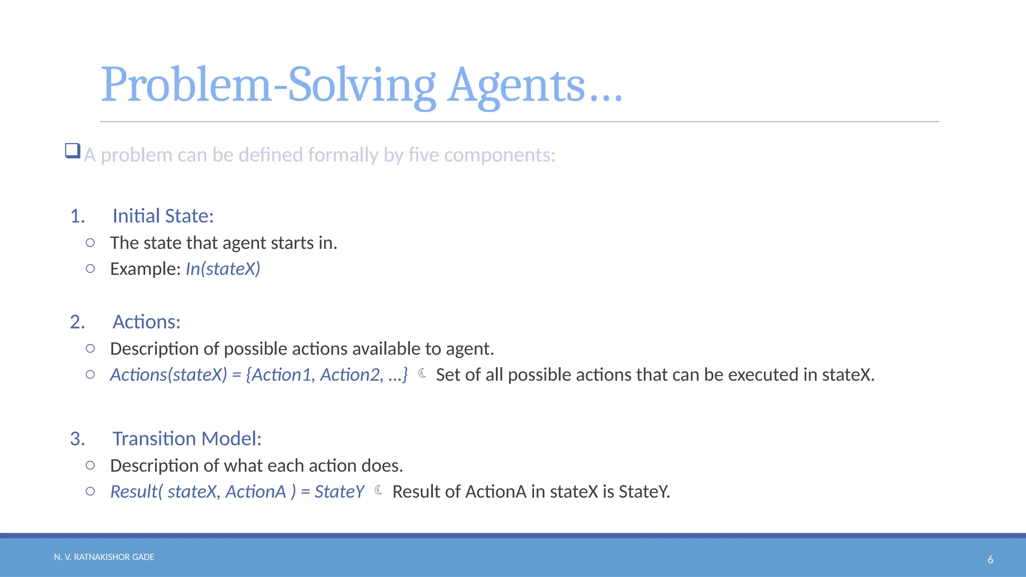
Problem-Solving Agents…
A problem can be defined formally by five components:
1. Initial State:
o The state that agent starts in.
o Example: In(stateX)
2. Actions:
o Description of possible actions available to agent.
o Actions(stateX) = {Action1, Action2, …} Set of all possible actions that can be executed in stateX.
3. Transition Model:
o Description of what each action does.
o Result( stateX, ActionA ) = StateY Result of ActionA in stateX is StateY.
7.
N. V. RATNAKISHORGADE 7
Problem-Solving Agents…
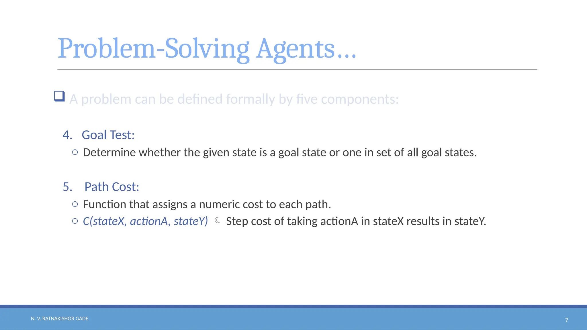
A problem can be defined formally by five components:
4. Goal Test:
o Determine whether the given state is a goal state or one in set of all goal states.
5. Path Cost:
o Function that assigns a numeric cost to each path.
o C(stateX, actionA, stateY) Step cost of taking actionA in stateX results in stateY.
8.
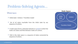
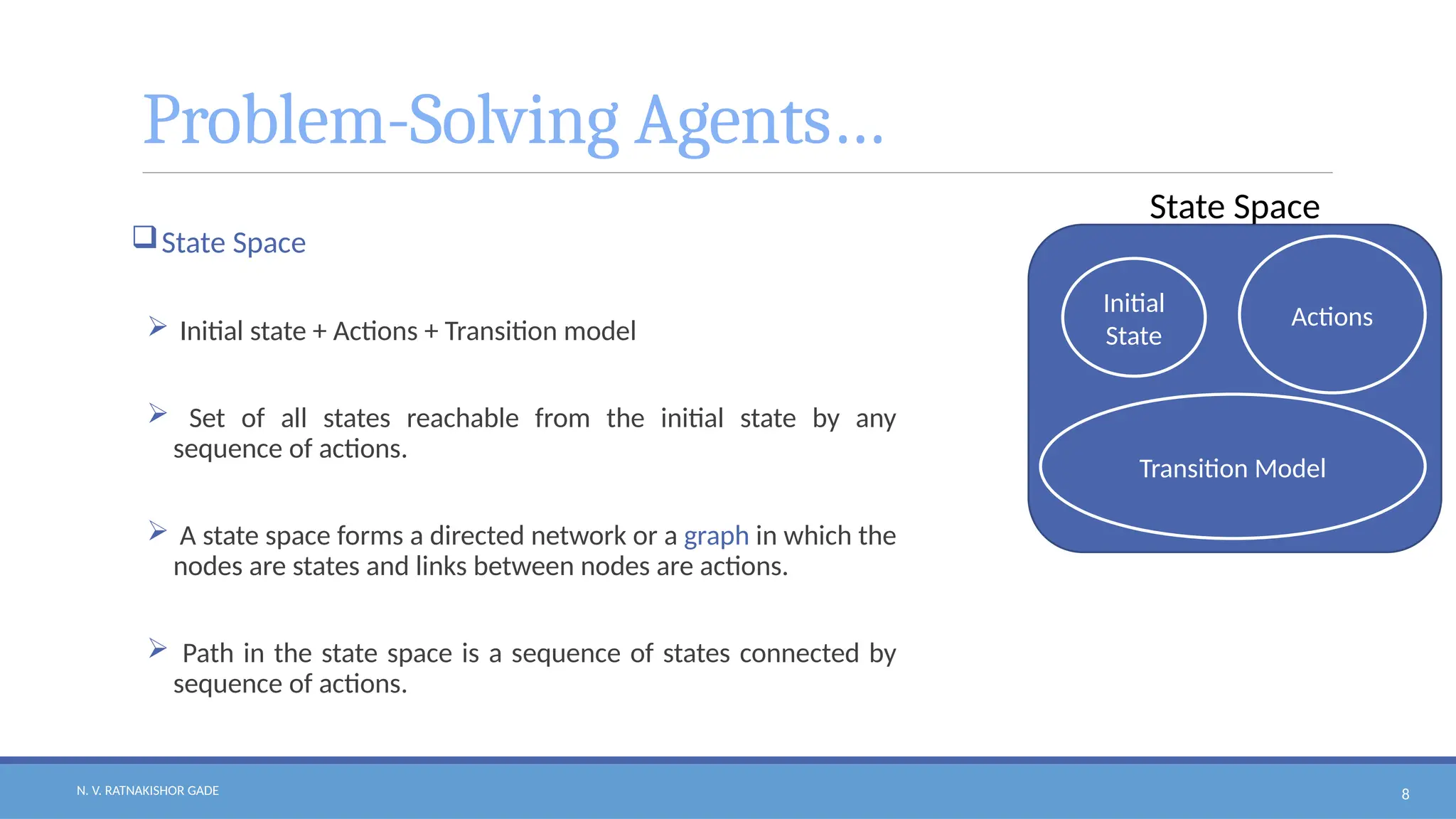
N. V. RATNAKISHORGADE 8
Problem-Solving Agents…
State Space
Initial state + Actions + Transition model
Set of all states reachable from the initial state by any
sequence of actions.
A state space forms a directed network or a graph in which the
nodes are states and links between nodes are actions.
Path in the state space is a sequence of states connected by
sequence of actions.
State Space
Initial
State
Actions
Transition Model
9.
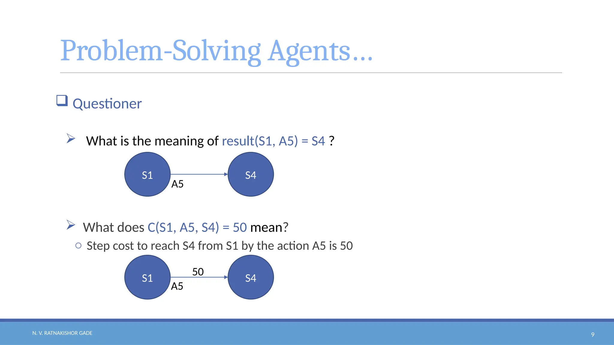
N. V. RATNAKISHORGADE 9
Problem-Solving Agents…
Questioner
What is the meaning of result(S1, A5) = S4 ?
What does C(S1, A5, S4) = 50 mean?
o Step cost to reach S4 from S1 by the action A5 is 50
S1 S4
A5
S1 S4
A5
50
10.
N. V. RATNAKISHORGADE 10
Example Problems
Toy Problems
8 – puzzle
8 – queens
Tic-Tac-Toe
. . .
Real – world Problems
Vacuum Cleaner
Airline Travel Problem
Travelling Salesman Problem
. . .
11.
N. V. RATNAKISHORGADE 11
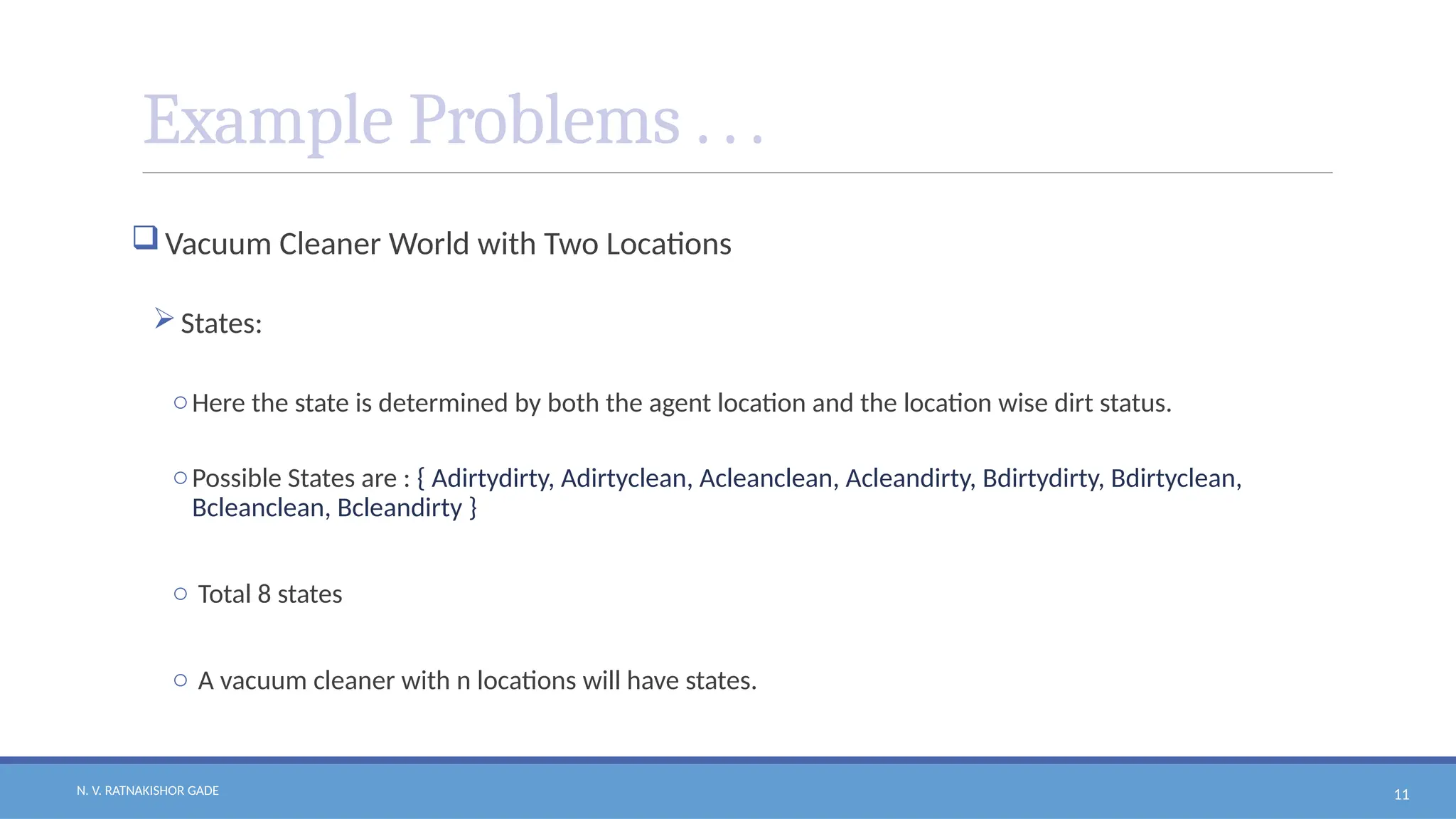
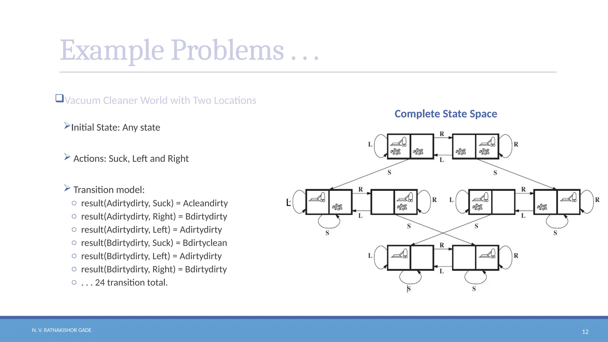
Example Problems . . .
Vacuum Cleaner World with Two Locations
States:
oHere the state is determined by both the agent location and the location wise dirt status.
oPossible States are : { Adirtydirty, Adirtyclean, Acleanclean, Acleandirty, Bdirtydirty, Bdirtyclean,
Bcleanclean, Bcleandirty }
o Total 8 states
o A vacuum cleaner with n locations will have states.
12.
N. V. RATNAKISHORGADE 12
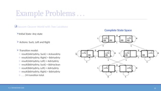
Example Problems . . .
Vacuum Cleaner World with Two Locations
Initial State: Any state
Actions: Suck, Left and Right
Transition model:
o result(Adirtydirty, Suck) = Acleandirty
o result(Adirtydirty, Right) = Bdirtydirty
o result(Adirtydirty, Left) = Adirtydirty
o result(Bdirtydirty, Suck) = Bdirtyclean
o result(Bdirtydirty, Left) = Adirtydirty
o result(Bdirtydirty, Right) = Bdirtydirty
o . . . 24 transition total.
Complete State Space
L
13.
N. V. RATNAKISHORGADE 13
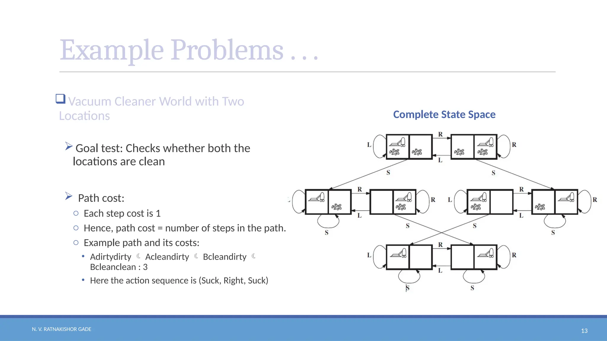
Example Problems . . .
Vacuum Cleaner World with Two
Locations
Goal test: Checks whether both the
locations are clean
Path cost:
o Each step cost is 1
o Hence, path cost = number of steps in the path.
o Example path and its costs:
• Adirtydirty Acleandirty Bcleandirty
Bcleanclean : 3
• Here the action sequence is (Suck, Right, Suck)
Complete State Space
14.
N. V. RATNAKISHORGADE 14
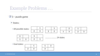
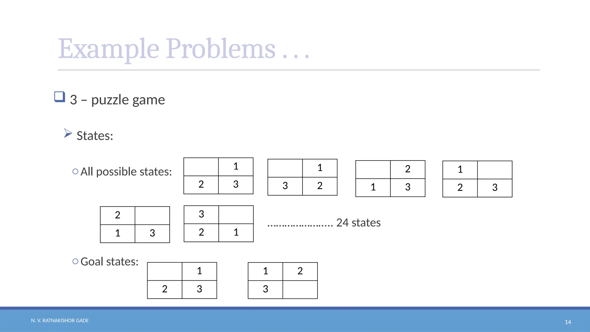
Example Problems . . .
3 – puzzle game
States:
oAll possible states:
………………….. 24 states
oGoal states:
2
1 3
1
2 3
2
1 3
1
3 2
1
2 3
3
2 1
1
2 3
1 2
3
15.
N. V. RATNAKISHORGADE 15
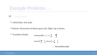
Example Problems . . .
3 – puzzle game
Initial State: Any state
Actions: Movement of blank space Left, Right, Up or Down.
Transition Model: 𝑟𝑒𝑠𝑢𝑙𝑡 ¿ ¿=
1 ∎
2 3
𝑟𝑒𝑠𝑢𝑙𝑡 (∎ 1
2 3
, Down)=
2 1
∎ 3
. . . 96 transitions total
16.
N. V. RATNAKISHORGADE 16
Example Problems . . .
3 – puzzle game
Goal test: Checks whether the state matches one of the goal configurations
mentioned above.
Path cost:
oEach step cost is 1
oSo the path cost is the number of steps in the path.
17.
N. V. RATNAKISHORGADE 17
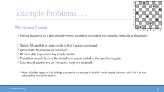
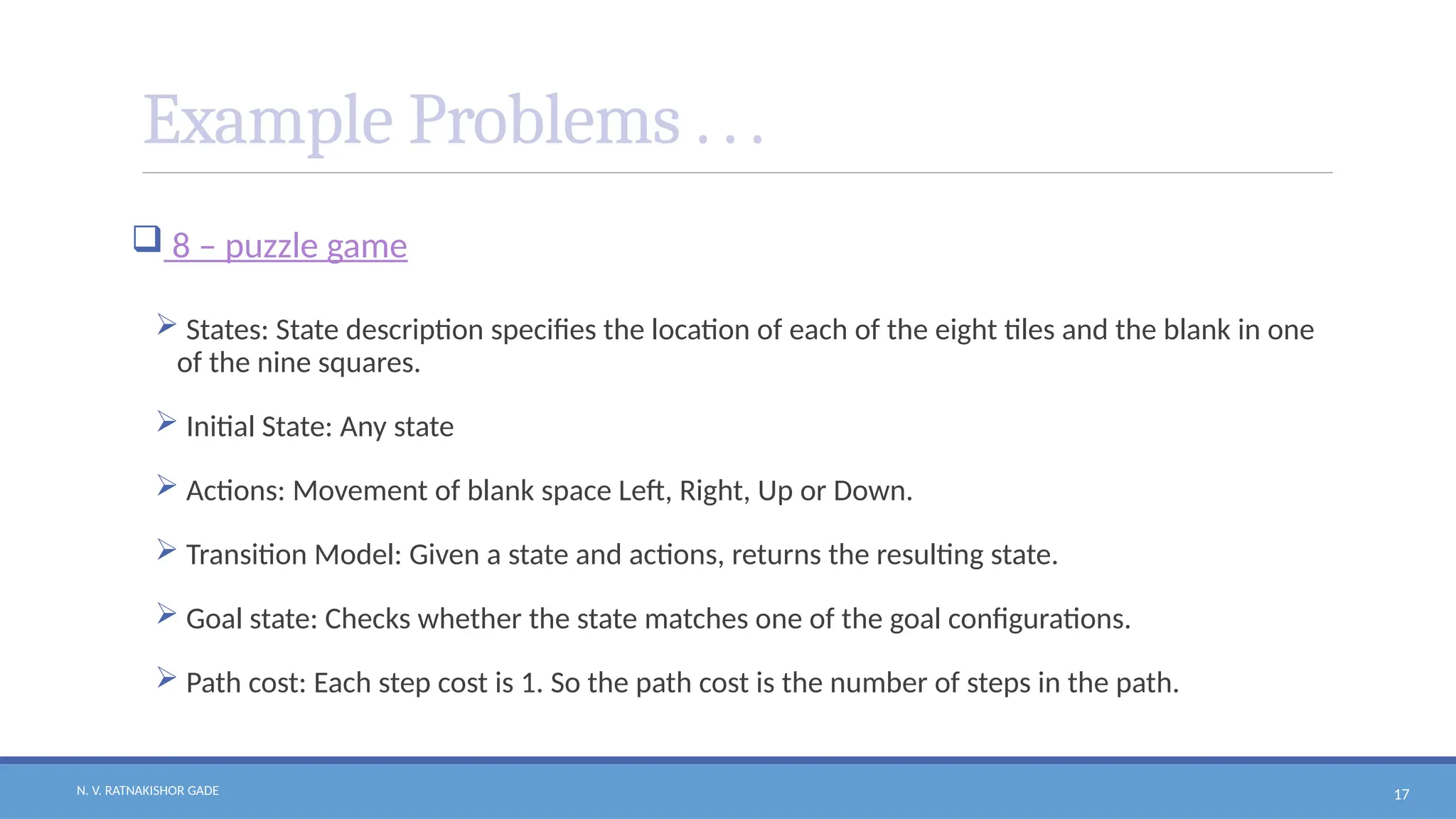
Example Problems . . .
8 – puzzle game
States: State description specifies the location of each of the eight tiles and the blank in one
of the nine squares.
Initial State: Any state
Actions: Movement of blank space Left, Right, Up or Down.
Transition Model: Given a state and actions, returns the resulting state.
Goal state: Checks whether the state matches one of the goal configurations.
Path cost: Each step cost is 1. So the path cost is the number of steps in the path.
18.
N. V. RATNAKISHORGADE 18
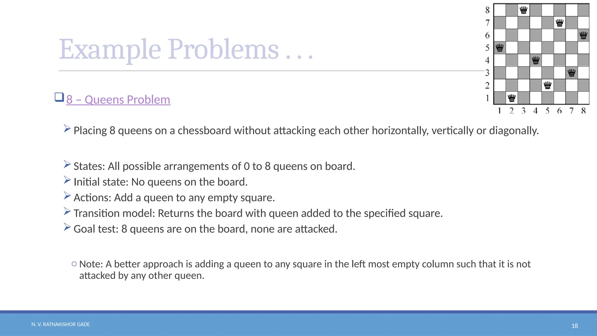
Example Problems . . .
8 – Queens Problem
Placing 8 queens on a chessboard without attacking each other horizontally, vertically or diagonally.
States: All possible arrangements of 0 to 8 queens on board.
Initial state: No queens on the board.
Actions: Add a queen to any empty square.
Transition model: Returns the board with queen added to the specified square.
Goal test: 8 queens are on the board, none are attacked.
o Note: A better approach is adding a queen to any square in the left most empty column such that it is not
attacked by any other queen.
19.
N. V. RATNAKISHORGADE 19
Example Problems . . .
Airline Travel Planner Problem – A route finding problem
States: Each state contains the location and other information such as current time, fare bases,
domestic/international etc.
Initial state: Specified by user.
Actions: Taking the flight from current location.
Transition model: State (Location) resulting from taking a flight.
Goal test: Checking that the user is at his destination.
Path cost: Depends on travel time, waiting time, distance, time of the day, type of plane, seat class,
immigration procedure and so on.
20.
N. V. RATNAKISHORGADE 20
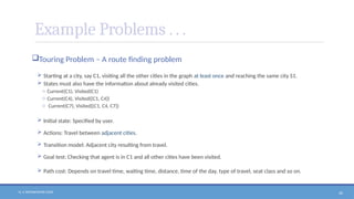
Example Problems . . .
Touring Problem – A route finding problem
Starting at a city, say C1, visiting all the other cities in the graph at least once and reaching the same city S1.
States must also have the information about already visited cities.
o Current(C1), Visited(C1)
o Current(C4), Visited({C1, C4})
o Current(C7), Visited({C1, C4, C7})
Initial state: Specified by user.
Actions: Travel between adjacent cities.
Transition model: Adjacent city resulting from travel.
Goal test: Checking that agent is in C1 and all other cities have been visited.
Path cost: Depends on travel time, waiting time, distance, time of the day, type of travel, seat class and so on.
21.
N. V. RATNAKISHORGADE 21
Example Problems . . .
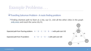
Travelling Salesman Problem– A route finding problem
Finding shortest path to Start at a city, say C1, visit all the other cities in the graph
only once and reach the same city S1.
Expected path from Touring problem:
Expected path from TS problem:
A B C D B A with path cost 110
A B C D A with path cost 120
22.
N. V. RATNAKISHORGADE 22
Example Problems . . .
A VLSI Layout Problem
Positioning millions of components and connections on a chip to minimize area,
minimize circuit delays, minimize power consumption and maximizing manufacturing
yield.
Robot Navigation
Generalization of route-finding problem
Robot can move in continuous space with infinite set of possible states and actions.
23.
N. V. RATNAKISHORGADE 23
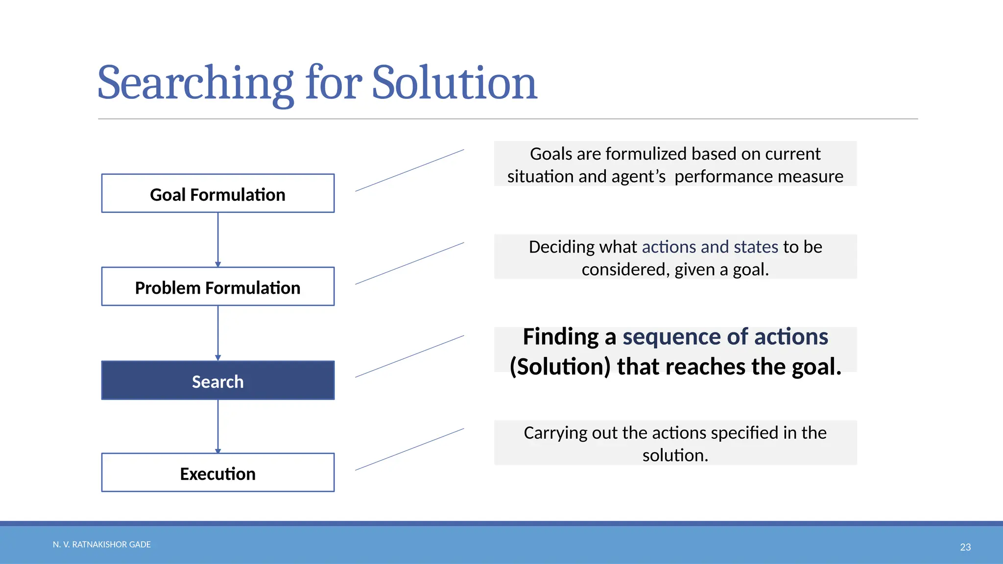
Searching for Solution
Goal Formulation
Problem Formulation
Search
Execution
Goals are formulized based on current
situation and agent’s performance measure
Deciding what actions and states to be
considered, given a goal.
Finding a sequence of actions
(Solution) that reaches the goal.
Carrying out the actions specified in the
solution.
24.
N. V. RATNAKISHORGADE 24
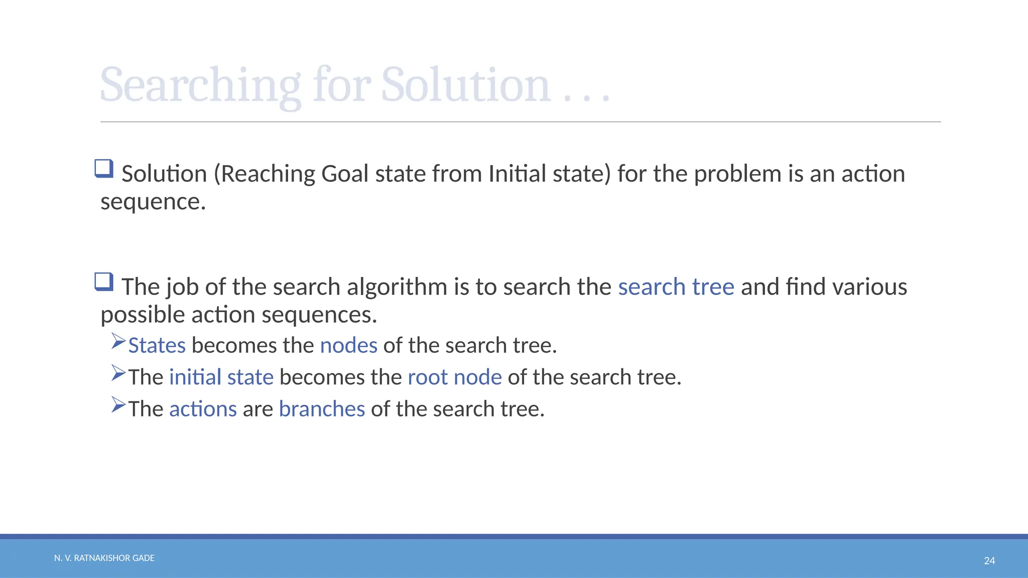
Searching for Solution . . .
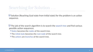
Solution (Reaching Goal state from Initial state) for the problem is an action
sequence.
The job of the search algorithm is to search the search tree and find various
possible action sequences.
States becomes the nodes of the search tree.
The initial state becomes the root node of the search tree.
The actions are branches of the search tree.
25.
N. V. RATNAKISHORGADE 25
Searching for Solution . . .
Some Key Terms
State Expansion: Generating a new set of states by applying each possible action to
the current state.
Frontier / Open list: Set of all the states available for expansion.
Explored list / Closed list: Set of all the expanded states.
Search Strategy: Decides which state to expand next.
26.
N. V. RATNAKISHORGADE 26
Searching for Solution . . .
ADD
Initial State
Frontier: [ADD]
Explored_list: []
ADD
After Expanding ADD
L
ACD BDD
S R
Frontier: [BDD, ACD]
Explored_list: [ADD]
ADD
After Expanding ACD
L
S/L
ACD BDD
S R
R
BCD
Frontier: [BDD, BCD]
Explored_list: [ADD, ACD]
27.
N. V. RATNAKISHORGADE 27
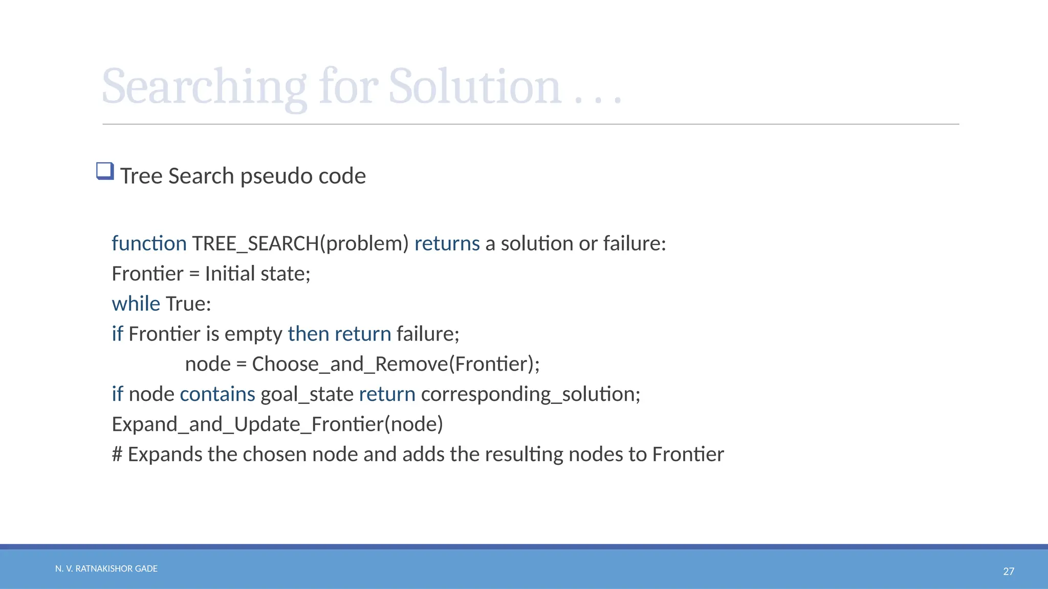
Searching for Solution . . .
Tree Search pseudo code
function TREE_SEARCH(problem) returns a solution or failure:
Frontier = Initial state;
while True:
if Frontier is empty then return failure;
node = Choose_and_Remove(Frontier);
if node contains goal_state return corresponding_solution;
Expand_and_Update_Frontier(node)
# Expands the chosen node and adds the resulting nodes to Frontier
28.
N. V. RATNAKISHORGADE 28
Searching for Solution . . .
Graph Search pseudo code – Handles the repeated states with the help of explored list.
function GRAPH_SEARCH(problem) returns a solution or failure:
Frontier = Initial state;
Explored_list = []
while True:
if Frontier is empty then return failure;
node = Choose_and_Remove(Frontier);
if node contains goal_state return corresponding_solution;
Explored_list.append(node)
Expand_and_Update_Frontier_(node)
# Expands the chosen node and adds the resulting nodes to Frontier
only if not in the Frontier or Explored_list.
29.
N. V. RATNAKISHORGADE 29
Searching for Solution . . .
Mention the contents of Frontier and Explored_list of the following.
Frontier: [4]
Explored_list: [0, 1, 2, 3]
Frontier: [Arad]
Explored_list: []
Frontier: [Sibiu, Timisoara, Zerind ]
Explored_list: [Arad]
Frontier:
Explored_list: [Arad, Sibiu]
[Timisoara, Zerind, Fagaras, Oradea, R V ]
30.
N. V. RATNAKISHORGADE 30
Searching for Solution . . .
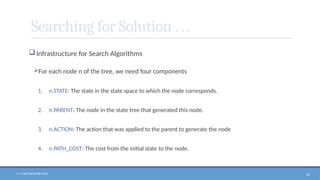
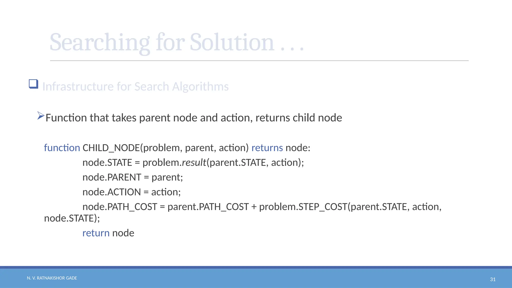
Infrastructure for Search Algorithms
For each node n of the tree, we need four components
1. n.STATE: The state in the state space to which the node corresponds.
2. n.PARENT: The node in the state tree that generated this node.
3. n.ACTION: The action that was applied to the parent to generate the node
4. n.PATH_COST: The cost from the initial state to the node.
31.
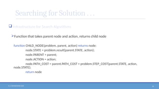
N. V. RATNAKISHORGADE 31
Searching for Solution . . .
Infrastructure for Search Algorithms
Function that takes parent node and action, returns child node
function CHILD_NODE(problem, parent, action) returns node:
node.STATE = problem.result(parent.STATE, action);
node.PARENT = parent;
node.ACTION = action;
node.PATH_COST = parent.PATH_COST + problem.STEP_COST(parent.STATE, action,
node.STATE);
return node
32.
N. V. RATNAKISHORGADE 32
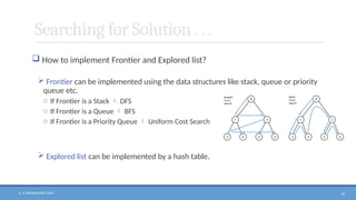
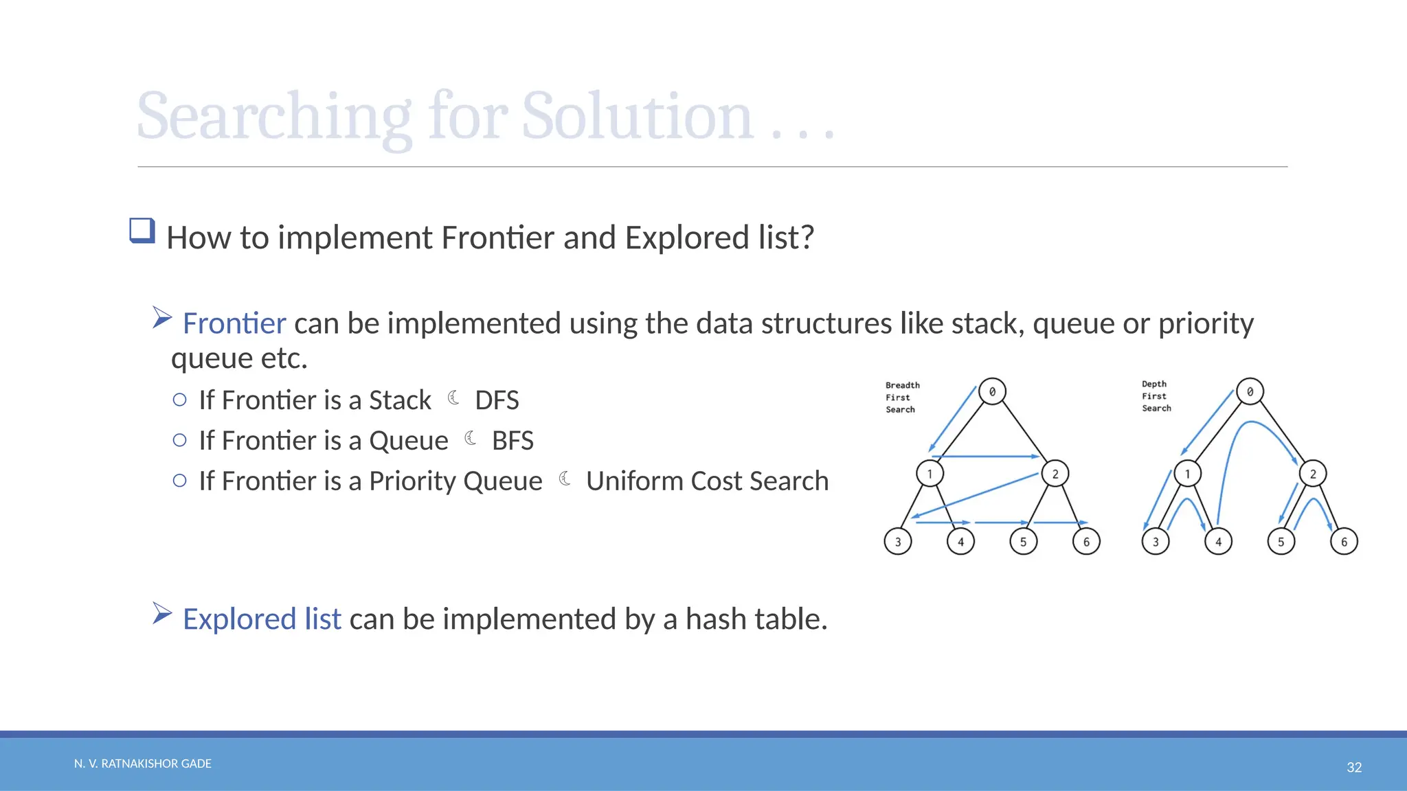
Searching for Solution . . .
How to implement Frontier and Explored list?
Frontier can be implemented using the data structures like stack, queue or priority
queue etc.
o If Frontier is a Stack DFS
o If Frontier is a Queue BFS
o If Frontier is a Priority Queue Uniform Cost Search
Explored list can be implemented by a hash table.
33.
N. V. RATNAKISHORGADE 33
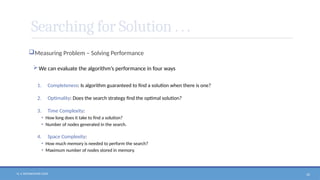
Searching for Solution . . .
Measuring Problem – Solving Performance
We can evaluate the algorithm’s performance in four ways
1. Completeness: Is algorithm guaranteed to find a solution when there is one?
2. Optimality: Does the search strategy find the optimal solution?
3. Time Complexity:
• How long does it take to find a solution?
• Number of nodes generated in the search.
4. Space Complexity:
• How much memory is needed to perform the search?
• Maximum number of nodes stored in memory.
34.
N. V. RATNAKISHORGADE 34
Searching for Solution . . .
Measuring Problem – Solving Performance
Three quantities used to express complexity
o b:
• Branching factor
• Maximum number of successors of any node
o d:
• Depth of the shallowest goal
• The number of steps along the path from the route
o m:
• Maximum length of any path in the state space
35.
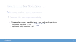
N. V. RATNAKISHORGADE 35
Searching for Solution . . .
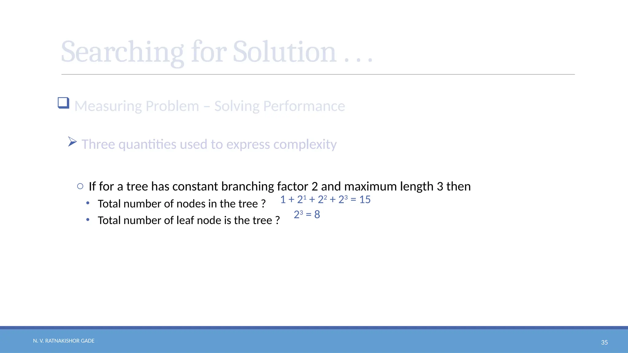
Measuring Problem – Solving Performance
Three quantities used to express complexity
o If for a tree has constant branching factor 2 and maximum length 3 then
• Total number of nodes in the tree ?
• Total number of leaf node is the tree ?
1 + 21
+ 22
+ 23
= 15
23
= 8
36.
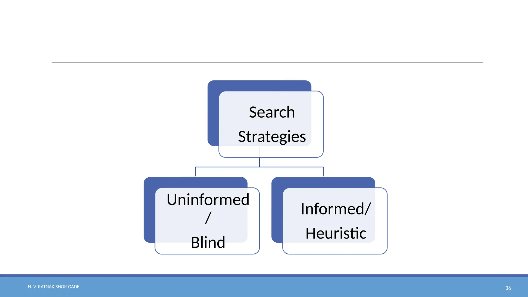
N. V. RATNAKISHORGADE 36
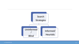
Search
Strategies
Uninformed
/
Blind
Informed/
Heuristic
37.
N. V. RATNAKISHORGADE 37
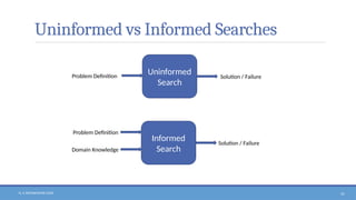
Uninformed vs Informed Searches
Informed
Search
Problem Definition
Domain Knowledge
Solution / Failure
Uninformed
Search
Problem Definition Solution / Failure
38.
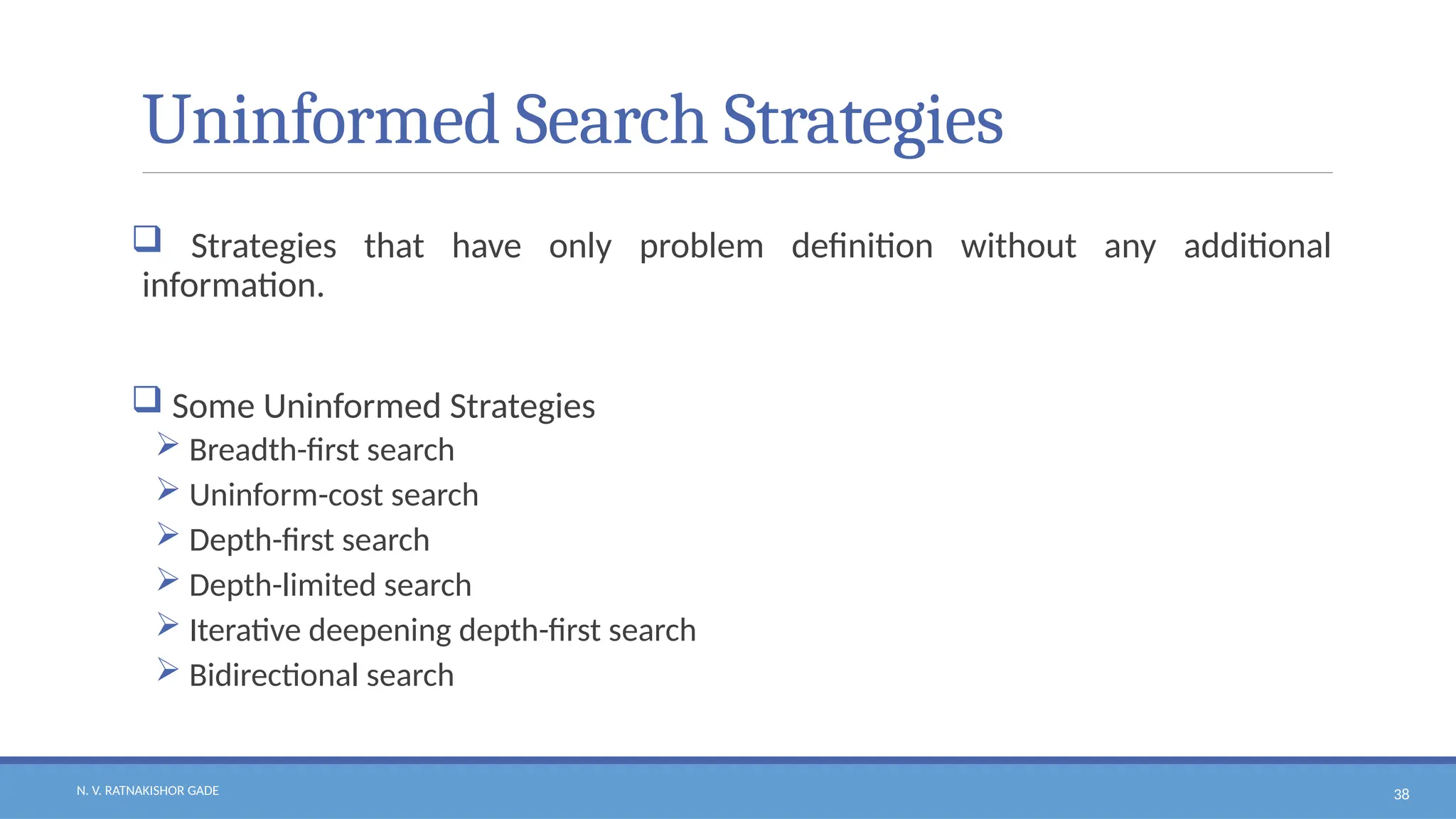
N. V. RATNAKISHORGADE 38
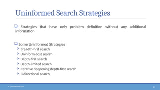
Uninformed Search Strategies
Strategies that have only problem definition without any additional
information.
Some Uninformed Strategies
Breadth-first search
Uninform-cost search
Depth-first search
Depth-limited search
Iterative deepening depth-first search
Bidirectional search
39.
N. V. RATNAKISHORGADE 39
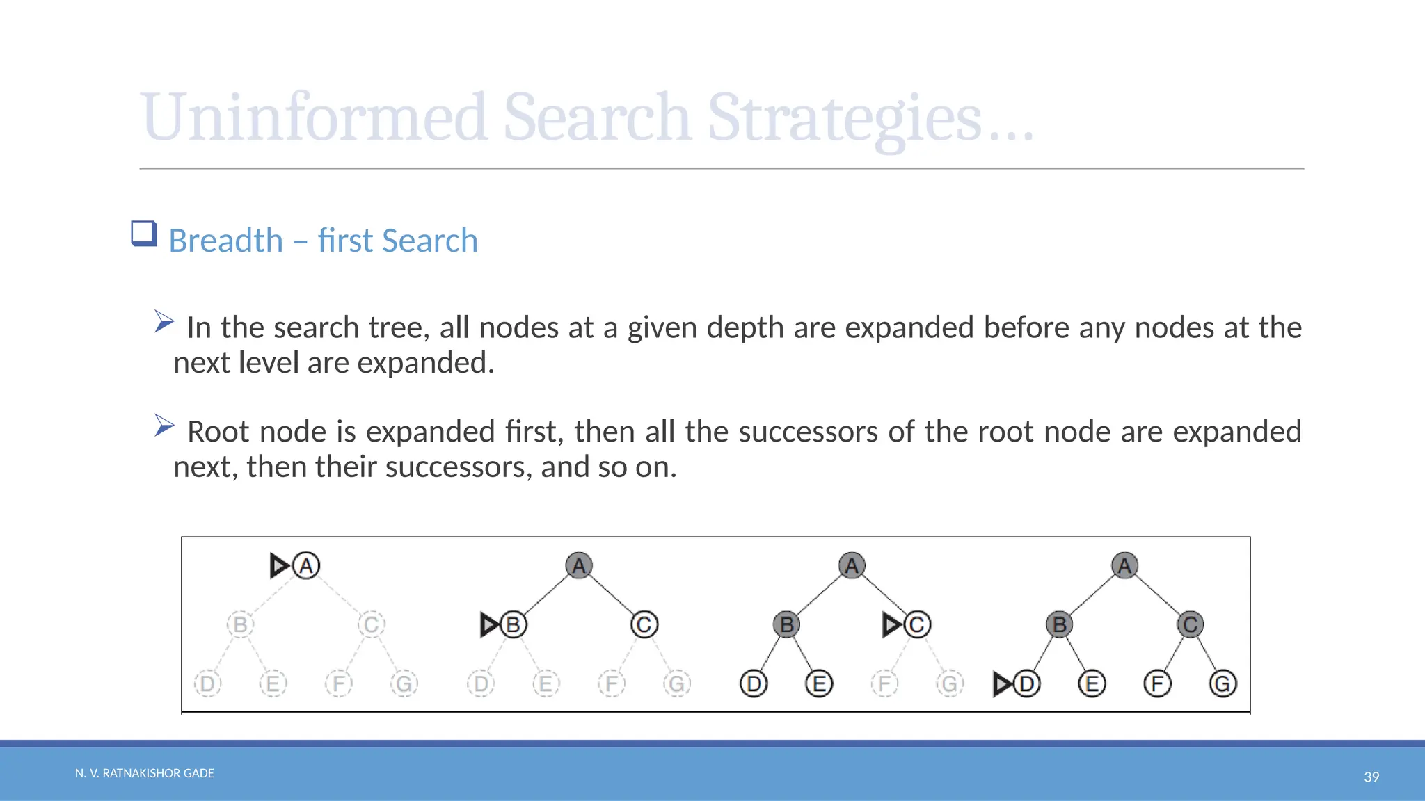
Uninformed Search Strategies…
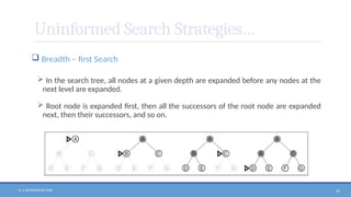
Breadth – first Search
In the search tree, all nodes at a given depth are expanded before any nodes at the
next level are expanded.
Root node is expanded first, then all the successors of the root node are expanded
next, then their successors, and so on.
40.
N. V. RATNAKISHORGADE 40
Uninformed Search Strategies…
Breadth – first Search
BFS can be implemented by using a FIFO Queue for the Frontier.
Function Pseudo code
function BFS(problem) returns a solution or failure:
Frontier Create a Queue and insert a node with initial state;
Explored_list = []
while True:
if Frontier is empty then return failure;
node = Frontier.deQueue(); # Removes the first inserted node
Explored_list.append(node);
successor_nodes = Expand(nodes);
for each node in successor_nodes:
if node contains goal_state return corresponding_solution;
if node not in (Frontier or Explored_list) then
Frontier.enQueue(node)
41.
N. V. RATNAKISHORGADE 41
Uninformed Search Strategies…
Breadth – first Search
function BREADTH_FIRST_SEARCH(problem) returns solution or failure:
node.STATE = problem.INITIAL_STATE;
node.PATH_COST = 0;
if problem.GOAL_TEST(node) then return SOLUTION(node);
Frontier.enQueue(node);
Explored_list = [];
while True:
if Frontier is empty then return failure;
node = Frontier.deQueue();
Explored_list.append(node.STATE);
for each action in problem.ACTIONS(node.STATE) do:
child = CHILD_NODE(problem, node, action);
if child.STATE not in (Frontier or Explored_list) then
if problem.GOAL_TEST(child.STATE) then return SOLUTION(child)
Frontier.enQueue(child)
42.
N. V. RATNAKISHORGADE 42
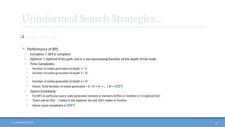
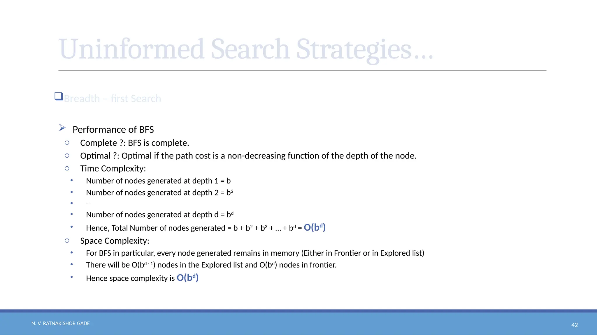
Uninformed Search Strategies…
Breadth – first Search
Performance of BFS
o Complete ?: BFS is complete.
o Optimal ?: Optimal if the path cost is a non-decreasing function of the depth of the node.
o Time Complexity:
• Number of nodes generated at depth 1 = b
• Number of nodes generated at depth 2 = b2
• ….
• Number of nodes generated at depth d = bd
• Hence, Total Number of nodes generated = b + b2
+ b3
+ … + bd
= O(bd
)
o Space Complexity:
• For BFS in particular, every node generated remains in memory (Either in Frontier or in Explored list)
• There will be O(bd - 1
) nodes in the Explored list and O(bd
) nodes in frontier.
• Hence space complexity is O(bd
)
43.
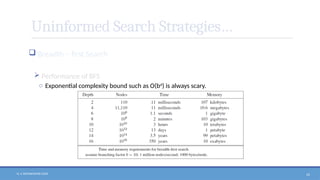
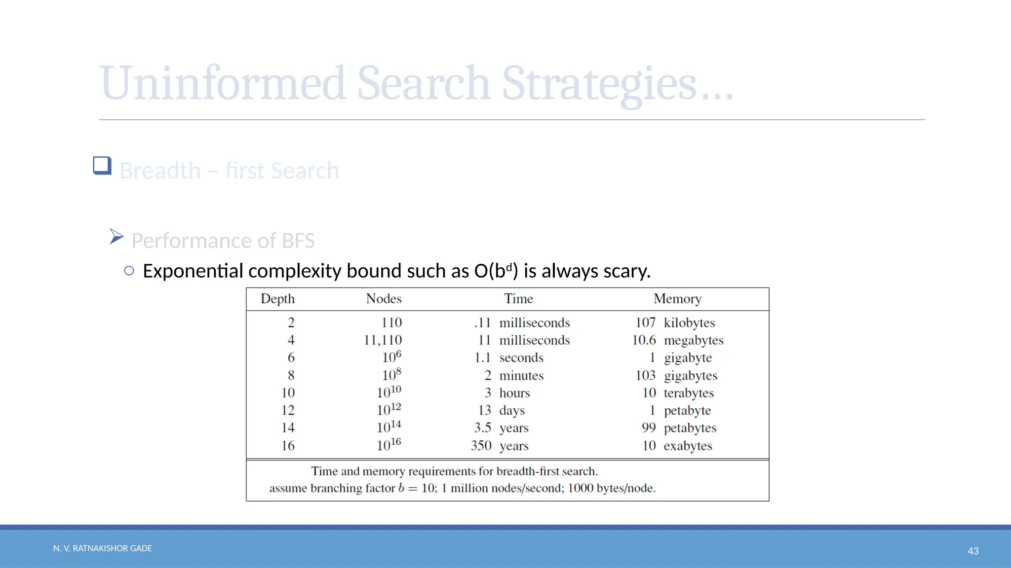
N. V. RATNAKISHORGADE 43
Uninformed Search Strategies…
Breadth – first Search
Performance of BFS
o Exponential complexity bound such as O(bd
) is always scary.
44.
N. V. RATNAKISHORGADE 44
Uninformed Search Strategies…
Uniform - Cost Search
When all step costs are equal only, BFS is optimal.
Uniform-cost search is a simple extension of BSF, which is optimal for any step cost.
Instead of expanding shallowest node, UCS expands the node n with the lowest path
cost g(n).
This is done by using a priority queue ordered by path cost, g(n) as Frontier.
In UCS, the complexities are characterized by costs but not easily by b and d.
45.
N. V. RATNAKISHORGADE 45
Uninformed Search Strategies…
Uniform - Cost Search
PQ EL
A []
PQ EL
C(9) B(5) [A]
PQ EL
E(13) D(7) C(9) [A, B]
PQ EL
G(13) E(13) C(9) [A, B, D]
46.
N. V. RATNAKISHORGADE 46
Uninformed Search Strategies…
Uniform - Cost Search
Function Pseudo code
function UCS(problem) returns a solution or failure:
Frontier Create a path cost based Priority Queue and insert a node with initial state;
Explored_list = []
while True:
if Frontier is empty then return failure;
node = Frontier.deQueue(); # Chooses a node with lowest path
cost
Explored_list.append(node);
successor_nodes = Expand(nodes);
for each node in successor_nodes :
if node contains goal_state return corresponding_solution;
if node not in (Frontier or Explored_list) then
Frontier.enQueue(node)
if node is in Frontier with more path_cost replace Frontier node.
47.
N. V. RATNAKISHORGADE 47
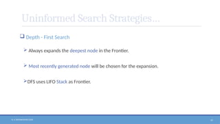
Uninformed Search Strategies…
Depth - First Search
Always expands the deepest node in the Frontier.
Most recently generated node will be chosen for the expansion.
DFS uses LIFO Stack as Frontier.
48.
N. V. RATNAKISHORGADE 48
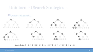
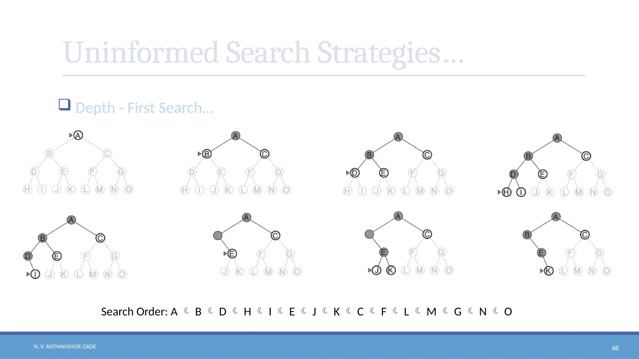
Uninformed Search Strategies…
Depth - First Search…
Search Order: A B D H I E J K C F L M G N O
49.
N. V. RATNAKISHORGADE 49
Uninformed Search Strategies…
Depth - First Search…
Function Pseudo code
function DFS(problem) returns a solution or failure:
Frontier Create a stack and insert a node with initial state;
Explored_list = []
while True:
if Frontier is empty then return failure;
node = Frontier.Pop(); # Chooses a note that is inserted last.
Explored_list.append(node);
successor_nodes = Expand(nodes);
for each node in successor_nodes :
if node contains goal_state return corresponding_solution;
if node not in (Frontier or Explored_list) then Frontier.Push(node)
50.
N. V. RATNAKISHORGADE 50
Uninformed Search Strategies…
Depth – First Search…
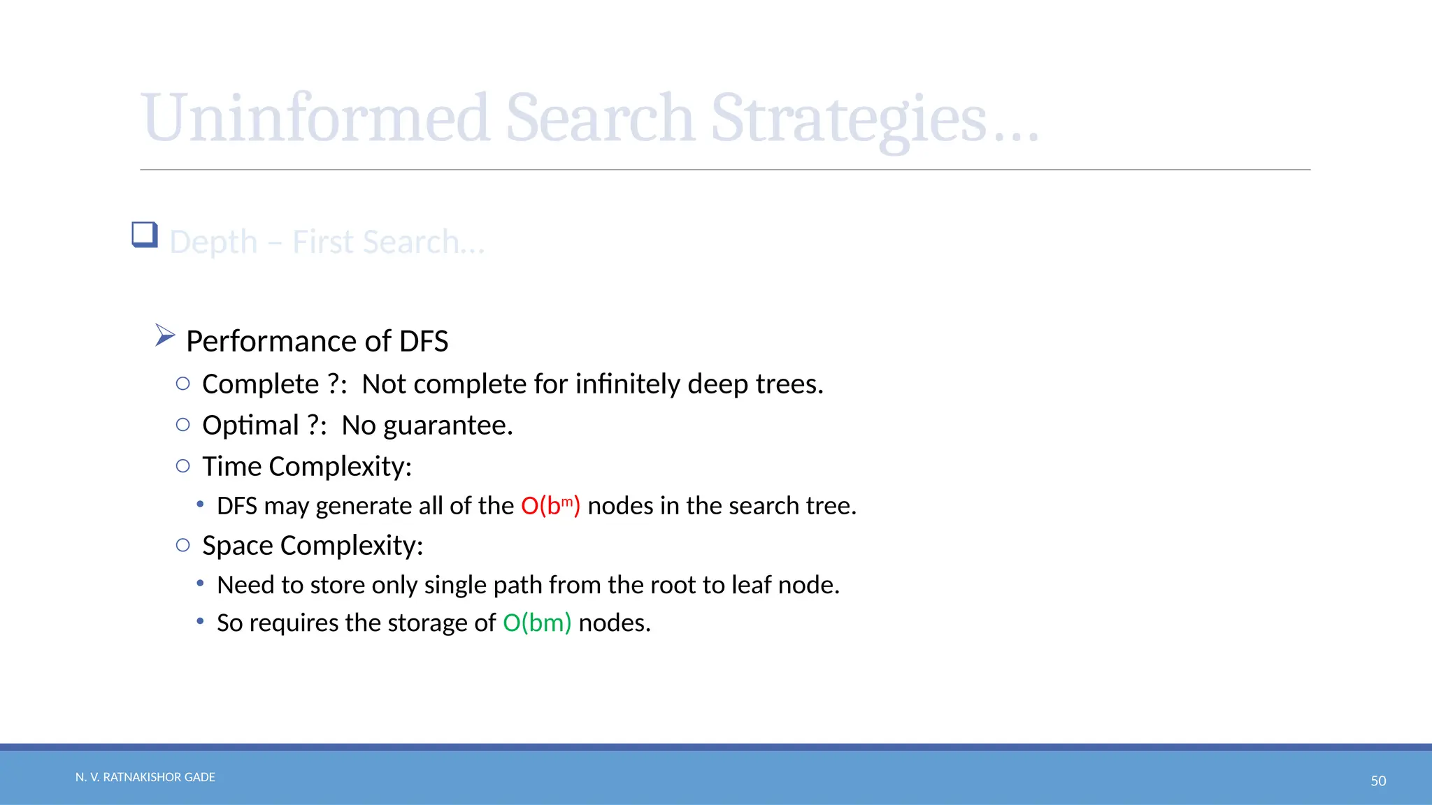
Performance of DFS
o Complete ?: Not complete for infinitely deep trees.
o Optimal ?: No guarantee.
o Time Complexity:
• DFS may generate all of the O(bm
) nodes in the search tree.
o Space Complexity:
• Need to store only single path from the root to leaf node.
• So requires the storage of O(bm) nodes.
51.
N. V. RATNAKISHORGADE 51
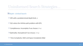
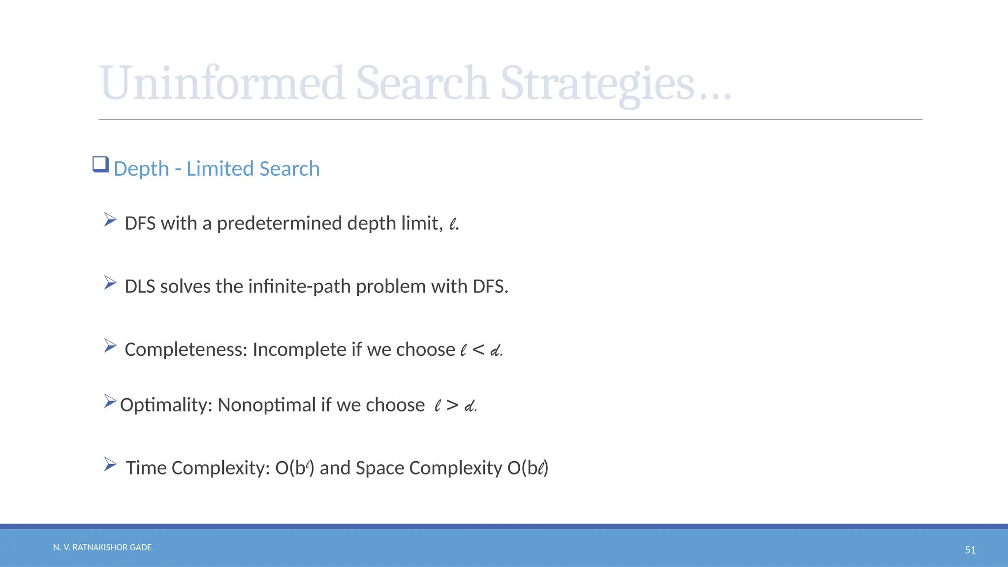
Uninformed Search Strategies…
Depth - Limited Search
DFS with a predetermined depth limit, l.
DLS solves the infinite-path problem with DFS.
Completeness: Incomplete if we choose l < d.
Optimality: Nonoptimal if we choose l > d.
Time Complexity: O(bl
) and Space Complexity O(bl)
52.
N. V. RATNAKISHORGADE 52
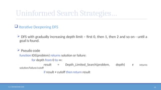
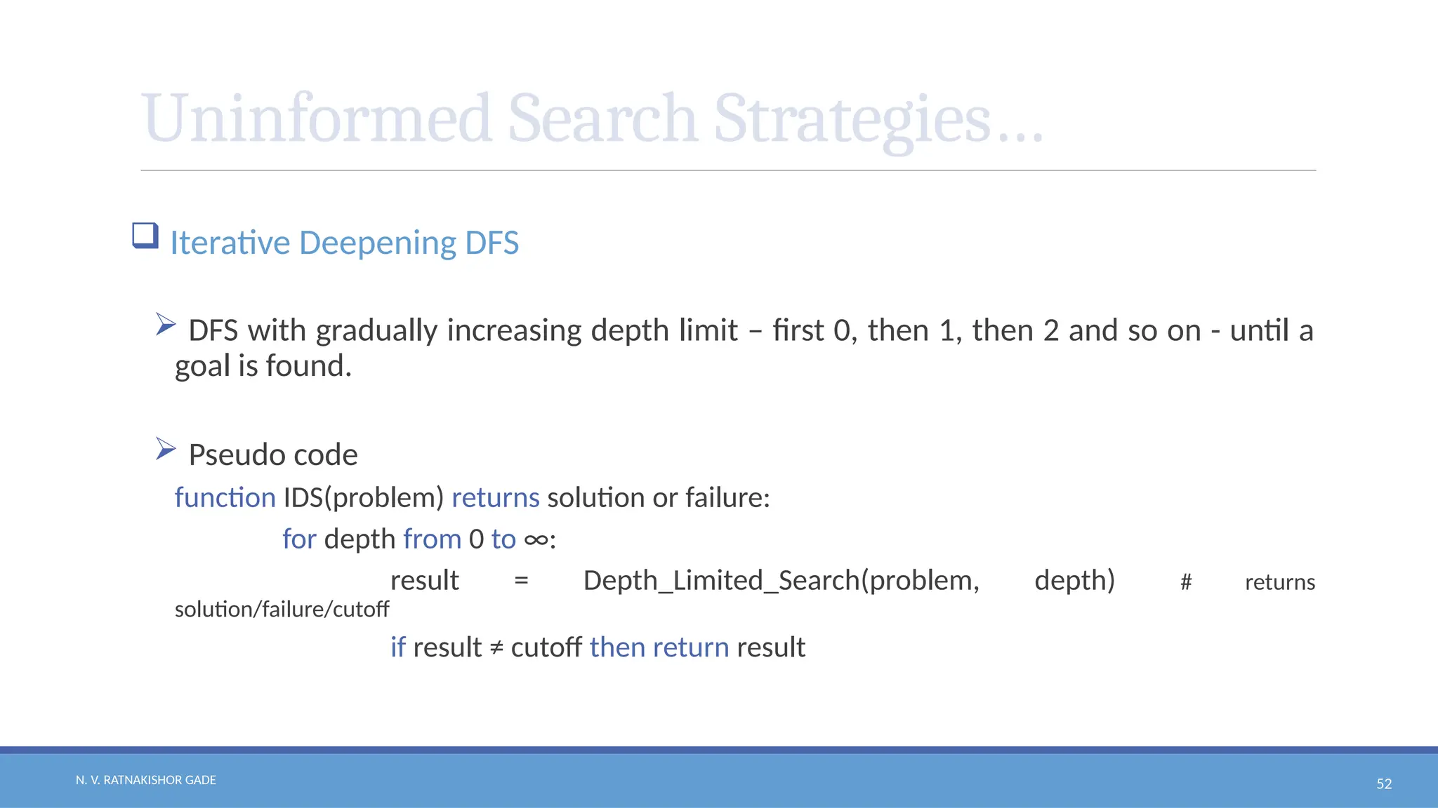
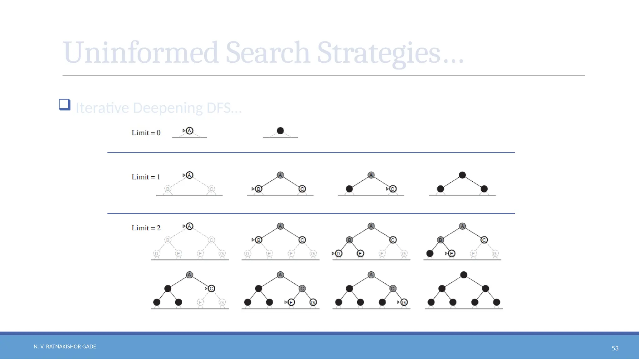
Uninformed Search Strategies…
Iterative Deepening DFS
DFS with gradually increasing depth limit – first 0, then 1, then 2 and so on - until a
goal is found.
Pseudo code
function IDS(problem) returns solution or failure:
for depth from 0 to ∞:
result = Depth_Limited_Search(problem, depth) # returns
solution/failure/cutoff
if result ≠ cutoff then return result
53.
N. V. RATNAKISHORGADE 53
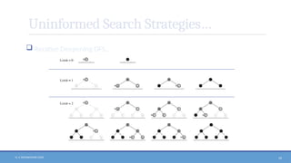
Uninformed Search Strategies…
Iterative Deepening DFS…
54.
N. V. RATNAKISHORGADE 54
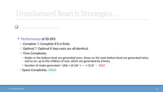
Uninformed Search Strategies…
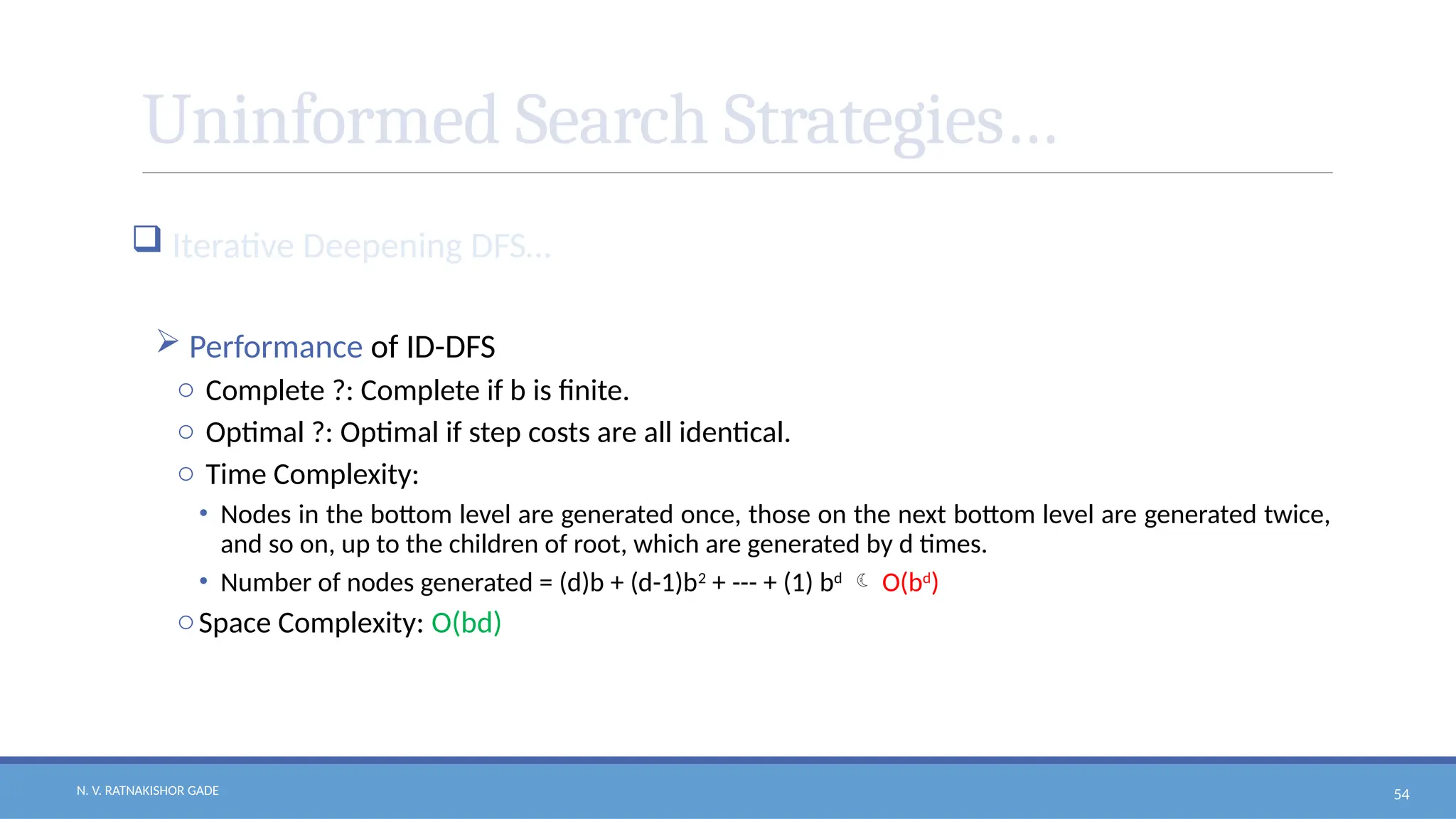
Iterative Deepening DFS…
Performance of ID-DFS
o Complete ?: Complete if b is finite.
o Optimal ?: Optimal if step costs are all identical.
o Time Complexity:
• Nodes in the bottom level are generated once, those on the next bottom level are generated twice,
and so on, up to the children of root, which are generated by d times.
• Number of nodes generated = (d)b + (d-1)b2
+ --- + (1) bd
O(bd
)
oSpace Complexity: O(bd)
55.
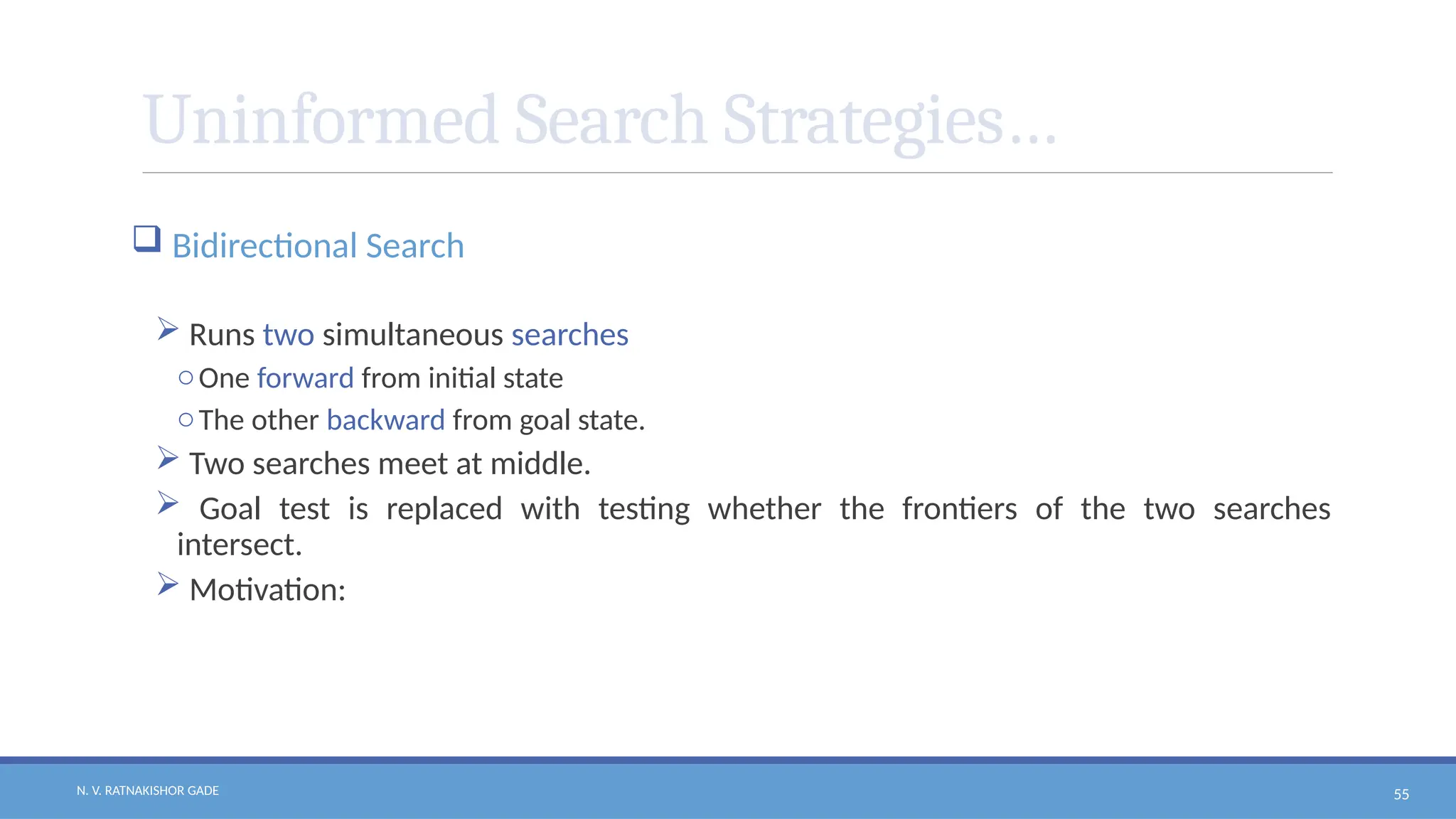
N. V. RATNAKISHORGADE 55
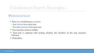
Uninformed Search Strategies…
Bidirectional Search
Runs two simultaneous searches
oOne forward from initial state
oThe other backward from goal state.
Two searches meet at middle.
Goal test is replaced with testing whether the frontiers of the two searches
intersect.
Motivation:
56.
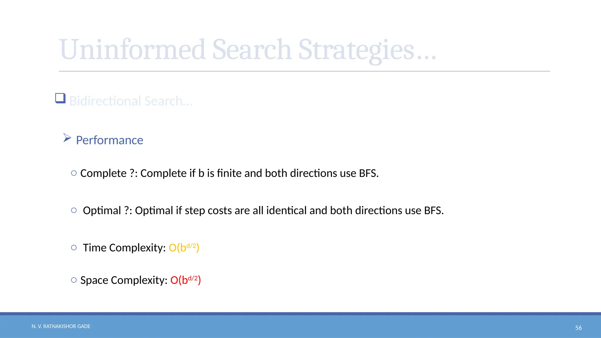
N. V. RATNAKISHORGADE 56
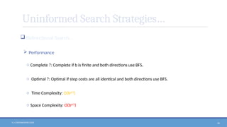
Uninformed Search Strategies…
Bidirectional Search…
Performance
o Complete ?: Complete if b is finite and both directions use BFS.
o Optimal ?: Optimal if step costs are all identical and both directions use BFS.
o Time Complexity: O(bd/2
)
o Space Complexity: O(bd/2
)
57.
N. V. RATNAKISHORGADE 57
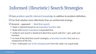
Informed (Heuristic) Search Strategies
Uses problem-specific (domain) knowledge in addition to problem definition.
Can find solution more effectively than an uninformed strategy.
General – approach Best-first search.
Node is selected based on an Evaluation function, f(n).
Node with lowest evaluation is expanded first.
Uniform cost search is identical to Best-first search with f(n) = g(n), path cost
function.
In most of the Best-first search strategies, a Heuristic function h(n) acts as a
component of the f(n).
h(n) = Estimated cost of the cheapest path from the node n to a goal node.
58.
N. V. RATNAKISHORGADE 58
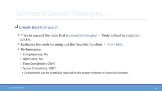
Informed Search Strategies…
Greedy Best-first Search
Tries to expand the node that is closest to the goal likely to lead to a solution
quickly.
Evaluates the node by using just the heuristic function f(n) = h(n).
Performance:
o Completeness: No
o Optimality: No
o Time Complexity: O(bm
)
o Space Complexity: O(bm
)
• Complexities can be drastically reduced by the proper selection of heuristic function.
59.
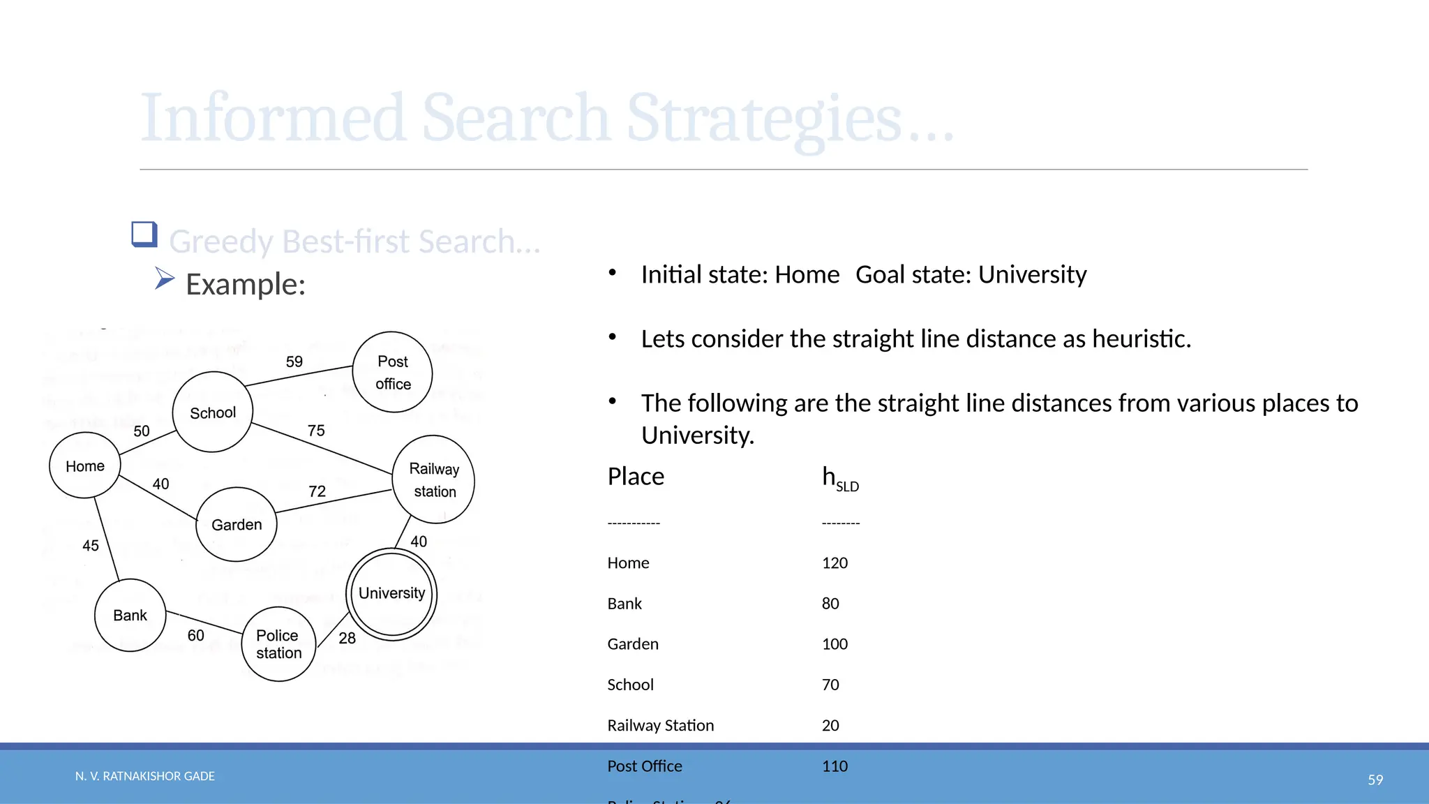
N. V. RATNAKISHORGADE 59
Informed Search Strategies…
Greedy Best-first Search…
Example: • Initial state: Home Goal state: University
• Lets consider the straight line distance as heuristic.
• The following are the straight line distances from various places to
University.
Place hSLD
----------- --------
Home 120
Bank 80
Garden 100
School 70
Railway Station 20
Post Office 110
60.
N. V. RATNAKISHORGADE 60
Informed Search Strategies…
Greedy Best-first Search…
Example:
PQ EL
H120 []
PQ EL
B80 G100 S70 [H]
PQ EL
B80 G100 R20 P110 [H, S]
PQ EL
B80 G100 P110 U0 [H, S, R]
Solution: Home School Railway station University
61.
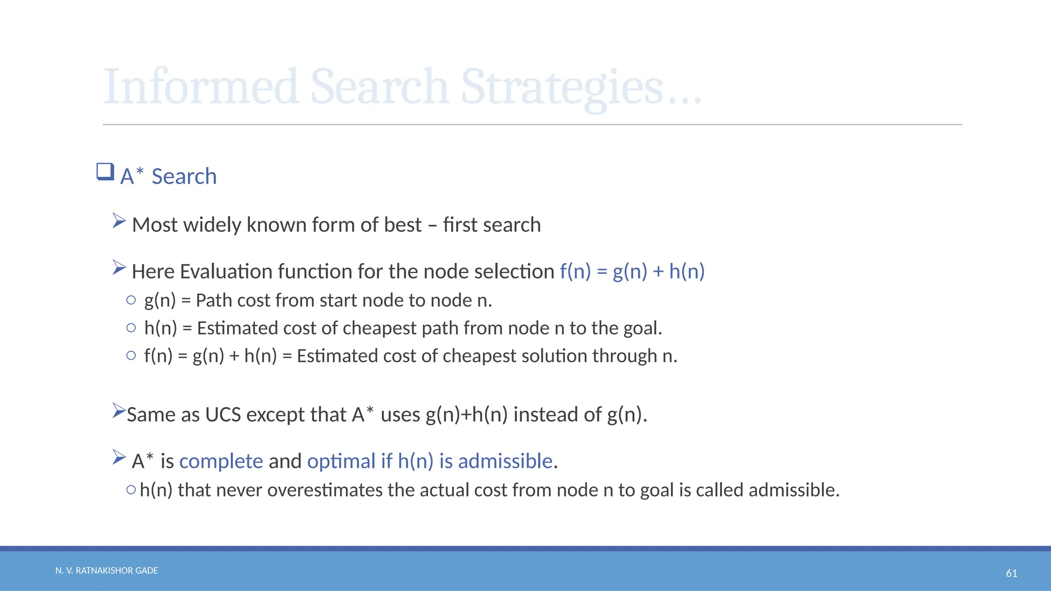
N. V. RATNAKISHORGADE 61
Informed Search Strategies…
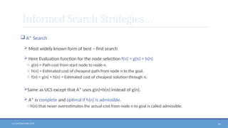
A* Search
Most widely known form of best – first search
Here Evaluation function for the node selection f(n) = g(n) + h(n)
o g(n) = Path cost from start node to node n.
o h(n) = Estimated cost of cheapest path from node n to the goal.
o f(n) = g(n) + h(n) = Estimated cost of cheapest solution through n.
Same as UCS except that A* uses g(n)+h(n) instead of g(n).
A* is complete and optimal if h(n) is admissible.
oh(n) that never overestimates the actual cost from node n to goal is called admissible.
62.
N. V. RATNAKISHORGADE 62
Informed Search Strategies…
A* Search…
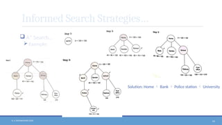
Example: • Initial state: Home Goal state: University
• Lets consider the straight line distance as heuristic.
• The following are the straight line distances from various places to
University.
Place hSLD
----------- --------
Home 120
Bank 80
Garden 100
School 70
Railway Station 20
Post Office 110
63.
N. V. RATNAKISHORGADE 63
Informed Search Strategies…
A* Search…
Example:
Solution: Home Bank Police station University
64.
N. V. RATNAKISHORGADE 64
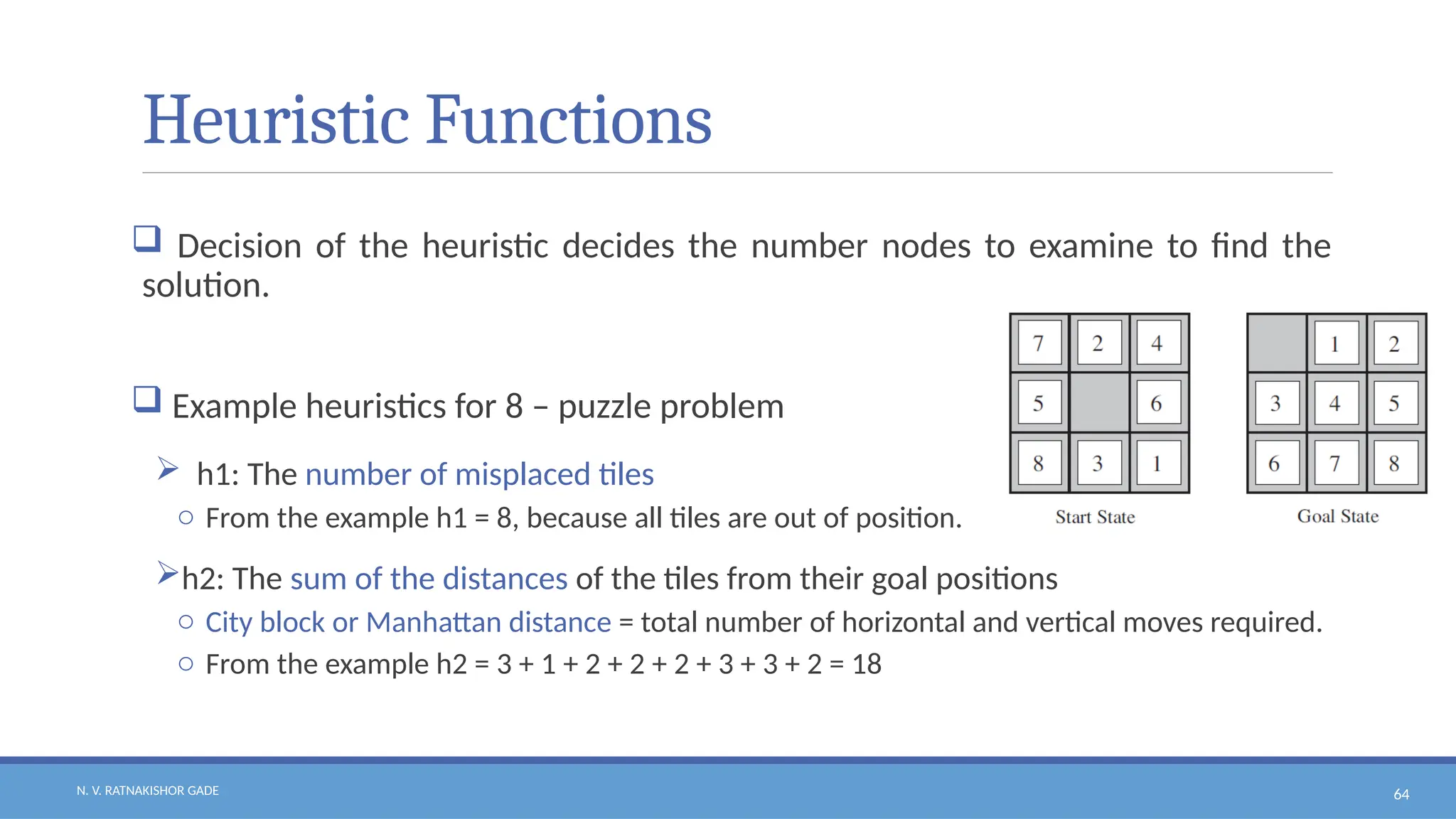
Heuristic Functions
Decision of the heuristic decides the number nodes to examine to find the
solution.
Example heuristics for 8 – puzzle problem
h1: The number of misplaced tiles
o From the example h1 = 8, because all tiles are out of position.
h2: The sum of the distances of the tiles from their goal positions
o City block or Manhattan distance = total number of horizontal and vertical moves required.
o From the example h2 = 3 + 1 + 2 + 2 + 2 + 3 + 3 + 2 = 18
65.
N. V. RATNAKISHORGADE 65
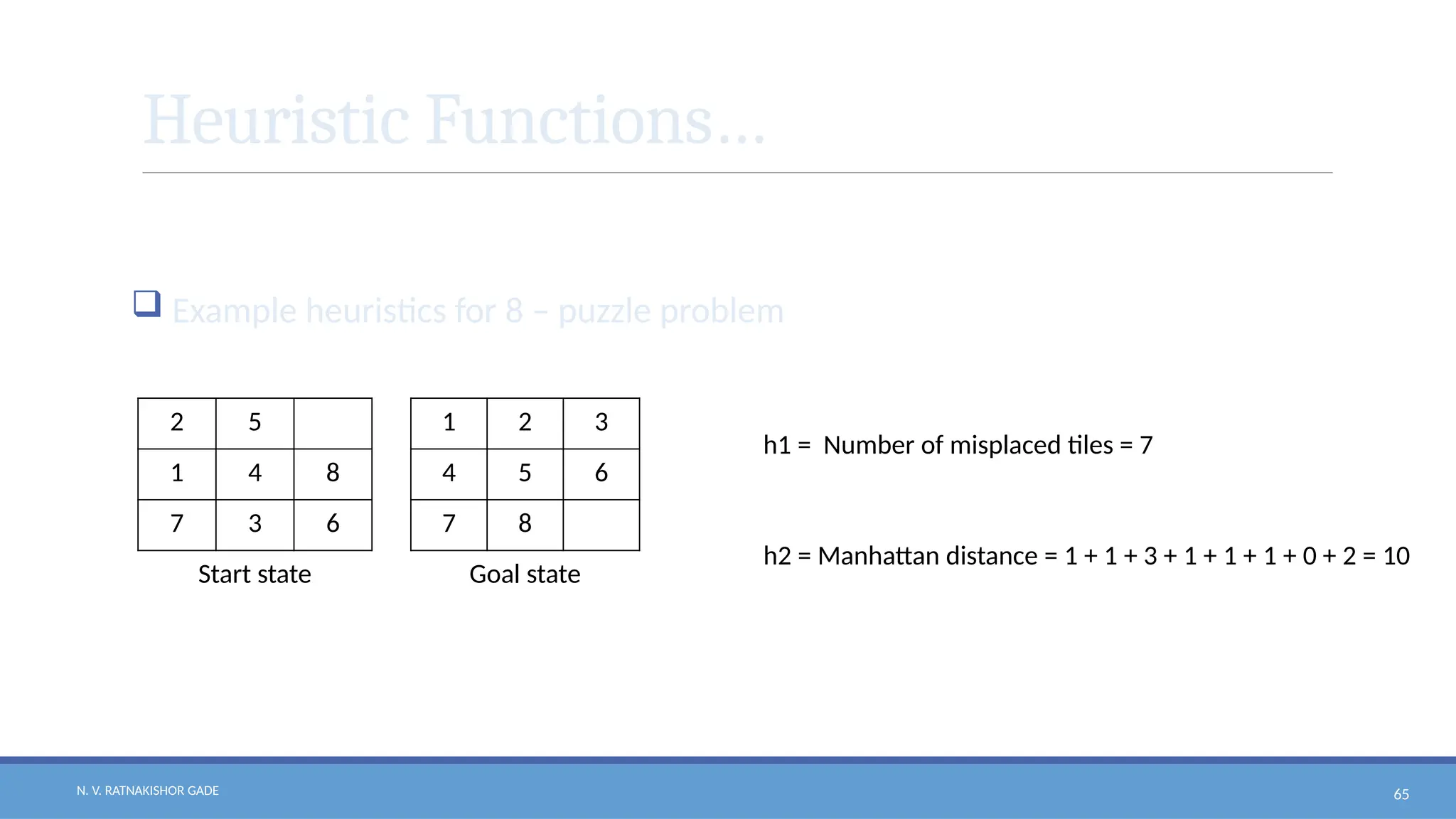
Heuristic Functions…
Example heuristics for 8 – puzzle problem
2 5
1 4 8
7 3 6
Start state
1 2 3
4 5 6
7 8
Goal state
h1 = Number of misplaced tiles = 7
h2 = Manhattan distance = 1 + 1 + 3 + 1 + 1 + 1 + 0 + 2 = 10
66.
N. V. RATNAKISHORGADE 66
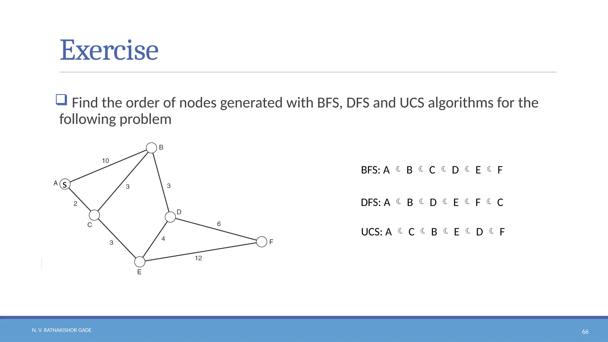
Exercise
Find the order of nodes generated with BFS, DFS and UCS algorithms for the
following problem
s
BFS: A B C D E F
DFS: A B D E F C
UCS: A C B E D F


![N. V. RATNAKISHOR GADE 4
Problem-Solving Agents…
Pseudo code for Simple Problem – Solving Agent:
action_sequence = [] # Action Sequence, initially empty
goal = null # Goal, initially Null
function Simple_Problem_Solving_Agent(percept) returns action:
state = UPDATE_STATE(state, percept) # State Update
if action_sequence is empty then:
goal = FORMULATE_GOAL(state) # Goal Formulation
problem = FORMULATE_PROBLEM(state, goal) # Problem Formulation
action_sequence = SEARCH(problem) # Searching to find the solution
action = FIRST(action_sequence) # Discharge action for execution
action_sequence = REST(action_sequence) # Remove the discharged action from action sequence
return action](https://image.slidesharecdn.com/ai-unit2-250906081612-e9583315/85/AI-Unit2_Artificial-intelligence-understanding-pptx-4-320.jpg)


![N. V. RATNAKISHOR GADE 26
Searching for Solution . . .
ADD
Initial State
Frontier: [ADD]
Explored_list: []
ADD
After Expanding ADD
L
ACD BDD
S R
Frontier: [BDD, ACD]
Explored_list: [ADD]
ADD
After Expanding ACD
L
S/L
ACD BDD
S R
R
BCD
Frontier: [BDD, BCD]
Explored_list: [ADD, ACD]](https://image.slidesharecdn.com/ai-unit2-250906081612-e9583315/85/AI-Unit2_Artificial-intelligence-understanding-pptx-26-320.jpg)

![N. V. RATNAKISHOR GADE 28
Searching for Solution . . .
Graph Search pseudo code – Handles the repeated states with the help of explored list.
function GRAPH_SEARCH(problem) returns a solution or failure:
Frontier = Initial state;
Explored_list = []
while True:
if Frontier is empty then return failure;
node = Choose_and_Remove(Frontier);
if node contains goal_state return corresponding_solution;
Explored_list.append(node)
Expand_and_Update_Frontier_(node)
# Expands the chosen node and adds the resulting nodes to Frontier
only if not in the Frontier or Explored_list.](https://image.slidesharecdn.com/ai-unit2-250906081612-e9583315/85/AI-Unit2_Artificial-intelligence-understanding-pptx-28-320.jpg)
![N. V. RATNAKISHOR GADE 29
Searching for Solution . . .
Mention the contents of Frontier and Explored_list of the following.
Frontier: [4]
Explored_list: [0, 1, 2, 3]
Frontier: [Arad]
Explored_list: []
Frontier: [Sibiu, Timisoara, Zerind ]
Explored_list: [Arad]
Frontier:
Explored_list: [Arad, Sibiu]
[Timisoara, Zerind, Fagaras, Oradea, R V ]](https://image.slidesharecdn.com/ai-unit2-250906081612-e9583315/85/AI-Unit2_Artificial-intelligence-understanding-pptx-29-320.jpg)

![N. V. RATNAKISHOR GADE 40
Uninformed Search Strategies…
Breadth – first Search
BFS can be implemented by using a FIFO Queue for the Frontier.
Function Pseudo code
function BFS(problem) returns a solution or failure:
Frontier Create a Queue and insert a node with initial state;
Explored_list = []
while True:
if Frontier is empty then return failure;
node = Frontier.deQueue(); # Removes the first inserted node
Explored_list.append(node);
successor_nodes = Expand(nodes);
for each node in successor_nodes:
if node contains goal_state return corresponding_solution;
if node not in (Frontier or Explored_list) then
Frontier.enQueue(node)](https://image.slidesharecdn.com/ai-unit2-250906081612-e9583315/85/AI-Unit2_Artificial-intelligence-understanding-pptx-40-320.jpg)
![N. V. RATNAKISHOR GADE 41
Uninformed Search Strategies…
Breadth – first Search
function BREADTH_FIRST_SEARCH(problem) returns solution or failure:
node.STATE = problem.INITIAL_STATE;
node.PATH_COST = 0;
if problem.GOAL_TEST(node) then return SOLUTION(node);
Frontier.enQueue(node);
Explored_list = [];
while True:
if Frontier is empty then return failure;
node = Frontier.deQueue();
Explored_list.append(node.STATE);
for each action in problem.ACTIONS(node.STATE) do:
child = CHILD_NODE(problem, node, action);
if child.STATE not in (Frontier or Explored_list) then
if problem.GOAL_TEST(child.STATE) then return SOLUTION(child)
Frontier.enQueue(child)](https://image.slidesharecdn.com/ai-unit2-250906081612-e9583315/85/AI-Unit2_Artificial-intelligence-understanding-pptx-41-320.jpg)

![N. V. RATNAKISHOR GADE 45
Uninformed Search Strategies…
Uniform - Cost Search
PQ EL
A []
PQ EL
C(9) B(5) [A]
PQ EL
E(13) D(7) C(9) [A, B]
PQ EL
G(13) E(13) C(9) [A, B, D]](https://image.slidesharecdn.com/ai-unit2-250906081612-e9583315/85/AI-Unit2_Artificial-intelligence-understanding-pptx-45-320.jpg)
![N. V. RATNAKISHOR GADE 46
Uninformed Search Strategies…
Uniform - Cost Search
Function Pseudo code
function UCS(problem) returns a solution or failure:
Frontier Create a path cost based Priority Queue and insert a node with initial state;
Explored_list = []
while True:
if Frontier is empty then return failure;
node = Frontier.deQueue(); # Chooses a node with lowest path
cost
Explored_list.append(node);
successor_nodes = Expand(nodes);
for each node in successor_nodes :
if node contains goal_state return corresponding_solution;
if node not in (Frontier or Explored_list) then
Frontier.enQueue(node)
if node is in Frontier with more path_cost replace Frontier node.](https://image.slidesharecdn.com/ai-unit2-250906081612-e9583315/85/AI-Unit2_Artificial-intelligence-understanding-pptx-46-320.jpg)
![N. V. RATNAKISHOR GADE 49
Uninformed Search Strategies…
Depth - First Search…
Function Pseudo code
function DFS(problem) returns a solution or failure:
Frontier Create a stack and insert a node with initial state;
Explored_list = []
while True:
if Frontier is empty then return failure;
node = Frontier.Pop(); # Chooses a note that is inserted last.
Explored_list.append(node);
successor_nodes = Expand(nodes);
for each node in successor_nodes :
if node contains goal_state return corresponding_solution;
if node not in (Frontier or Explored_list) then Frontier.Push(node)](https://image.slidesharecdn.com/ai-unit2-250906081612-e9583315/85/AI-Unit2_Artificial-intelligence-understanding-pptx-49-320.jpg)


![N. V. RATNAKISHOR GADE 60
Informed Search Strategies…
Greedy Best-first Search…
Example:
PQ EL
H120 []
PQ EL
B80 G100 S70 [H]
PQ EL
B80 G100 R20 P110 [H, S]
PQ EL
B80 G100 P110 U0 [H, S, R]
Solution: Home School Railway station University](https://image.slidesharecdn.com/ai-unit2-250906081612-e9583315/85/AI-Unit2_Artificial-intelligence-understanding-pptx-60-320.jpg)


![N. V. RATNAKISHOR GADE 4
Problem-Solving Agents…
Pseudo code for Simple Problem – Solving Agent:
action_sequence = [] # Action Sequence, initially empty
goal = null # Goal, initially Null
function Simple_Problem_Solving_Agent(percept) returns action:
state = UPDATE_STATE(state, percept) # State Update
if action_sequence is empty then:
goal = FORMULATE_GOAL(state) # Goal Formulation
problem = FORMULATE_PROBLEM(state, goal) # Problem Formulation
action_sequence = SEARCH(problem) # Searching to find the solution
action = FIRST(action_sequence) # Discharge action for execution
action_sequence = REST(action_sequence) # Remove the discharged action from action sequence
return action](https://image.slidesharecdn.com/ai-unit2-250906081612-e9583315/75/AI-Unit2_Artificial-intelligence-understanding-pptx-4-2048.jpg)


![N. V. RATNAKISHOR GADE 26
Searching for Solution . . .
ADD
Initial State
Frontier: [ADD]
Explored_list: []
ADD
After Expanding ADD
L
ACD BDD
S R
Frontier: [BDD, ACD]
Explored_list: [ADD]
ADD
After Expanding ACD
L
S/L
ACD BDD
S R
R
BCD
Frontier: [BDD, BCD]
Explored_list: [ADD, ACD]](https://image.slidesharecdn.com/ai-unit2-250906081612-e9583315/75/AI-Unit2_Artificial-intelligence-understanding-pptx-26-2048.jpg)
![N. V. RATNAKISHOR GADE 28
Searching for Solution . . .
Graph Search pseudo code – Handles the repeated states with the help of explored list.
function GRAPH_SEARCH(problem) returns a solution or failure:
Frontier = Initial state;
Explored_list = []
while True:
if Frontier is empty then return failure;
node = Choose_and_Remove(Frontier);
if node contains goal_state return corresponding_solution;
Explored_list.append(node)
Expand_and_Update_Frontier_(node)
# Expands the chosen node and adds the resulting nodes to Frontier
only if not in the Frontier or Explored_list.](https://image.slidesharecdn.com/ai-unit2-250906081612-e9583315/75/AI-Unit2_Artificial-intelligence-understanding-pptx-28-2048.jpg)
![N. V. RATNAKISHOR GADE 29
Searching for Solution . . .
Mention the contents of Frontier and Explored_list of the following.
Frontier: [4]
Explored_list: [0, 1, 2, 3]
Frontier: [Arad]
Explored_list: []
Frontier: [Sibiu, Timisoara, Zerind ]
Explored_list: [Arad]
Frontier:
Explored_list: [Arad, Sibiu]
[Timisoara, Zerind, Fagaras, Oradea, R V ]](https://image.slidesharecdn.com/ai-unit2-250906081612-e9583315/75/AI-Unit2_Artificial-intelligence-understanding-pptx-29-2048.jpg)


![N. V. RATNAKISHOR GADE 40
Uninformed Search Strategies…
Breadth – first Search
BFS can be implemented by using a FIFO Queue for the Frontier.
Function Pseudo code
function BFS(problem) returns a solution or failure:
Frontier Create a Queue and insert a node with initial state;
Explored_list = []
while True:
if Frontier is empty then return failure;
node = Frontier.deQueue(); # Removes the first inserted node
Explored_list.append(node);
successor_nodes = Expand(nodes);
for each node in successor_nodes:
if node contains goal_state return corresponding_solution;
if node not in (Frontier or Explored_list) then
Frontier.enQueue(node)](https://image.slidesharecdn.com/ai-unit2-250906081612-e9583315/75/AI-Unit2_Artificial-intelligence-understanding-pptx-40-2048.jpg)
![N. V. RATNAKISHOR GADE 41
Uninformed Search Strategies…
Breadth – first Search
function BREADTH_FIRST_SEARCH(problem) returns solution or failure:
node.STATE = problem.INITIAL_STATE;
node.PATH_COST = 0;
if problem.GOAL_TEST(node) then return SOLUTION(node);
Frontier.enQueue(node);
Explored_list = [];
while True:
if Frontier is empty then return failure;
node = Frontier.deQueue();
Explored_list.append(node.STATE);
for each action in problem.ACTIONS(node.STATE) do:
child = CHILD_NODE(problem, node, action);
if child.STATE not in (Frontier or Explored_list) then
if problem.GOAL_TEST(child.STATE) then return SOLUTION(child)
Frontier.enQueue(child)](https://image.slidesharecdn.com/ai-unit2-250906081612-e9583315/75/AI-Unit2_Artificial-intelligence-understanding-pptx-41-2048.jpg)

![N. V. RATNAKISHOR GADE 45
Uninformed Search Strategies…
Uniform - Cost Search
PQ EL
A []
PQ EL
C(9) B(5) [A]
PQ EL
E(13) D(7) C(9) [A, B]
PQ EL
G(13) E(13) C(9) [A, B, D]](https://image.slidesharecdn.com/ai-unit2-250906081612-e9583315/75/AI-Unit2_Artificial-intelligence-understanding-pptx-45-2048.jpg)
![N. V. RATNAKISHOR GADE 46
Uninformed Search Strategies…
Uniform - Cost Search
Function Pseudo code
function UCS(problem) returns a solution or failure:
Frontier Create a path cost based Priority Queue and insert a node with initial state;
Explored_list = []
while True:
if Frontier is empty then return failure;
node = Frontier.deQueue(); # Chooses a node with lowest path
cost
Explored_list.append(node);
successor_nodes = Expand(nodes);
for each node in successor_nodes :
if node contains goal_state return corresponding_solution;
if node not in (Frontier or Explored_list) then
Frontier.enQueue(node)
if node is in Frontier with more path_cost replace Frontier node.](https://image.slidesharecdn.com/ai-unit2-250906081612-e9583315/75/AI-Unit2_Artificial-intelligence-understanding-pptx-46-2048.jpg)
![N. V. RATNAKISHOR GADE 49
Uninformed Search Strategies…
Depth - First Search…
Function Pseudo code
function DFS(problem) returns a solution or failure:
Frontier Create a stack and insert a node with initial state;
Explored_list = []
while True:
if Frontier is empty then return failure;
node = Frontier.Pop(); # Chooses a note that is inserted last.
Explored_list.append(node);
successor_nodes = Expand(nodes);
for each node in successor_nodes :
if node contains goal_state return corresponding_solution;
if node not in (Frontier or Explored_list) then Frontier.Push(node)](https://image.slidesharecdn.com/ai-unit2-250906081612-e9583315/75/AI-Unit2_Artificial-intelligence-understanding-pptx-49-2048.jpg)

![N. V. RATNAKISHOR GADE 60
Informed Search Strategies…
Greedy Best-first Search…
Example:
PQ EL
H120 []
PQ EL
B80 G100 S70 [H]
PQ EL
B80 G100 R20 P110 [H, S]
PQ EL
B80 G100 P110 U0 [H, S, R]
Solution: Home School Railway station University](https://image.slidesharecdn.com/ai-unit2-250906081612-e9583315/75/AI-Unit2_Artificial-intelligence-understanding-pptx-60-2048.jpg)