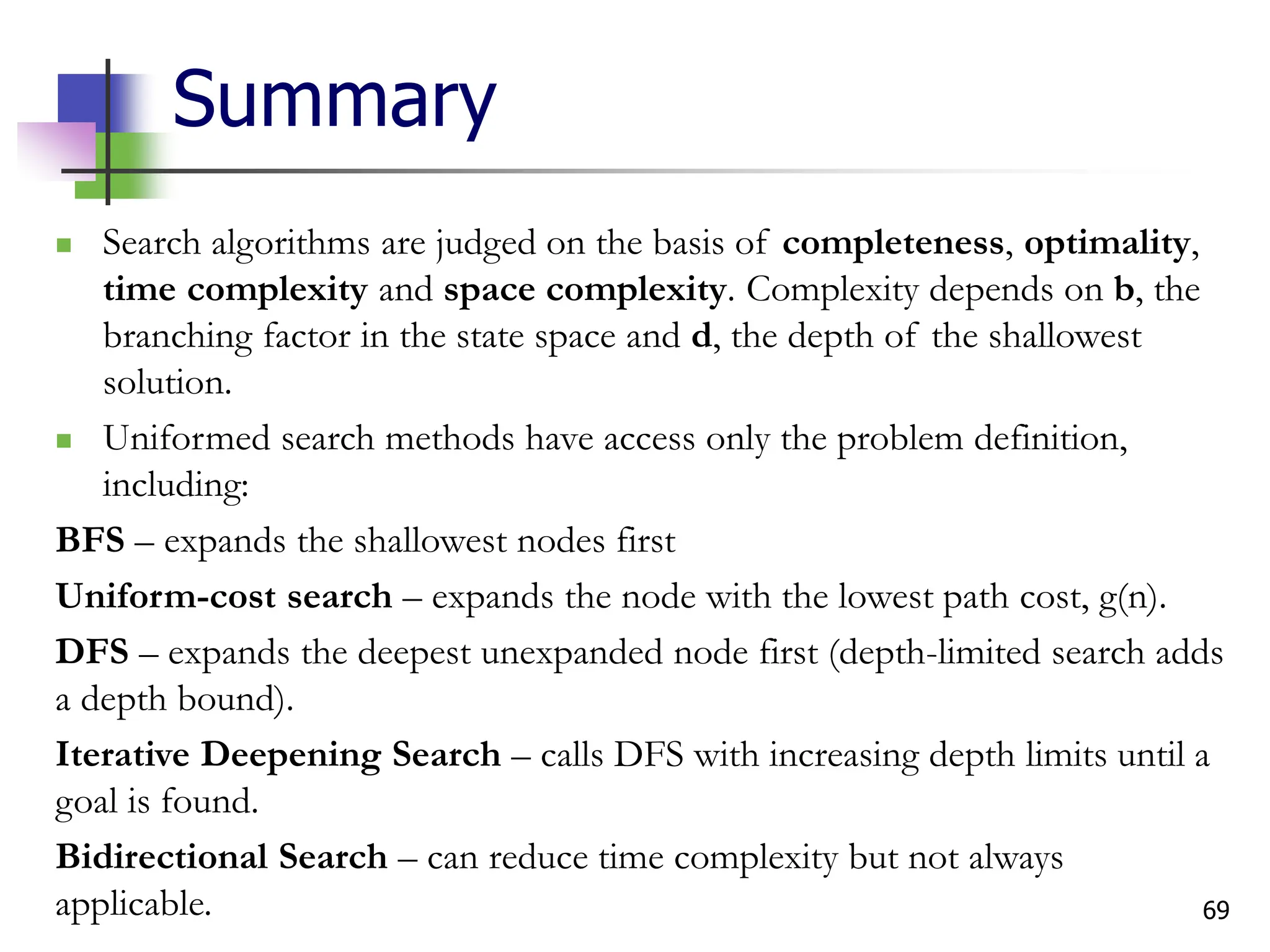
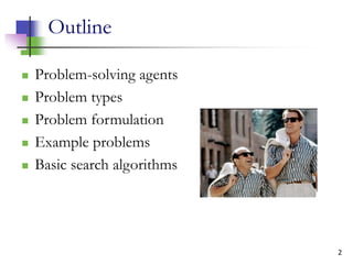
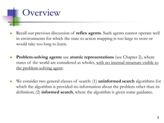
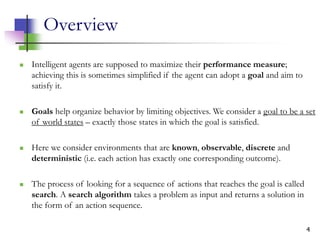
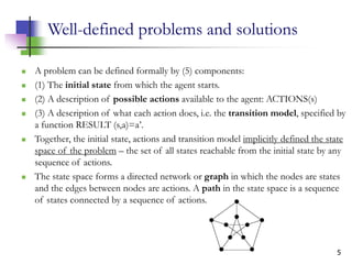
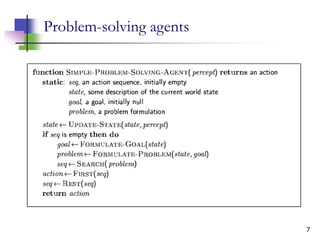
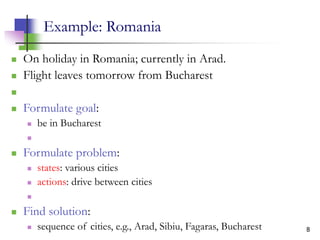
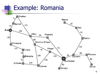
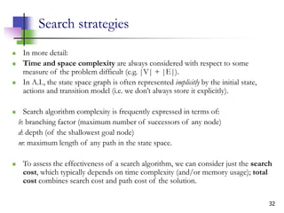
The document discusses problem-solving agents and search algorithms in artificial intelligence, outlining the components of well-defined problems and various types of searches, such as uninformed and informed search strategies. It illustrates example problems, like navigating from Arad to Bucharest, and outlines different problem types, including deterministic and nondeterministic scenarios. The text emphasizes the complexity of real-world state spaces and the importance of search algorithms in finding solutions efficiently.


![12
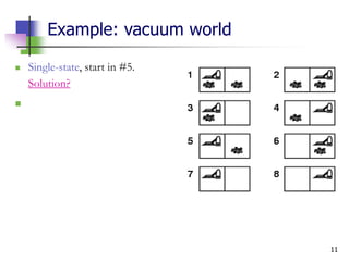
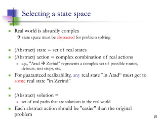
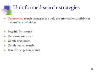
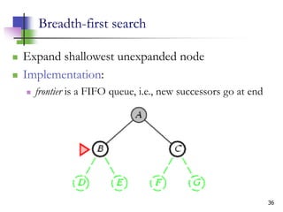
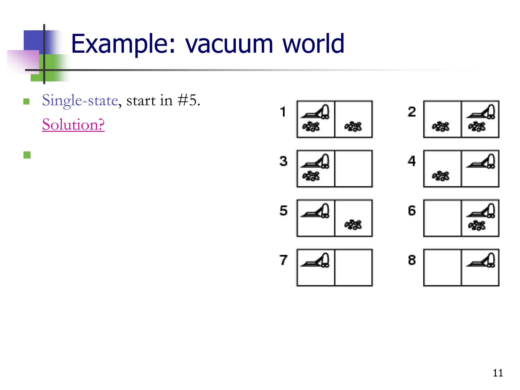
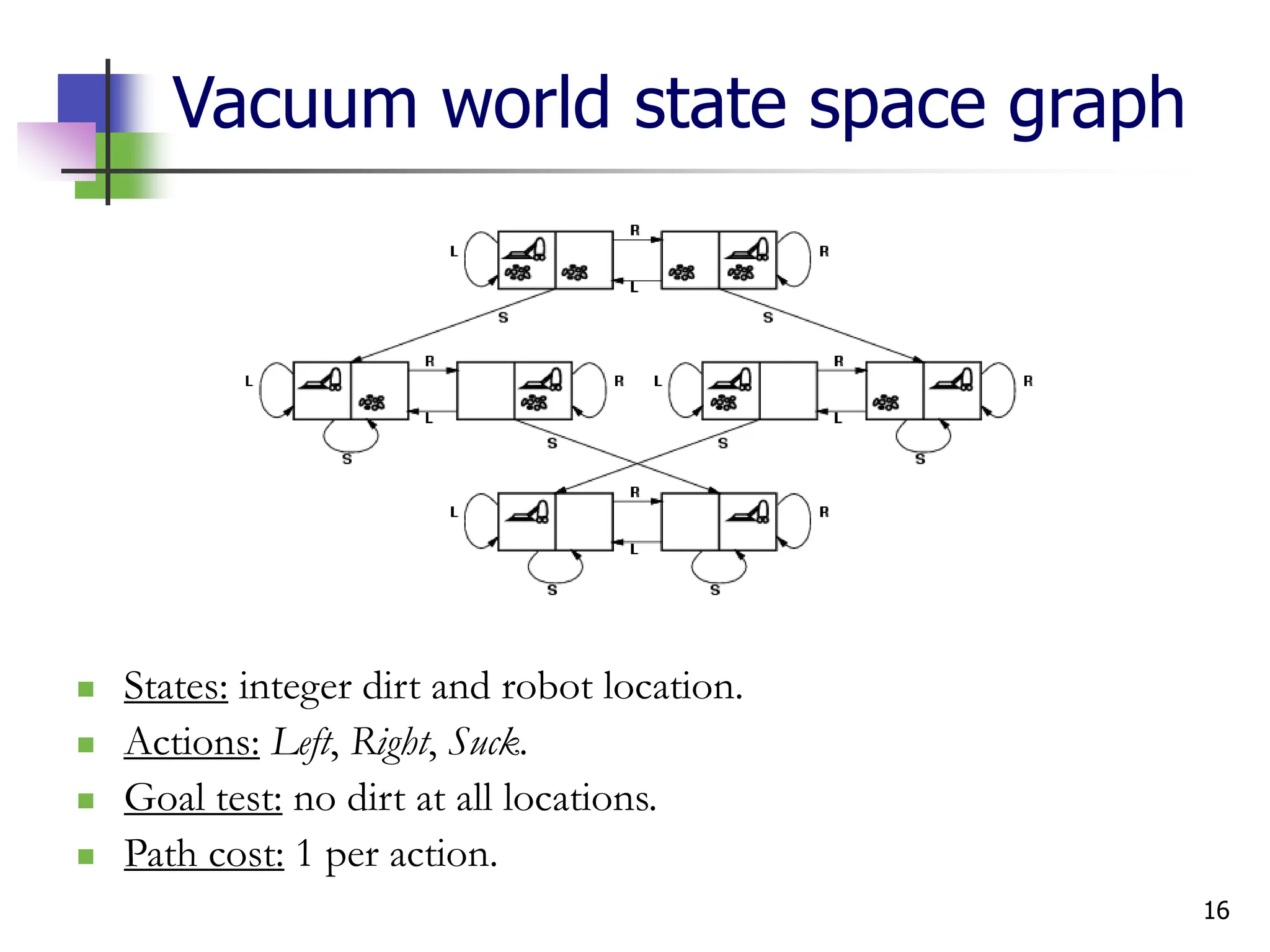
Example: vacuum world
Single-state, start in #5.
Solution? [Right, Suck]
Sensorless, start in
{1,2,3,4,5,6,7,8} e.g.,
Right goes to {2,4,6,8}
Solution?
](https://image.slidesharecdn.com/searchai-241213064213-1251b3a6/85/problem-solving-in-Artificial-intelligence-pdf-12-320.jpg)
![13
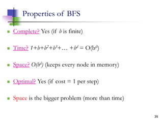
Example: vacuum world
Sensorless, start in
{1,2,3,4,5,6,7,8} e.g.,
Right goes to {2,4,6,8}
Solution?
[Right,Suck,Left,Suck]
Contingency
Nondeterministic: Suck may
dirty a clean carpet
Partially observable: location, dirt at current location.
Percept: [L, Clean], i.e., start in #5 or #7
Solution?](https://image.slidesharecdn.com/searchai-241213064213-1251b3a6/85/problem-solving-in-Artificial-intelligence-pdf-13-320.jpg)
![14
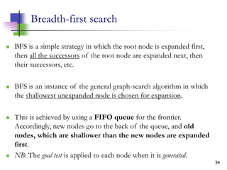
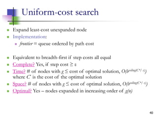
Example: vacuum world
Sensorless, start in
{1,2,3,4,5,6,7,8} e.g.,
Right goes to {2,4,6,8}
Solution?
[Right,Suck,Left,Suck]
Contingency
Nondeterministic: Suck may
dirty a clean carpet
Partially observable: location, dirt at current location.
Percept: [L, Clean], i.e., start in #5 or #7
Solution? [Right, if dirt then Suck]](https://image.slidesharecdn.com/searchai-241213064213-1251b3a6/85/problem-solving-in-Artificial-intelligence-pdf-14-320.jpg)
![17
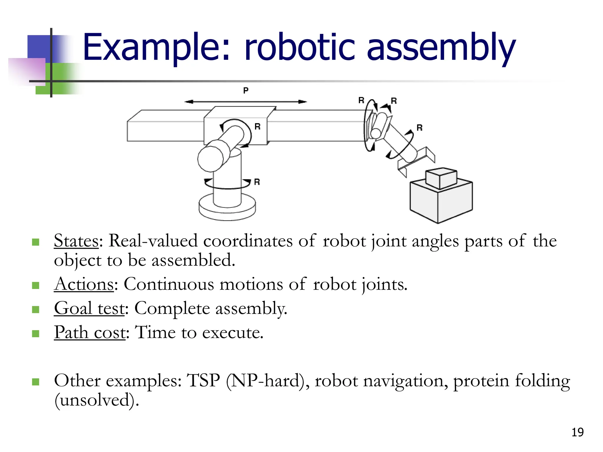
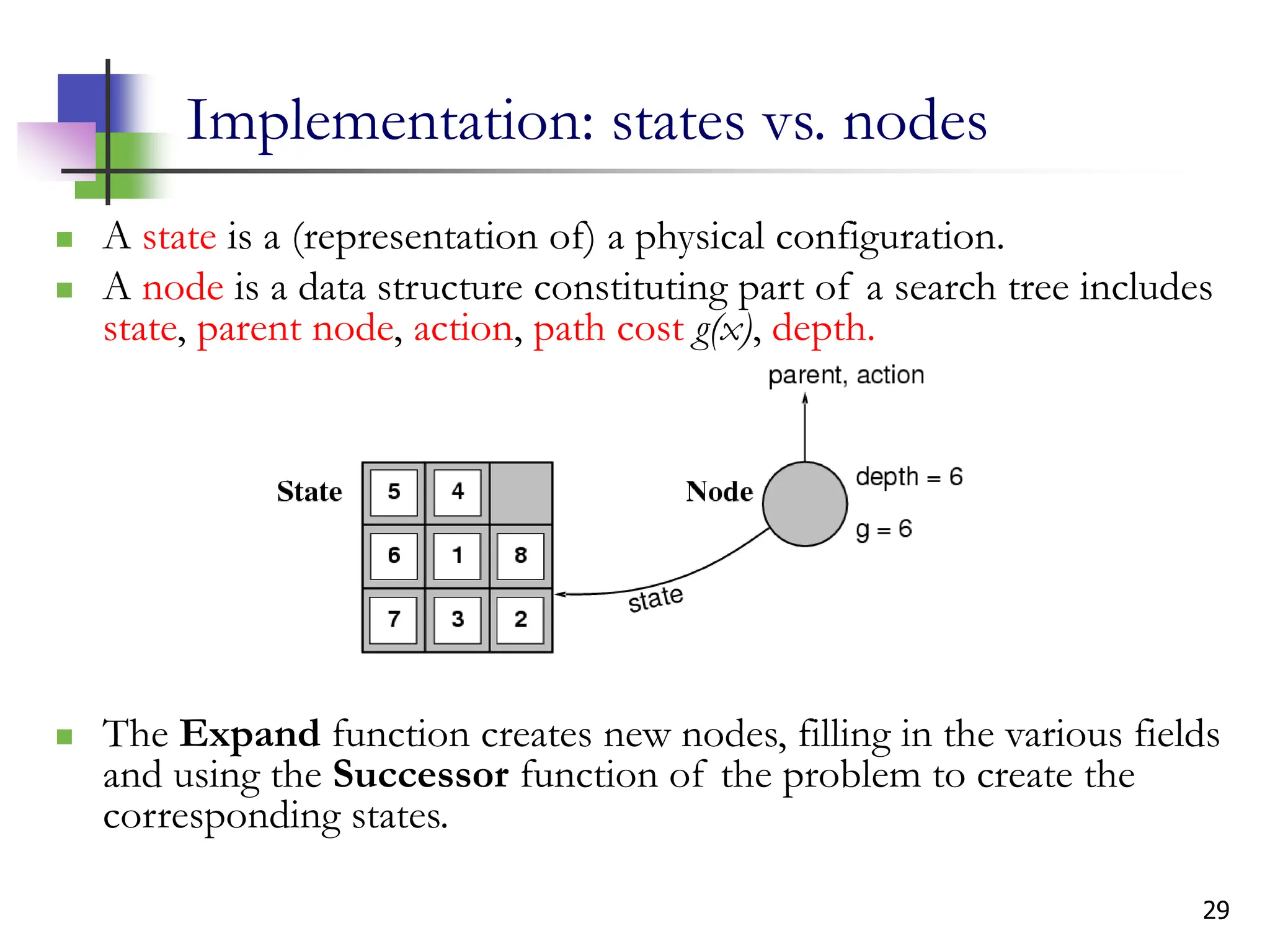
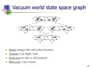
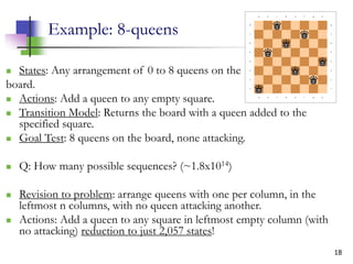
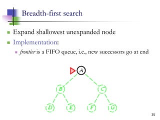
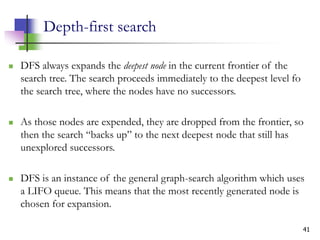
Example: The 8-puzzle
States: Locations of tiles. (Q: How large is state space?)
Actions: Move blank left, right, up, down.
Goal test: s==goal state. (given)
Path cost: 1 per move.
[Note: optimal solution of n-Puzzle family is NP-hard]](https://image.slidesharecdn.com/searchai-241213064213-1251b3a6/85/problem-solving-in-Artificial-intelligence-pdf-17-320.jpg)


![12
Example: vacuum world
Single-state, start in #5.
Solution? [Right, Suck]
Sensorless, start in
{1,2,3,4,5,6,7,8} e.g.,
Right goes to {2,4,6,8}
Solution?
](https://image.slidesharecdn.com/searchai-241213064213-1251b3a6/75/problem-solving-in-Artificial-intelligence-pdf-12-2048.jpg)
![13
Example: vacuum world
Sensorless, start in
{1,2,3,4,5,6,7,8} e.g.,
Right goes to {2,4,6,8}
Solution?
[Right,Suck,Left,Suck]
Contingency
Nondeterministic: Suck may
dirty a clean carpet
Partially observable: location, dirt at current location.
Percept: [L, Clean], i.e., start in #5 or #7
Solution?](https://image.slidesharecdn.com/searchai-241213064213-1251b3a6/75/problem-solving-in-Artificial-intelligence-pdf-13-2048.jpg)
![14
Example: vacuum world
Sensorless, start in
{1,2,3,4,5,6,7,8} e.g.,
Right goes to {2,4,6,8}
Solution?
[Right,Suck,Left,Suck]
Contingency
Nondeterministic: Suck may
dirty a clean carpet
Partially observable: location, dirt at current location.
Percept: [L, Clean], i.e., start in #5 or #7
Solution? [Right, if dirt then Suck]](https://image.slidesharecdn.com/searchai-241213064213-1251b3a6/75/problem-solving-in-Artificial-intelligence-pdf-14-2048.jpg)

![17
Example: The 8-puzzle
States: Locations of tiles. (Q: How large is state space?)
Actions: Move blank left, right, up, down.
Goal test: s==goal state. (given)
Path cost: 1 per move.
[Note: optimal solution of n-Puzzle family is NP-hard]](https://image.slidesharecdn.com/searchai-241213064213-1251b3a6/75/problem-solving-in-Artificial-intelligence-pdf-17-2048.jpg)