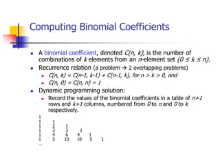
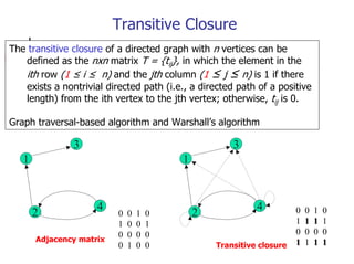
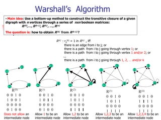
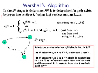
Dynamic programming is an algorithm design technique that solves problems by breaking them down into smaller overlapping subproblems and storing the solutions to subproblems to avoid recomputing them. It involves building up a solution using previously found subsolutions and working in a bottom-up fashion to solve larger subproblems from solutions to smaller subproblems. Examples where dynamic programming has been applied include computing Fibonacci numbers, finding the shortest paths in a graph, and solving optimization problems like the knapsack problem.


![Example: Fibonacci numbers
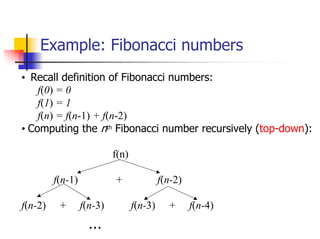
Computing the nth fibonacci number
using bottom-up iteration:
• f(0) = 0
• f(1) = 1
• f(2) = 0+1 = 1
• f(3) = 1+1 = 2
• f(4) = 1+2 = 3 ALGORITHM Fib(n)
• f(5) = 2+3 = 5 F[0] 0, F[1] 1
• for i 2 to n do
• F[i] F[i-1] + F[i-2]
• return F[n]
• f(n-2) =
• f(n-1) = extra space
• f(n) = f(n-1) + f(n-2)](https://image.slidesharecdn.com/s05cs303chap8-120411101334-phpapp01/85/Algorithm-chapter-8-4-320.jpg)


![The Knapsack Problem and Memory
Functions (1)
The problem
Find the most valuable subset of the given n
items that fit into a knapsack of capacity W.
Consider the following subproblem P(i, j)
Find the most valuable subset of the first i items
that fit into a knapsack of capacity j, where 1 ≤ i ≤
n, and 1≤ j ≤ W
Let V[i, j] be the value of an optimal solution to
the above subproblem P(i, j). Goal: V[n, W]
The question: What is the recurrence relation that
expresses a solution to this instance in terms of
solutions to smaller subinstances?](https://image.slidesharecdn.com/s05cs303chap8-120411101334-phpapp01/85/Algorithm-chapter-8-13-320.jpg)
![The Knapsack Problem and Memory
Functions (2)
The Recurrence
Two possibilities for the most valuable subset
for the subproblem P(i, j)
It does not include the ith item: V[i, j] = V[i-1, j]
It includes the ith item: V[i, j] = vi+ V[i-1, j – wi]
V[i, j] = max{V[i-1, j], vi+ V[i-1, j – wi] }, if j – wi ≥ 0
{ V[i-1, j] if j – wi < 0
V[0, j] = 0 for j ≥ 0 and V[i, 0] = 0 for i ≥ 0](https://image.slidesharecdn.com/s05cs303chap8-120411101334-phpapp01/85/Algorithm-chapter-8-14-320.jpg)
![Memory Functions
Memory functions: a combination of the top-down and bottom-
up method. The idea is to solve the subproblems that are
necessary and do it only once.
Top-down: solve common subproblems more than once.
Bottom-up: Solve subproblems whose solution are not necessary
for the solving the original problem.
ALGORITHM MFKnapsack(i, j)
if V[i, j] < 0 //if subproblem P(i, j) hasn’t been solved yet.
if j < Weights[i]
value MFKnapsack(i – 1, j)
else
value max(MFKnapsack(i – 1, j),
values[I] + MFKnapsck( i – 1, j – Weights[i]))
V[i, j] value
return V[i, j]](https://image.slidesharecdn.com/s05cs303chap8-120411101334-phpapp01/85/Algorithm-chapter-8-15-320.jpg)


![Example: Fibonacci numbers
Computing the nth fibonacci number
using bottom-up iteration:
• f(0) = 0
• f(1) = 1
• f(2) = 0+1 = 1
• f(3) = 1+1 = 2
• f(4) = 1+2 = 3 ALGORITHM Fib(n)
• f(5) = 2+3 = 5 F[0] 0, F[1] 1
• for i 2 to n do
• F[i] F[i-1] + F[i-2]
• return F[n]
• f(n-2) =
• f(n-1) = extra space
• f(n) = f(n-1) + f(n-2)](https://image.slidesharecdn.com/s05cs303chap8-120411101334-phpapp01/75/Algorithm-chapter-8-4-2048.jpg)


![The Knapsack Problem and Memory
Functions (1)
The problem
Find the most valuable subset of the given n
items that fit into a knapsack of capacity W.
Consider the following subproblem P(i, j)
Find the most valuable subset of the first i items
that fit into a knapsack of capacity j, where 1 ≤ i ≤
n, and 1≤ j ≤ W
Let V[i, j] be the value of an optimal solution to
the above subproblem P(i, j). Goal: V[n, W]
The question: What is the recurrence relation that
expresses a solution to this instance in terms of
solutions to smaller subinstances?](https://image.slidesharecdn.com/s05cs303chap8-120411101334-phpapp01/75/Algorithm-chapter-8-13-2048.jpg)
![The Knapsack Problem and Memory
Functions (2)
The Recurrence
Two possibilities for the most valuable subset
for the subproblem P(i, j)
It does not include the ith item: V[i, j] = V[i-1, j]
It includes the ith item: V[i, j] = vi+ V[i-1, j – wi]
V[i, j] = max{V[i-1, j], vi+ V[i-1, j – wi] }, if j – wi ≥ 0
{ V[i-1, j] if j – wi < 0
V[0, j] = 0 for j ≥ 0 and V[i, 0] = 0 for i ≥ 0](https://image.slidesharecdn.com/s05cs303chap8-120411101334-phpapp01/75/Algorithm-chapter-8-14-2048.jpg)
![Memory Functions
Memory functions: a combination of the top-down and bottom-
up method. The idea is to solve the subproblems that are
necessary and do it only once.
Top-down: solve common subproblems more than once.
Bottom-up: Solve subproblems whose solution are not necessary
for the solving the original problem.
ALGORITHM MFKnapsack(i, j)
if V[i, j] < 0 //if subproblem P(i, j) hasn’t been solved yet.
if j < Weights[i]
value MFKnapsack(i – 1, j)
else
value max(MFKnapsack(i – 1, j),
values[I] + MFKnapsck( i – 1, j – Weights[i]))
V[i, j] value
return V[i, j]](https://image.slidesharecdn.com/s05cs303chap8-120411101334-phpapp01/75/Algorithm-chapter-8-15-2048.jpg)


![UiPath Automation Suite Installation (Hands-On) [2/3]](https://cdn.slidesharecdn.com/ss_thumbnails/automationsuitecommunitysession2-251015095633-a6d862f1-thumbnail.jpg?width=600ounds&width=560&fit=bounds)


