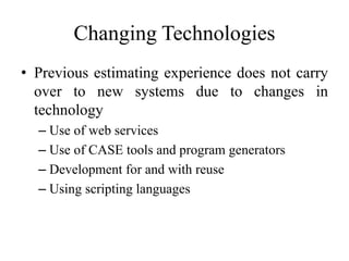
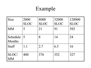
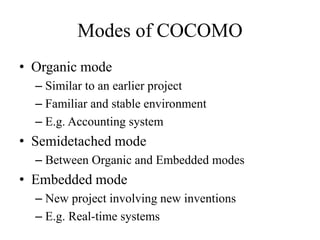
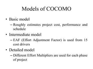
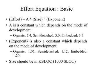
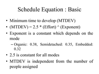
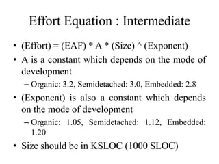
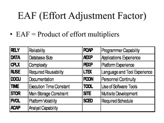
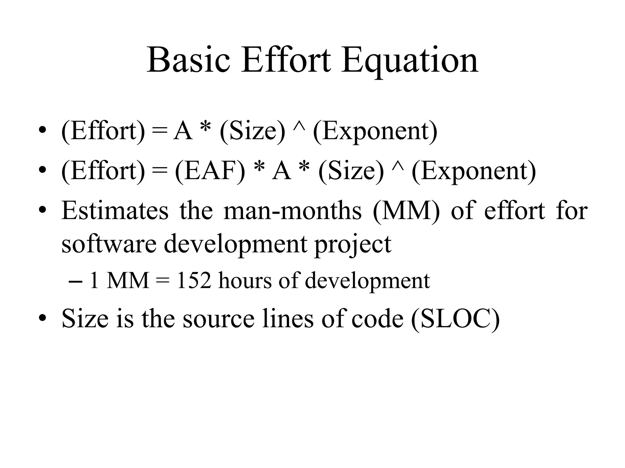
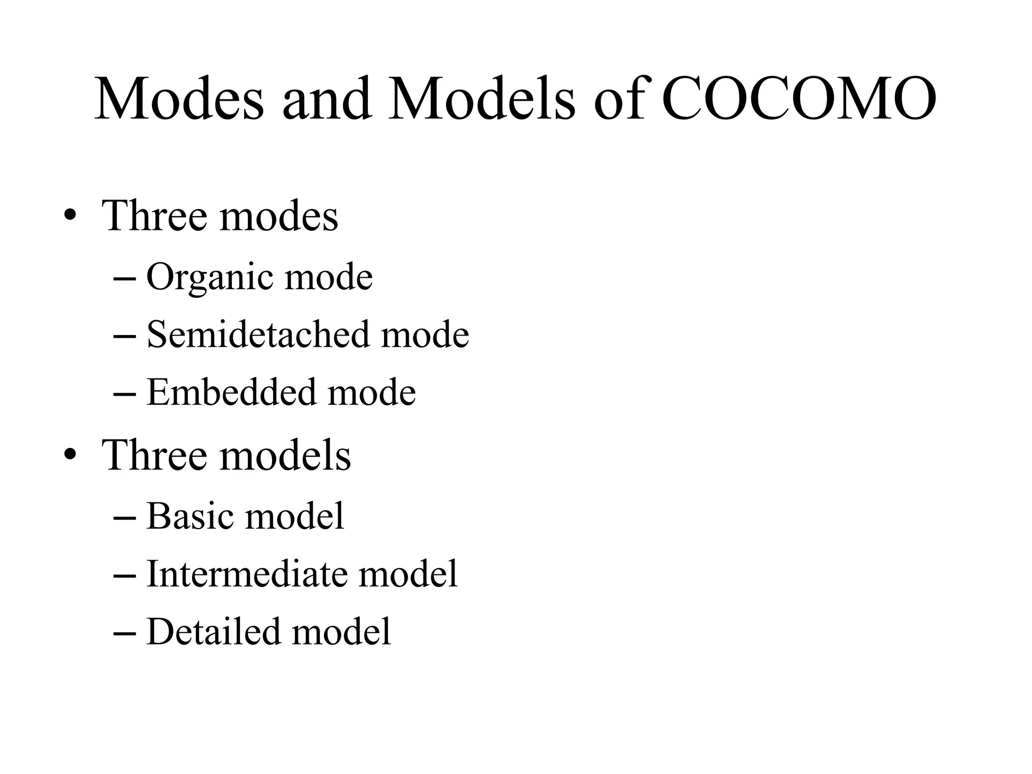
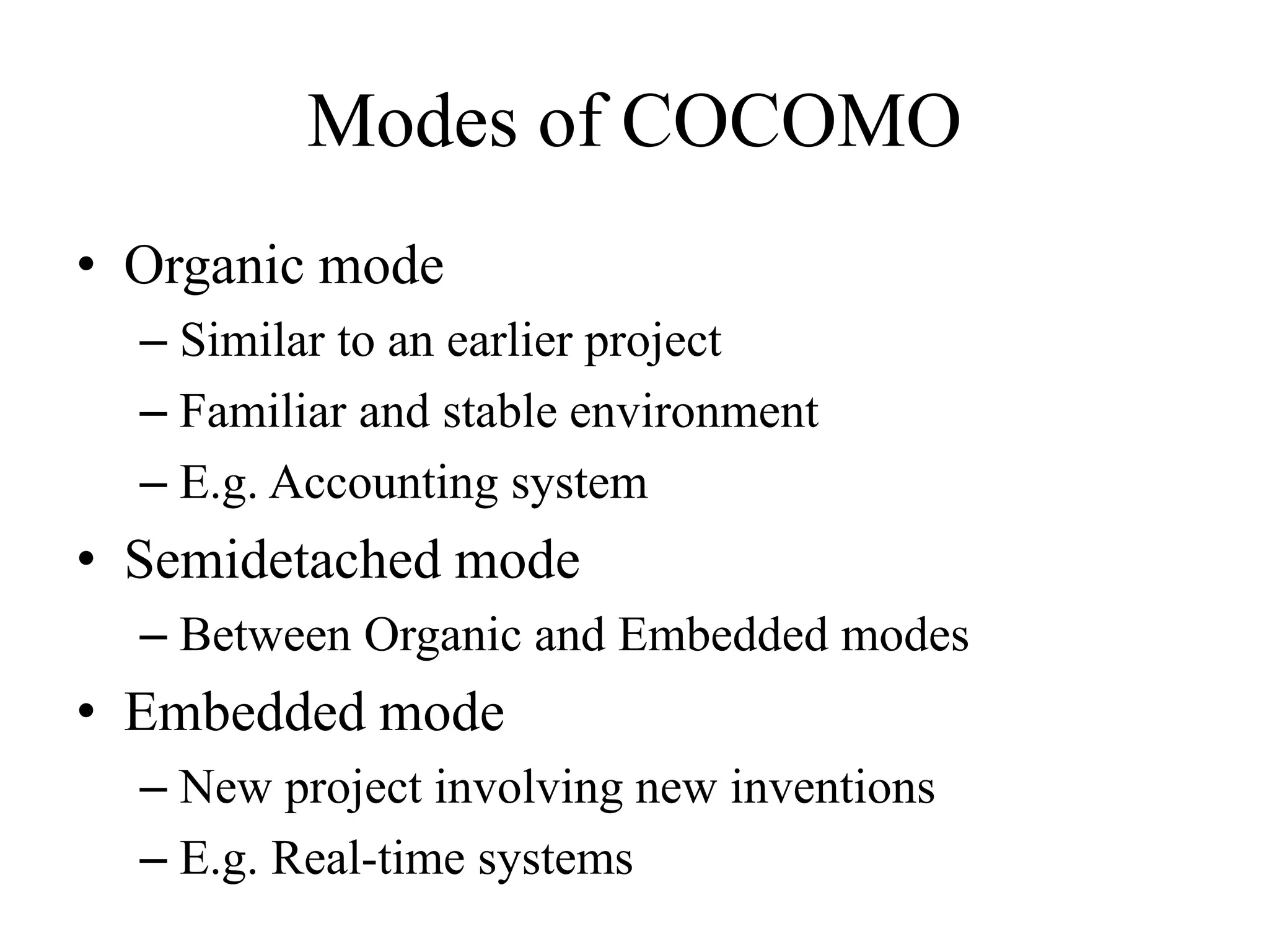
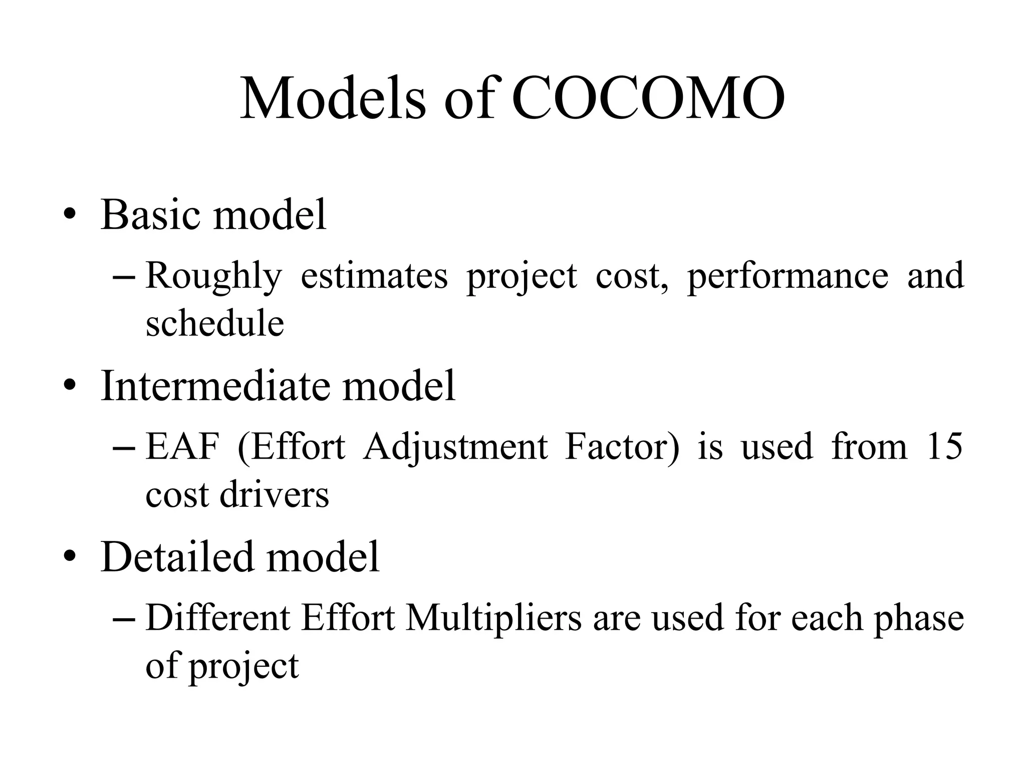
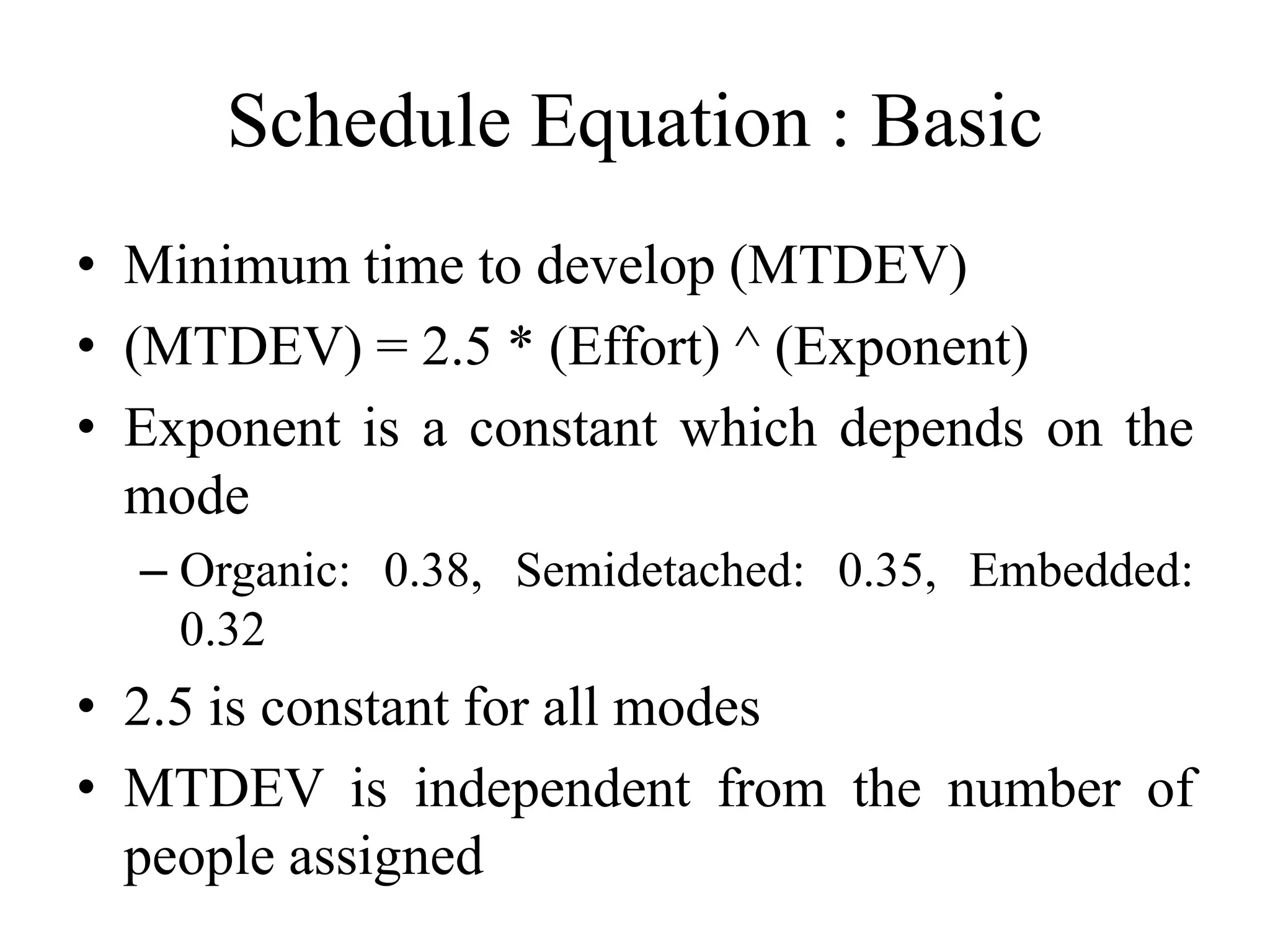
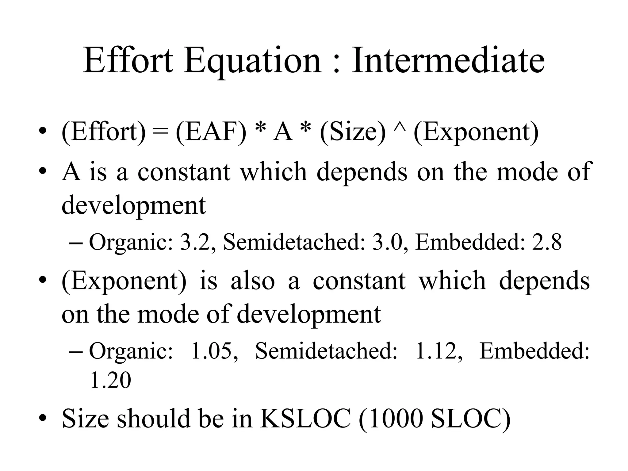
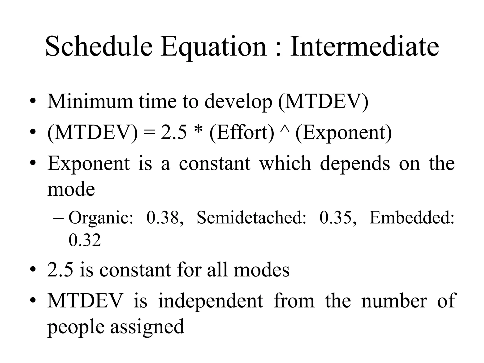
KEMBAR78
Algorithmic Software Cost Modeling | PPTX
Algorithmic Software Cost
Modeling
Kasun Ranga Wijeweera
(krw19870829@gmail.com)
Algorithmic Cost Modeling
• A mathematical function is used to estimate
the cost
– Inputs: Project, Process, Product
– Decided by project managers
• Historical data are studied to derive the
function
• Commonly used product attribute is LOC
(code size)
Software Productivity
• The rate at which individual software
engineers involve in development process is
known as software productivity
• Although quality assurance is a factor in
productivity assessment, the productivity is not
quality oriented
• The useful functionality produced per time unit
should be measured
Productivity Measures
• Size related measures:
– Lines of delivered source code
– Object code instructions
– Etc
• Function related measures:
– Functionality of the delivered software
– E.g. Function points
Lines of Code
• What programs should be considered as part of
the system?
• Assumption of the model:
– The relationship between system size and volume
of documentation is linear
• Key thing to remember:
– Uncertainty is more important than the initial line
– Seek justifiable bounds
Productivity Comparison
• Low level language verses high level language
• Verbose code verses compact code
Function Points
• Program characteristics are considered
– External inputs and outputs
– User interactions
– External interfaces
– Files used by the system
• Corresponding weights are assigned to each
characteristic
FPs and LOC
• FPs can be used to estimate LOC
– LOC = AVC * (Number of FPs)
– AVC is a factor which depends on the
programming language
• Assembly language: AVC = 200 to 300
• 4 GL language: AVC = 2 to 40
• FPs are subjective and dependent on the
estimator
– FP automation is impossible
Productivity Estimates
• Real time embedded systems
– 40 to 60 LOC per month
• Systems programs
– 150 to 400 LOC per month
• Commercial applications
– 200 to 900 LOC per month
Productivity Factors
• Application domain experience
• Process quality
• Product size
• Technology support
• Working environment
Changing Technologies
• Previous estimating experience does not carry
over to new systems due to changes in
technology
– Use of web services
– Use of CASE tools and program generators
– Development for and with reuse
– Using scripting languages
COCOMO
• Constructive Cost Model (COCOMO)
• Estimates are derived as functions of variables
• Data of past projects must be available
• First published by Dr. Barry Boehm in 1981
• Derived through statistical regression of data
from 63 past projects
Example
Size 2000
SLOC
8000
SLOC
32000
SLOC
128000
SLOC
MM 5 21 91 392
Schedule
Months
5 8 14 24
Staff 1.1 2.7 6.5 16
SLOC/
MM
400 376 352 327
Basic Effort Equation
• (Effort) = A * (Size) ^ (Exponent)
• (Effort) = (EAF) * A * (Size) ^ (Exponent)
• Estimates the man-months (MM) of effort for
software development project
– 1 MM = 152 hours of development
• Size is the source lines of code (SLOC)
Modes and Models of COCOMO
• Three modes
– Organic mode
– Semidetached mode
– Embedded mode
• Three models
– Basic model
– Intermediate model
– Detailed model
Modes of COCOMO
• Organic mode
– Similar to an earlier project
– Familiar and stable environment
– E.g. Accounting system
• Semidetached mode
– Between Organic and Embedded modes
• Embedded mode
– New project involving new inventions
– E.g. Real-time systems
Models of COCOMO
• Basic model
– Roughly estimates project cost, performance and
schedule
• Intermediate model
– EAF (Effort Adjustment Factor) is used from 15
cost drivers
• Detailed model
– Different Effort Multipliers are used for each phase
of project
Effort Equation : Basic
• (Effort) = A * (Size) ^ (Exponent)
• A is a constant which depends on the mode of
development
– Organic: 2.4, Semidetached: 3.0, Embedded: 3.6
• (Exponent) is also a constant which depends
on the mode of development
– Organic: 1.05, Semidetached: 1.12, Embedded:
1.20
• Size should be in KSLOC (1000 SLOC)
Schedule Equation : Basic
• Minimum time to develop (MTDEV)
• (MTDEV) = 2.5 * (Effort) ^ (Exponent)
• Exponent is a constant which depends on the
mode
– Organic: 0.38, Semidetached: 0.35, Embedded:
0.32
• 2.5 is constant for all modes
• MTDEV is independent from the number of
people assigned
Effort Equation : Intermediate
• (Effort) = (EAF) * A * (Size) ^ (Exponent)
• A is a constant which depends on the mode of
development
– Organic: 3.2, Semidetached: 3.0, Embedded: 2.8
• (Exponent) is also a constant which depends
on the mode of development
– Organic: 1.05, Semidetached: 1.12, Embedded:
1.20
• Size should be in KSLOC (1000 SLOC)
EAF (Effort Adjustment Factor)
• EAF = Product of effort multipliers
Schedule Equation : Intermediate
• Minimum time to develop (MTDEV)
• (MTDEV) = 2.5 * (Effort) ^ (Exponent)
• Exponent is a constant which depends on the
mode
– Organic: 0.38, Semidetached: 0.35, Embedded:
0.32
• 2.5 is constant for all modes
• MTDEV is independent from the number of
people assigned
Tool Demonstration
http://sunset.usc.edu/research/COCOMOII/expert_co
como/expert_cocomo2000.html
Thank you!

Algorithmic Software Cost Modeling

  • 1.
    Algorithmic Software Cost Modeling KasunRanga Wijeweera (krw19870829@gmail.com)
  • 2.
    Algorithmic Cost Modeling •A mathematical function is used to estimate the cost – Inputs: Project, Process, Product – Decided by project managers • Historical data are studied to derive the function • Commonly used product attribute is LOC (code size)
  • 3.
    Software Productivity • Therate at which individual software engineers involve in development process is known as software productivity • Although quality assurance is a factor in productivity assessment, the productivity is not quality oriented • The useful functionality produced per time unit should be measured
  • 4.
    Productivity Measures • Sizerelated measures: – Lines of delivered source code – Object code instructions – Etc • Function related measures: – Functionality of the delivered software – E.g. Function points
  • 5.
    Lines of Code •What programs should be considered as part of the system? • Assumption of the model: – The relationship between system size and volume of documentation is linear • Key thing to remember: – Uncertainty is more important than the initial line – Seek justifiable bounds
  • 6.
    Productivity Comparison • Lowlevel language verses high level language • Verbose code verses compact code
  • 7.
    Function Points • Programcharacteristics are considered – External inputs and outputs – User interactions – External interfaces – Files used by the system • Corresponding weights are assigned to each characteristic
  • 8.
    FPs and LOC •FPs can be used to estimate LOC – LOC = AVC * (Number of FPs) – AVC is a factor which depends on the programming language • Assembly language: AVC = 200 to 300 • 4 GL language: AVC = 2 to 40 • FPs are subjective and dependent on the estimator – FP automation is impossible
  • 9.
    Productivity Estimates • Realtime embedded systems – 40 to 60 LOC per month • Systems programs – 150 to 400 LOC per month • Commercial applications – 200 to 900 LOC per month
  • 10.
    Productivity Factors • Applicationdomain experience • Process quality • Product size • Technology support • Working environment
  • 11.
    Changing Technologies • Previousestimating experience does not carry over to new systems due to changes in technology – Use of web services – Use of CASE tools and program generators – Development for and with reuse – Using scripting languages
  • 12.
    COCOMO • Constructive CostModel (COCOMO) • Estimates are derived as functions of variables • Data of past projects must be available • First published by Dr. Barry Boehm in 1981 • Derived through statistical regression of data from 63 past projects
  • 13.
    Example Size 2000 SLOC 8000 SLOC 32000 SLOC 128000 SLOC MM 521 91 392 Schedule Months 5 8 14 24 Staff 1.1 2.7 6.5 16 SLOC/ MM 400 376 352 327
  • 14.
    Basic Effort Equation •(Effort) = A * (Size) ^ (Exponent) • (Effort) = (EAF) * A * (Size) ^ (Exponent) • Estimates the man-months (MM) of effort for software development project – 1 MM = 152 hours of development • Size is the source lines of code (SLOC)
  • 15.
    Modes and Modelsof COCOMO • Three modes – Organic mode – Semidetached mode – Embedded mode • Three models – Basic model – Intermediate model – Detailed model
  • 16.
    Modes of COCOMO •Organic mode – Similar to an earlier project – Familiar and stable environment – E.g. Accounting system • Semidetached mode – Between Organic and Embedded modes • Embedded mode – New project involving new inventions – E.g. Real-time systems
  • 17.
    Models of COCOMO •Basic model – Roughly estimates project cost, performance and schedule • Intermediate model – EAF (Effort Adjustment Factor) is used from 15 cost drivers • Detailed model – Different Effort Multipliers are used for each phase of project
  • 18.
    Effort Equation :Basic • (Effort) = A * (Size) ^ (Exponent) • A is a constant which depends on the mode of development – Organic: 2.4, Semidetached: 3.0, Embedded: 3.6 • (Exponent) is also a constant which depends on the mode of development – Organic: 1.05, Semidetached: 1.12, Embedded: 1.20 • Size should be in KSLOC (1000 SLOC)
  • 19.
    Schedule Equation :Basic • Minimum time to develop (MTDEV) • (MTDEV) = 2.5 * (Effort) ^ (Exponent) • Exponent is a constant which depends on the mode – Organic: 0.38, Semidetached: 0.35, Embedded: 0.32 • 2.5 is constant for all modes • MTDEV is independent from the number of people assigned
  • 20.
    Effort Equation :Intermediate • (Effort) = (EAF) * A * (Size) ^ (Exponent) • A is a constant which depends on the mode of development – Organic: 3.2, Semidetached: 3.0, Embedded: 2.8 • (Exponent) is also a constant which depends on the mode of development – Organic: 1.05, Semidetached: 1.12, Embedded: 1.20 • Size should be in KSLOC (1000 SLOC)
  • 21.
    EAF (Effort AdjustmentFactor) • EAF = Product of effort multipliers
  • 22.
    Schedule Equation :Intermediate • Minimum time to develop (MTDEV) • (MTDEV) = 2.5 * (Effort) ^ (Exponent) • Exponent is a constant which depends on the mode – Organic: 0.38, Semidetached: 0.35, Embedded: 0.32 • 2.5 is constant for all modes • MTDEV is independent from the number of people assigned
  • 23.
  • 24.