1. An algorithm is a sequence of unambiguous instructions to solve a problem and obtain an output for any valid input in a finite amount of time. Pseudocode is used to describe algorithms using a natural language format.
2. Analyzing algorithm efficiency involves determining the theoretical and empirical time complexity by counting the number of basic operations performed relative to the input size. Common measures are best-case, worst-case, average-case, and amortized analysis.
3. Important problem types for algorithms include sorting, searching, string processing, graphs, combinatorics, geometry, and numerical problems. Fundamental algorithms are analyzed for correctness and time/space complexity.
Overview of algorithm design and analysis, including definition and structure. Introduction to pseudocode, formatting, and key terminologies used in algorithm design. Explanation of the Sieve of Eratosthenes for generating prime numbers. Fundamental principles in formulating algorithms and problem-solving methodologies.
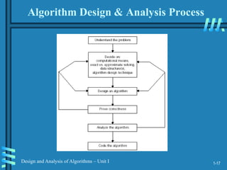
Eight steps of algorithm design including problem understanding, capability ascertaining, and proving correctness.
1-1
Design and Analysisof Algorithms – Unit I
Algorithm
An Algorithm is a sequence of unambiguous
instructions for solving a problem,
i.e., for obtaining a required output for any
legitimate input in a finite amount of time.
3.
1-2
Design and Analysisof Algorithms – Unit I
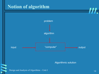
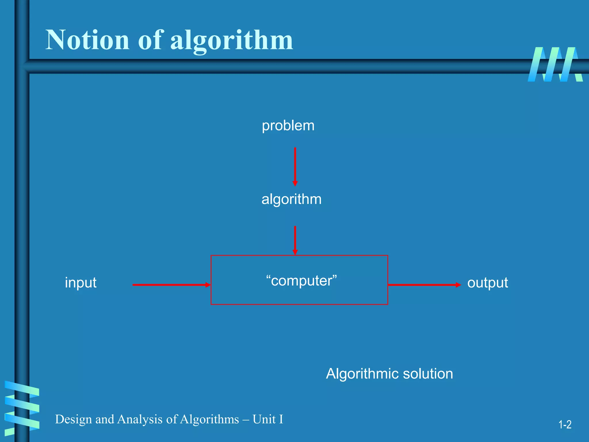
Notion of algorithm
“computer”
Algorithmic solution
problem
algorithm
input output
4.
1-3
Design and Analysisof Algorithms – Unit I
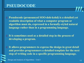
PSEUDOCODE
Pseudocode (pronounced SOO-doh-kohd) is a detailed yet
readable description of what a computer program or
algorithm must do, expressed in a formally-styled natural
language rather than in a programming language.
It is sometimes used as a detailed step in the process of
developing a program.
It allows programmers to express the design in great detail
and provides programmers a detailed template for the next
step of writing code in a specific programming language.
5.
1-4
Design and Analysisof Algorithms – Unit I
Formatting and Conventions in Pseudocoding
INDENTATION in pseudocode should be identical to its
implementation in a programming language. Try to indent
at least four spaces.
The pseudocode entries are to be cryptic, AND SHOULD
NOT BE PROSE. NO SENTENCES.
No flower boxes in pseudocode.
Do not include data declarations in pseudocode.
6.
1-5
Design and Analysisof Algorithms – Unit I
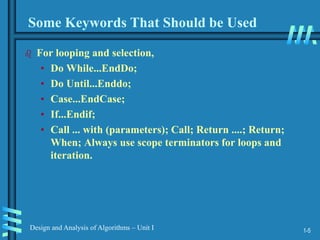
Some Keywords That Should be Used
For looping and selection,
• Do While...EndDo;
• Do Until...Enddo;
• Case...EndCase;
• If...Endif;
• Call ... with (parameters); Call; Return ....; Return;
When; Always use scope terminators for loops and
iteration.
7.
1-6
Design and Analysisof Algorithms – Unit I
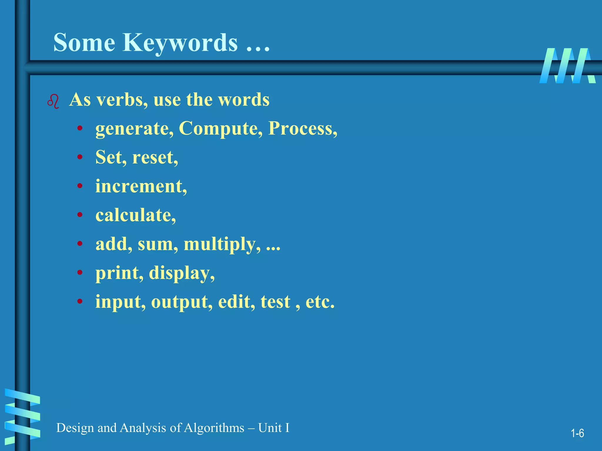
Some Keywords …
As verbs, use the words
• generate, Compute, Process,
• Set, reset,
• increment,
• calculate,
• add, sum, multiply, ...
• print, display,
• input, output, edit, test , etc.
1-8
Design and Analysisof Algorithms – Unit I
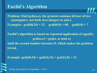
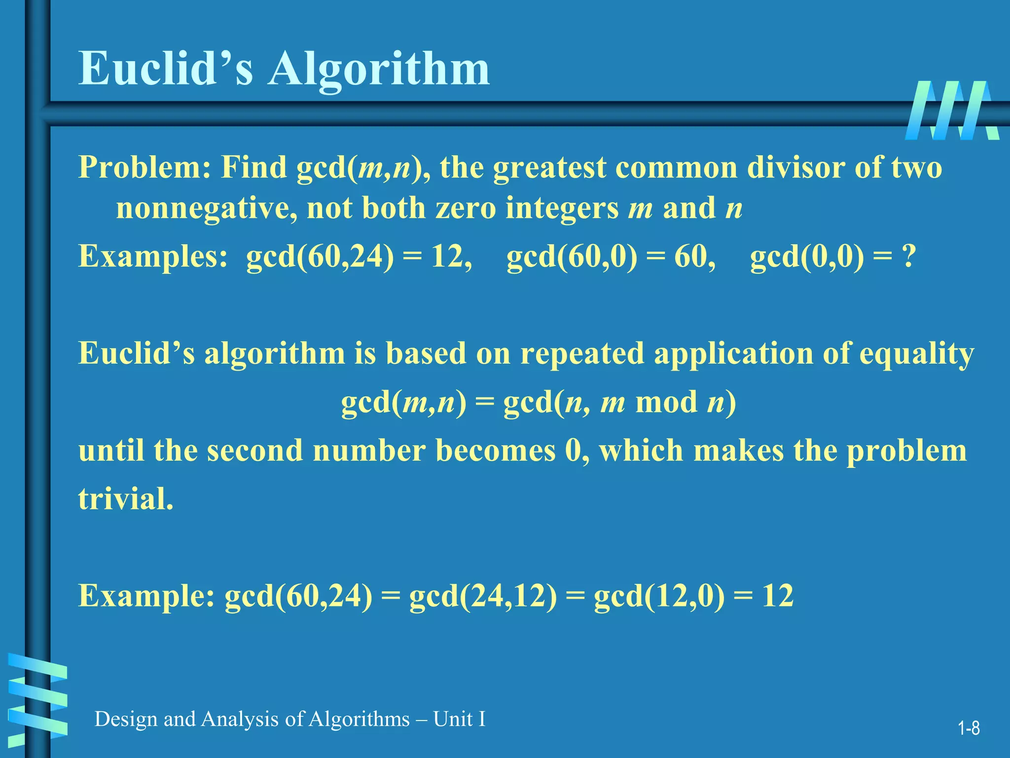
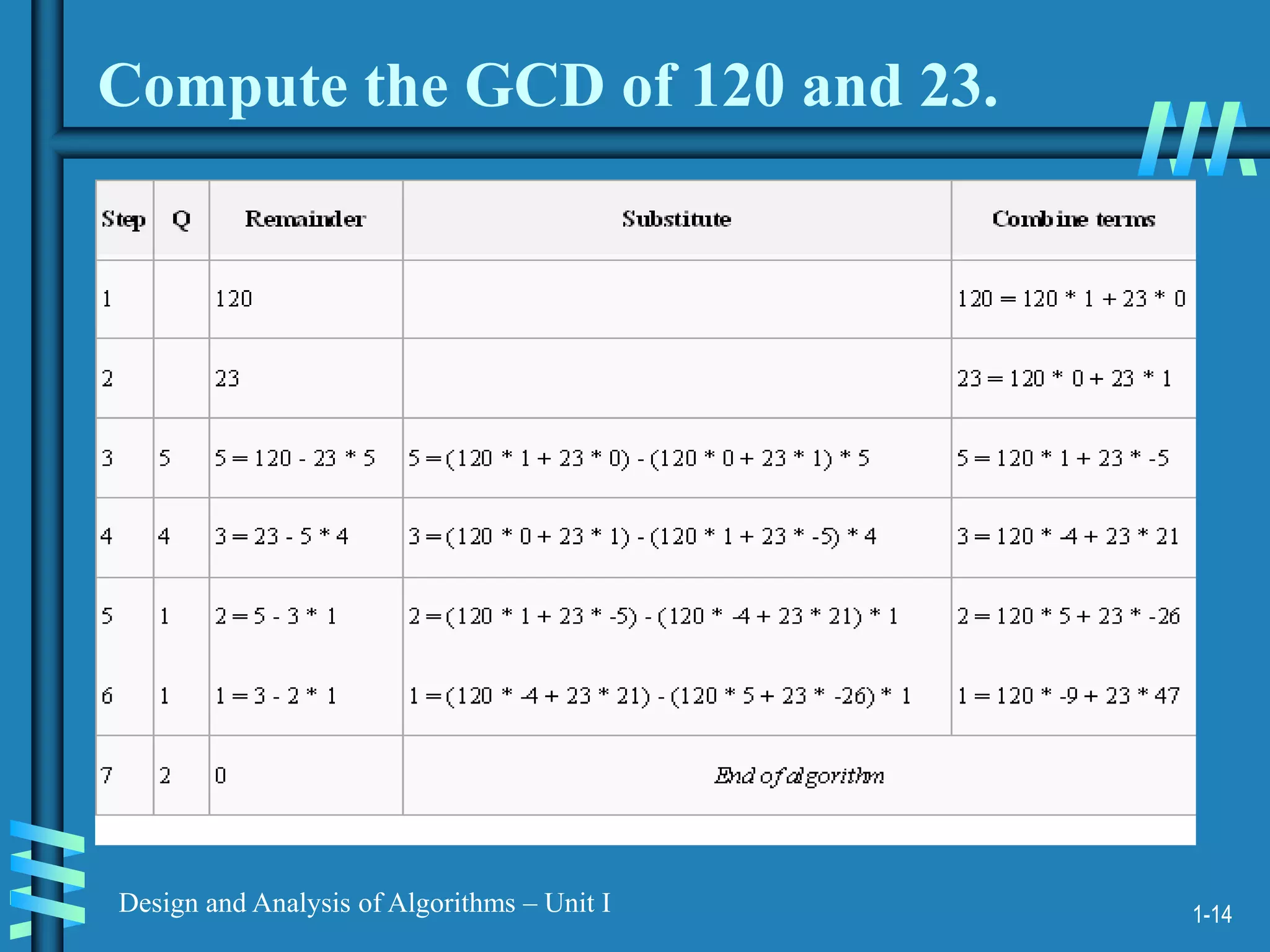
Euclid’s Algorithm
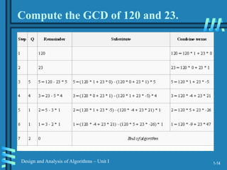
Problem: Find gcd(m,n), the greatest common divisor of two
nonnegative, not both zero integers m and n
Examples: gcd(60,24) = 12, gcd(60,0) = 60, gcd(0,0) = ?
Euclid’s algorithm is based on repeated application of equality
gcd(m,n) = gcd(n, m mod n)
until the second number becomes 0, which makes the problem
trivial.
Example: gcd(60,24) = gcd(24,12) = gcd(12,0) = 12
10.
1-9
Design and Analysisof Algorithms – Unit I
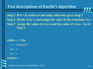
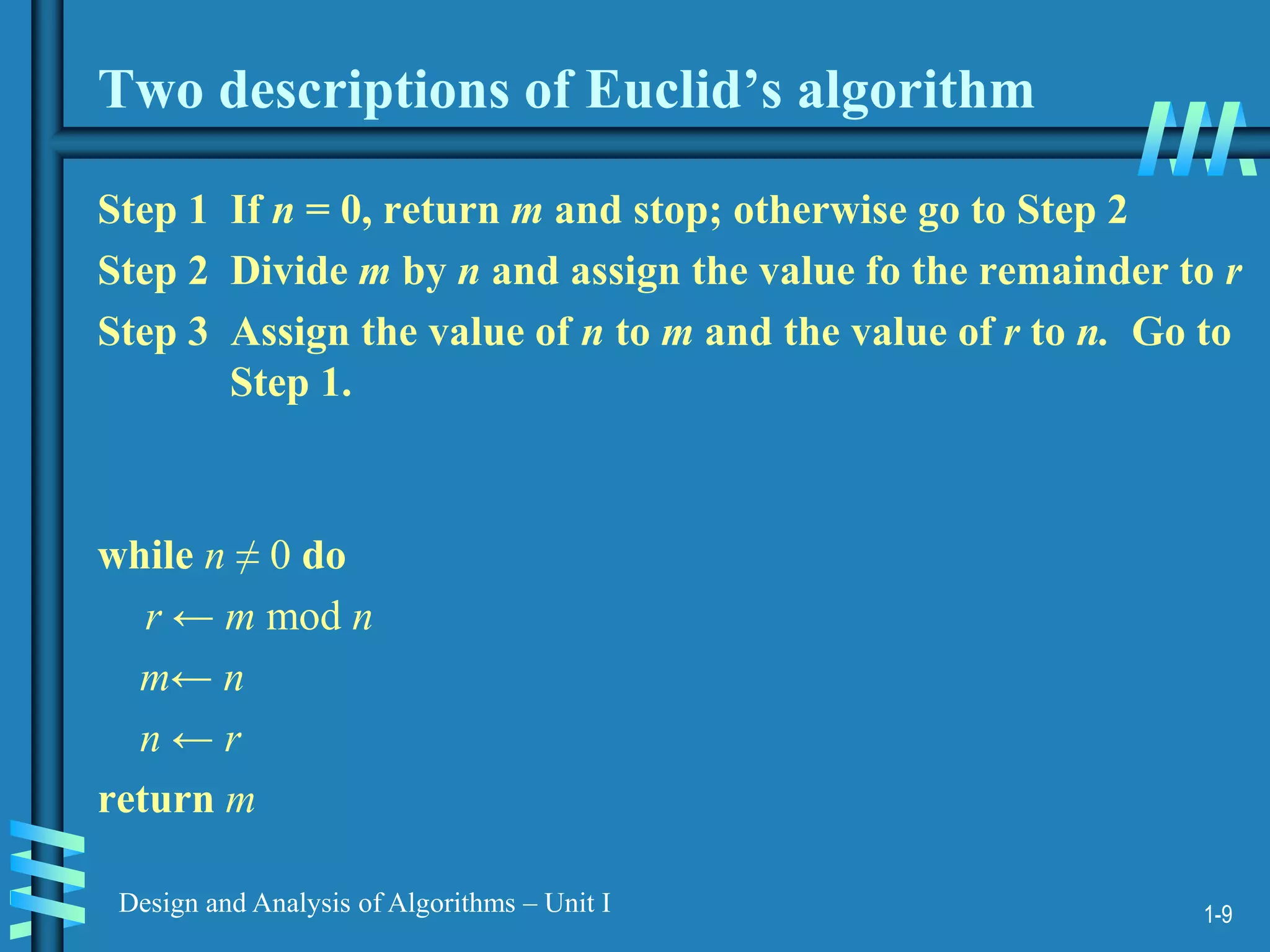
Two descriptions of Euclid’s algorithm
Step 1 If n = 0, return m and stop; otherwise go to Step 2
Step 2 Divide m by n and assign the value fo the remainder to r
Step 3 Assign the value of n to m and the value of r to n. Go to
Step 1.
while n ≠ 0 do
r ← m mod n
m← n
n ← r
return m
11.
1-10
Design and Analysisof Algorithms – Unit I
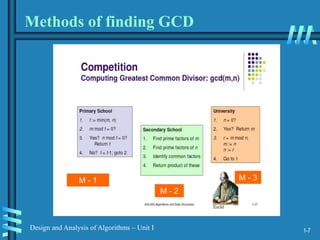
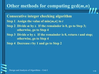
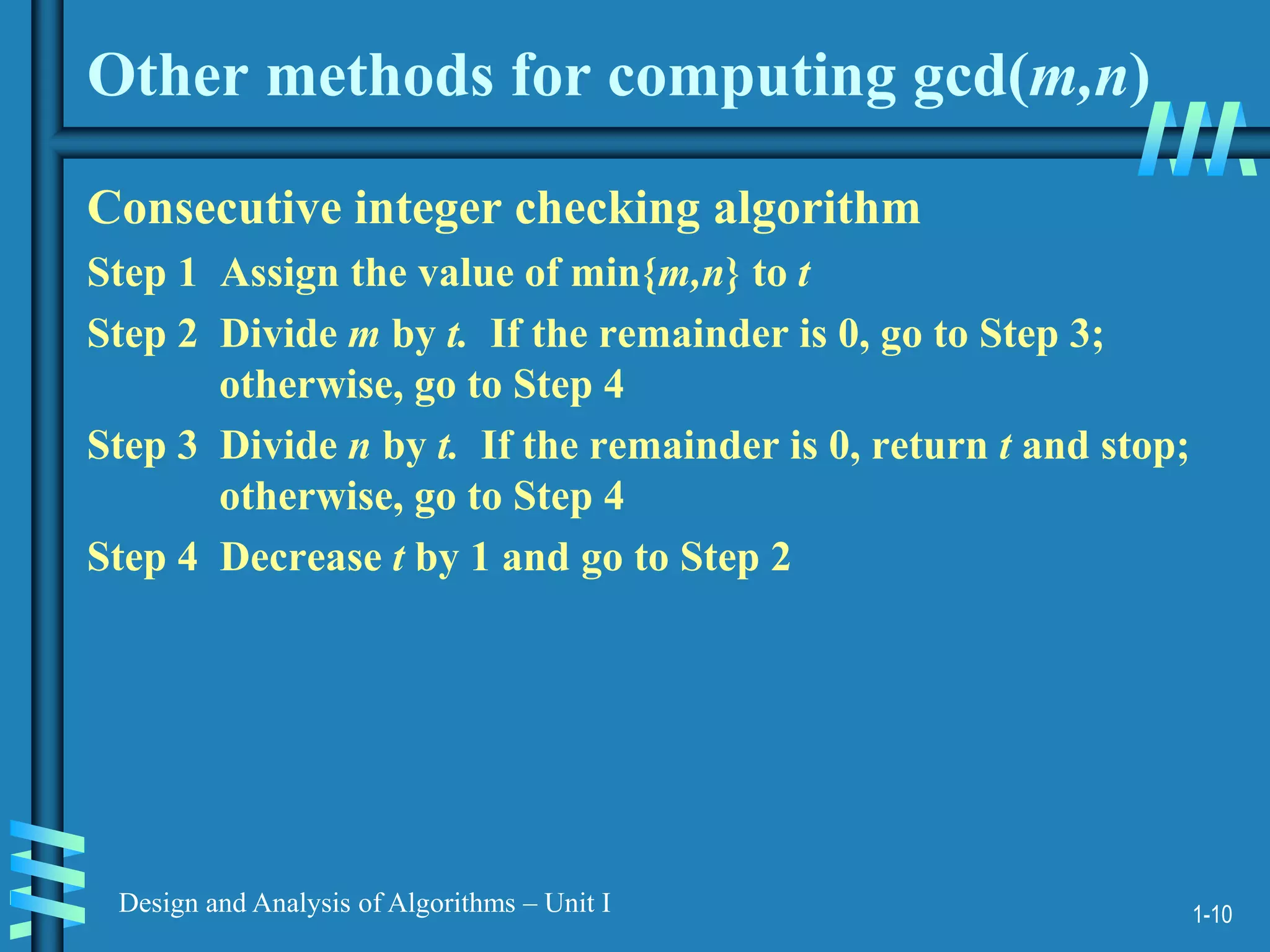
Other methods for computing gcd(m,n)
Consecutive integer checking algorithm
Step 1 Assign the value of min{m,n} to t
Step 2 Divide m by t. If the remainder is 0, go to Step 3;
otherwise, go to Step 4
Step 3 Divide n by t. If the remainder is 0, return t and stop;
otherwise, go to Step 4
Step 4 Decrease t by 1 and go to Step 2
12.
1-11
Design and Analysisof Algorithms – Unit I
Other methods for gcd(m,n) [cont.]
Middle-school procedure
Step 1 Find the prime factorization of m
Step 2 Find the prime factorization of n
Step 3 Find all the common prime factors
Step 4 Compute the product of all the common prime factors
and return it as gcd(m,n)
Is this an algorithm?
13.
1-12
Design and Analysisof Algorithms – Unit I
Sieve of Eratosthenes
Input: Integer n ≥ 2
Output: List of primes less than or equal to n
for p ← 2 to n do A[p] ← p
for p ← 2 to n do
if A[p] 0 //p hasn’t been previously eliminated from the list
j ← p* p
while j ≤ n do
A[j] ← 0 //mark element as eliminated
j ← j + p
Example: 2 3 4 5 6 7 8 9 10 11 12 13 14 15 16 17 18 19 20
14.
1-13
Design and Analysisof Algorithms – Unit I
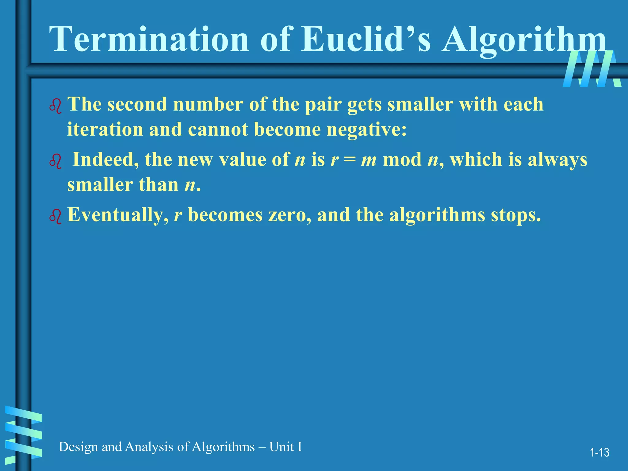
Termination of Euclid’s Algorithm
The second number of the pair gets smaller with each
iteration and cannot become negative:
Indeed, the new value of n is r = m mod n, which is always
smaller than n.
Eventually, r becomes zero, and the algorithms stops.
1-16
Design and Analysisof Algorithms – Unit I
Fundamentals of Algorithmic Problem
Solving
Algorithm = Procedural Solutions to Problem
NOT an answer, BUT rather specific instructions of
getting answers.
Therefore, requires steps in designing and analyzing an
algorithm
1-18
Design and Analysisof Algorithms – Unit I
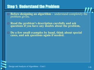
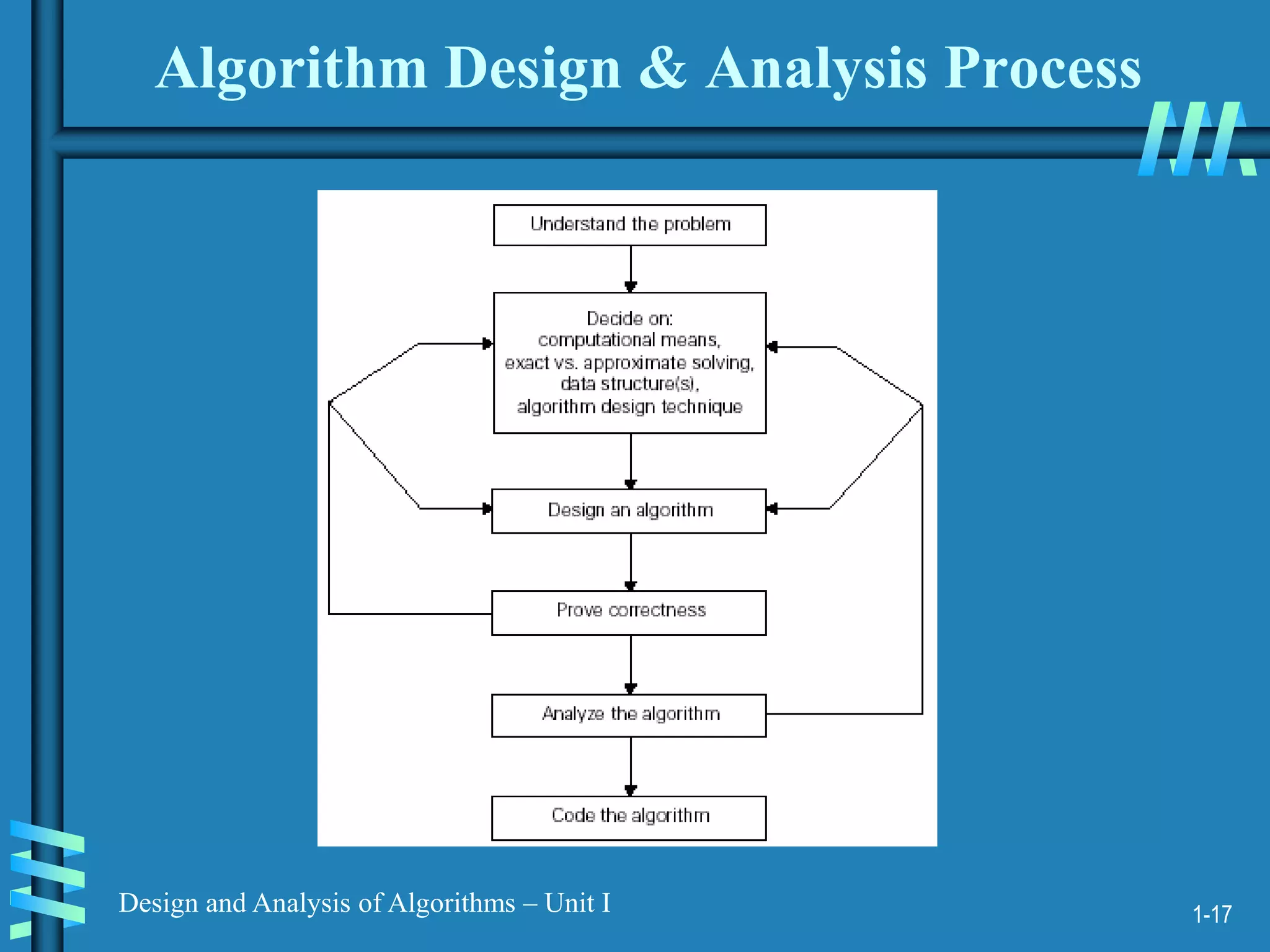
Step 1: Understand the Problem
Before designing an algorithm - understand completely the
problem given.
Read the problem’s description carefully and ask
questions if you have any doubts about the problem,
Do a few small examples by hand, think about special
cases, and ask questions again if needed.
20.
1-19
Design and Analysisof Algorithms – Unit I
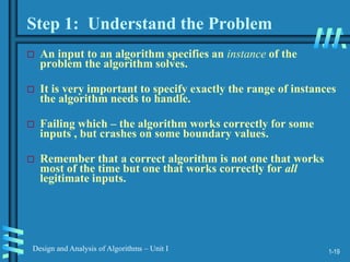
An input to an algorithm specifies an instance of the
problem the algorithm solves.
It is very important to specify exactly the range of instances
the algorithm needs to handle.
Failing which – the algorithm works correctly for some
inputs , but crashes on some boundary values.
Remember that a correct algorithm is not one that works
most of the time but one that works correctly for all
legitimate inputs.
Step 1: Understand the Problem
21.
1-20
Design and Analysisof Algorithms – Unit I
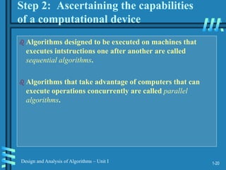
Step 2: Ascertaining the capabilities
of a computational device
Algorithms designed to be executed on machines that
executes intstructions one after another are called
sequential algorithms.
Algorithms that take advantage of computers that can
execute operations concurrently are called parallel
algorithms.
22.
1-21
Design and Analysisof Algorithms – Unit I
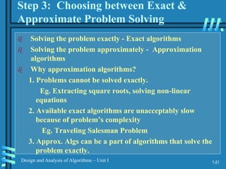
Step 3: Choosing between Exact &
Approximate Problem Solving
Solving the problem exactly - Exact algorithms
Solving the problem approximately - Approximation
algorithms
Why approximation algorithms?
1. Problems cannot be solved exactly.
Eg. Extracting square roots, solving non-linear
equations
2. Available exact algorithms are unacceptably slow
because of problem’s complexity
Eg. Traveling Salesman Problem
3. Approx. Algs can be a part of algorithms that solve the
problem exactly.
23.
1-22
Design and Analysisof Algorithms – Unit I
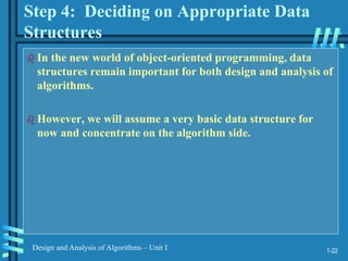
Step 4: Deciding on Appropriate Data
Structures
In the new world of object-oriented programming, data
structures remain important for both design and analysis of
algorithms.
However, we will assume a very basic data structure for
now and concentrate on the algorithm side.
24.
1-23
Design and Analysisof Algorithms – Unit I
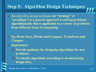
Step 5: Algorithm Design Techniques
An algorithm design technique (or “strategy” or
“paradigm”) is a general approach to solving problems
algorithmically that is applicable to a variety of problems
from different areas of computing.
Eg. Brute force, Divide-and-Conquer, Transform-and-
Conquer
Importance:
1. Provide guidance for designing algorithms for new
problems.
2. To classify algorithms according to an underlying
design idea.
25.
1-24
Design and Analysisof Algorithms – Unit I
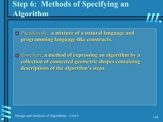
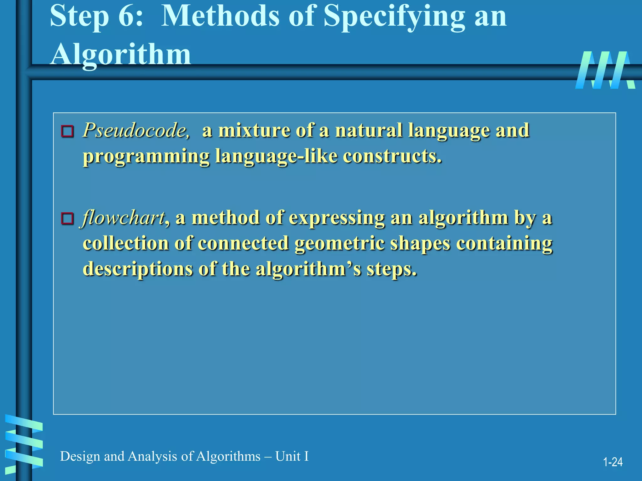
Step 6: Methods of Specifying an
Algorithm
Pseudocode, a mixture of a natural language and
programming language-like constructs.
flowchart, a method of expressing an algorithm by a
collection of connected geometric shapes containing
descriptions of the algorithm’s steps.
26.
1-25
Design and Analysisof Algorithms – Unit I
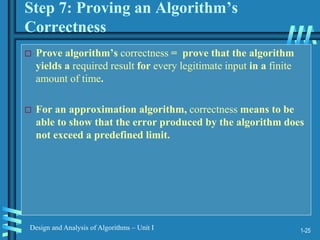
Step 7: Proving an Algorithm’s
Correctness
Prove algorithm’s correctness = prove that the algorithm
yields a required result for every legitimate input in a finite
amount of time.
For an approximation algorithm, correctness means to be
able to show that the error produced by the algorithm does
not exceed a predefined limit.
27.
1-26
Design and Analysisof Algorithms – Unit I
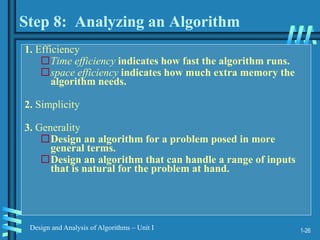
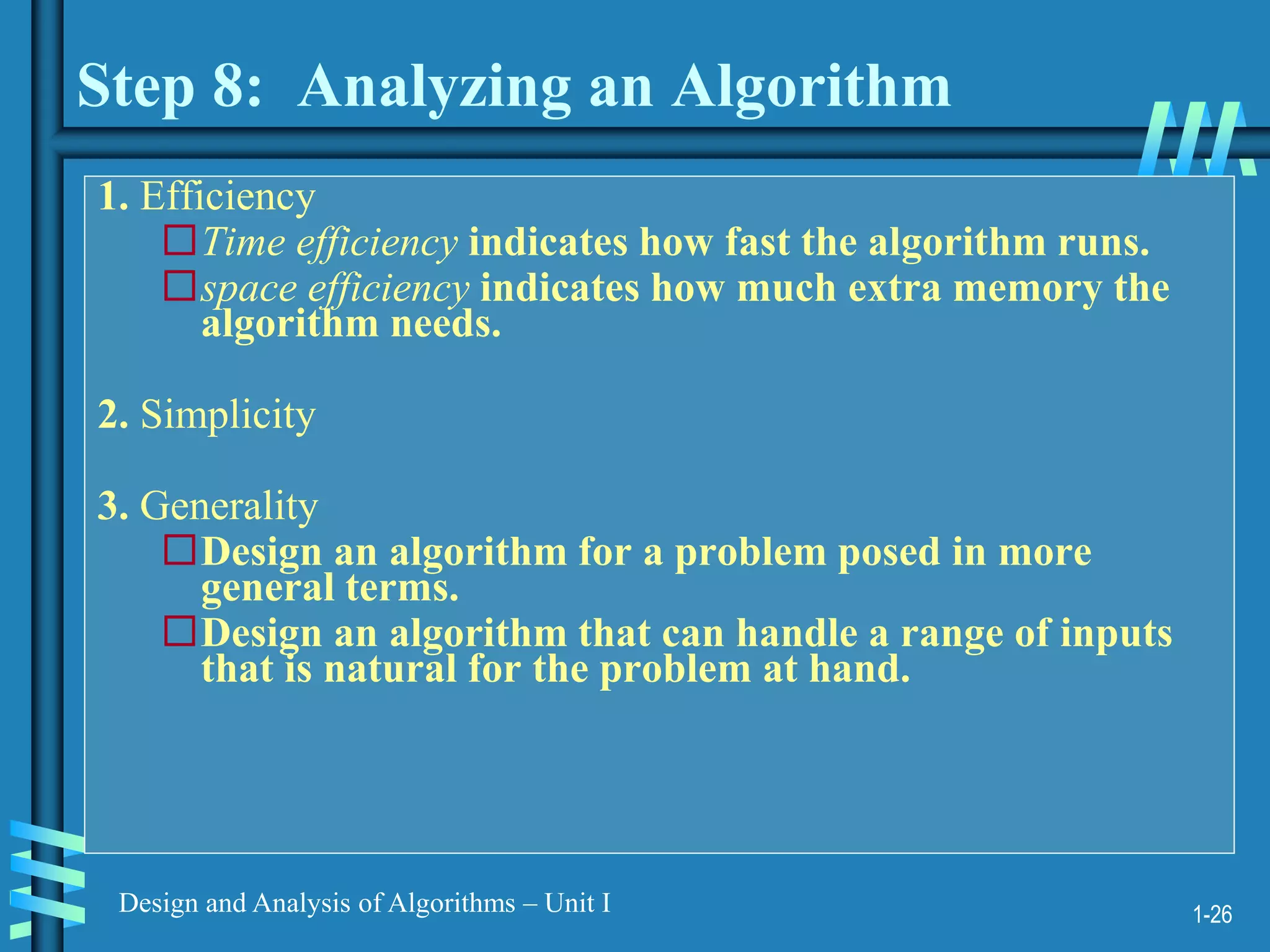
Step 8: Analyzing an Algorithm
1. Efficiency
Time efficiency indicates how fast the algorithm runs.
space efficiency indicates how much extra memory the
algorithm needs.
2. Simplicity
3. Generality
Design an algorithm for a problem posed in more
general terms.
Design an algorithm that can handle a range of inputs
that is natural for the problem at hand.
28.
1-27
Design and Analysisof Algorithms – Unit I
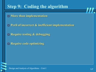
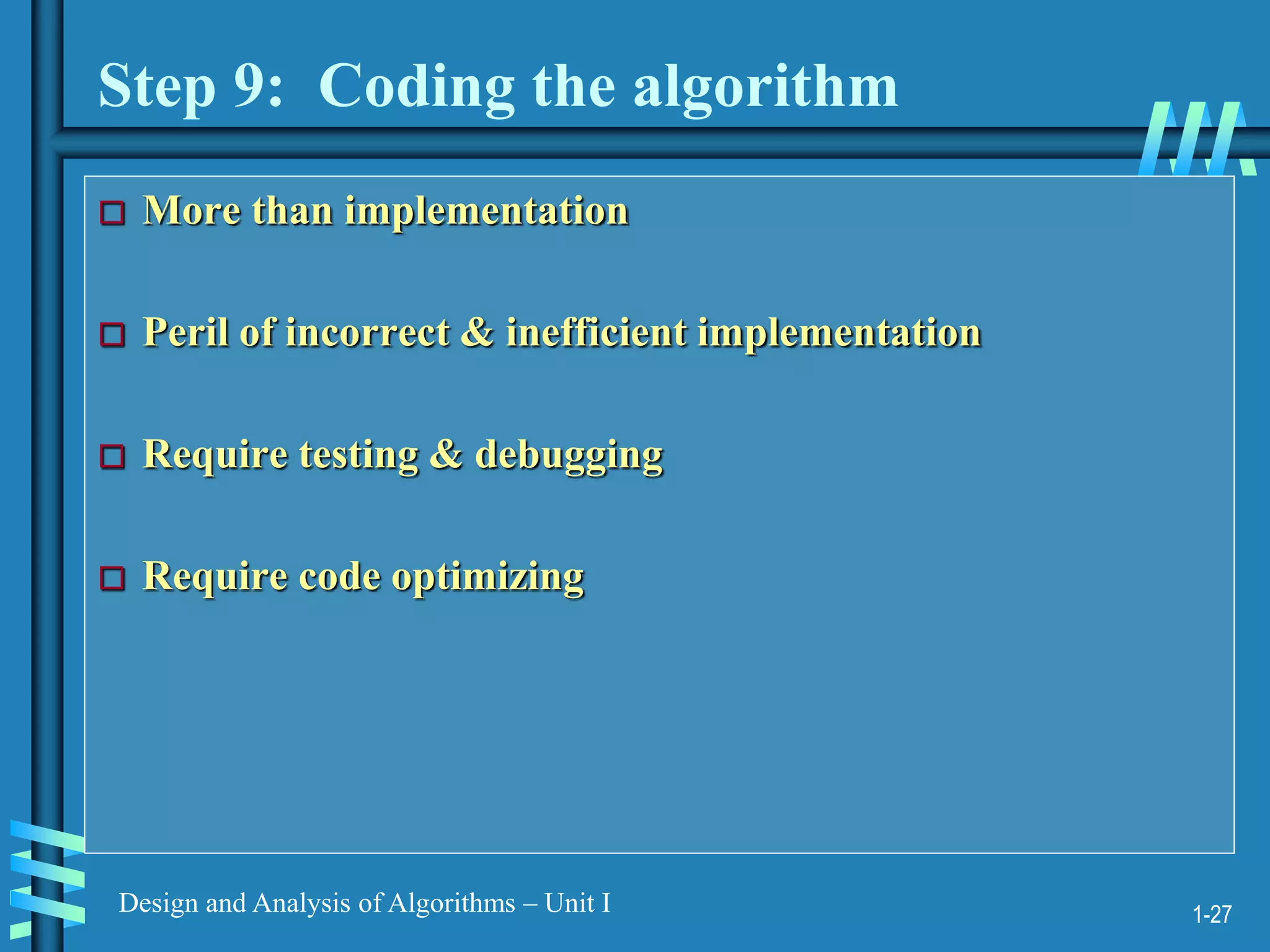
Step 9: Coding the algorithm
More than implementation
Peril of incorrect & inefficient implementation
Require testing & debugging
Require code optimizing
1-29
Design and Analysisof Algorithms – Unit I
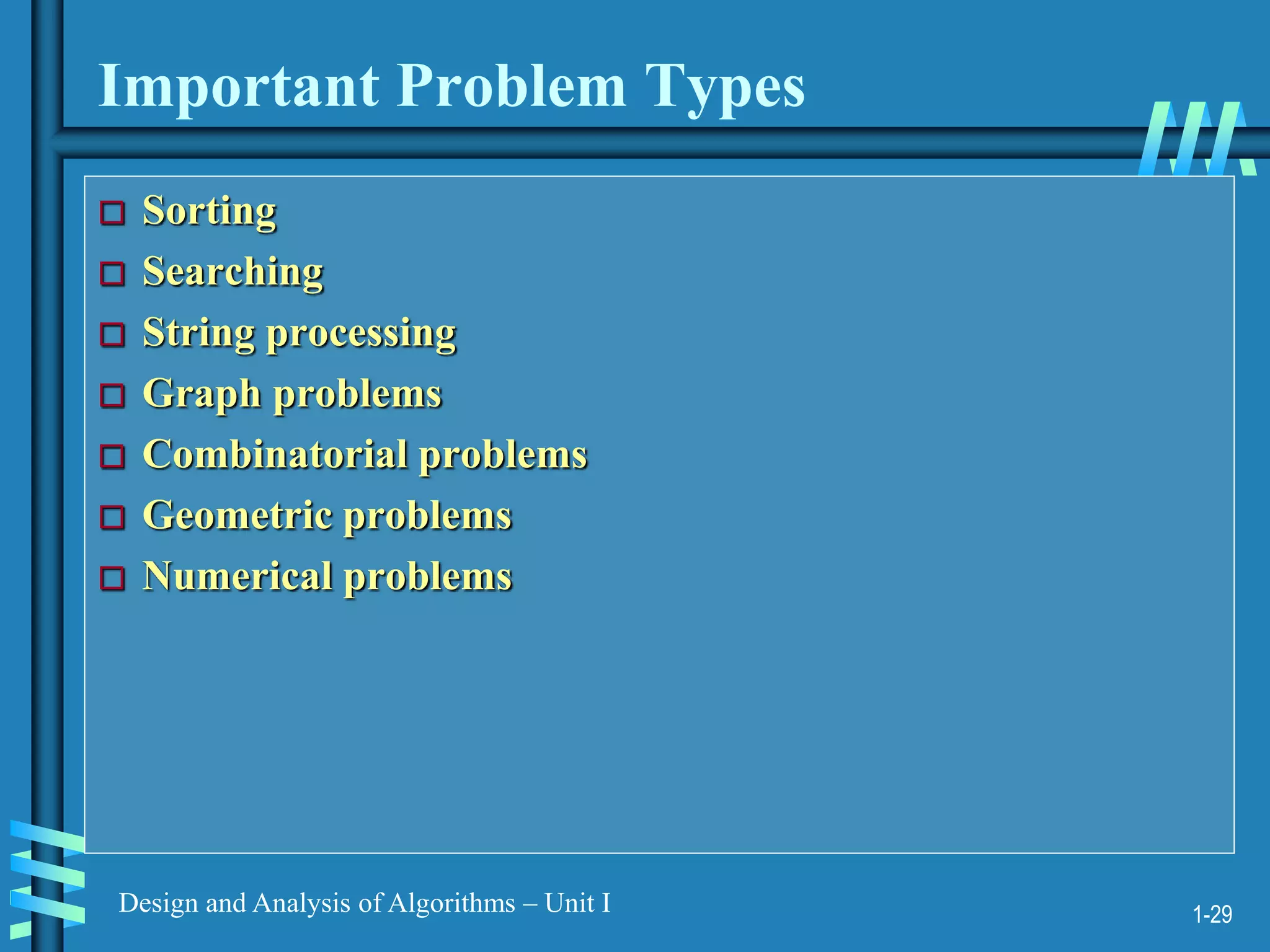
Important Problem Types
Sorting
Searching
String processing
Graph problems
Combinatorial problems
Geometric problems
Numerical problems
31.
1-30
Design and Analysisof Algorithms – Unit I
Sorting
The sorting problem asks us to rearrange the items of a
given list in ascending order.
we usually need to
sort lists of numbers,
characters from an alphabet,
character strings,
records similar to those maintained by schools about
their students,
libraries about their holdings,
companies about their employees.
32.
1-31
Design and Analysisof Algorithms – Unit I
Searching
The searching problem deals with finding a given value,
called a search key, in a given set (or a multiset, which
permits several elements to have the same value).
33.
1-32
Design and Analysisof Algorithms – Unit I
String Processing
A string is a sequence of characters from an alphabet.
String of particular interest:
1. Text string – comprises letters, numbers, and special
characters
2. Bit string – comprises zeros and ones
3. Gene sequence
Mainly string matching problem: searching for a given
word in a text
34.
1-33
Design and Analysisof Algorithms – Unit I
Graph Problems
A graph can be thought of as a collection of points called
vertices, some of which are connected by line segments
called edges.
Used for modeling a wide variety of real-life applications.
Basic graph algorithms include:
1. Graph traversal algorithms - How can one visit all the
points in a network?
2. Shortest-path algorithms - What is the best Introduction
route between two cities?
3. Topological sorting for graphs with directed edges
35.
1-34
Design and Analysisof Algorithms – Unit I
Combinatorial Problems
combinatorial problems: problems that ask (explicitly or
implicitly) to find a combinatorial object—such as a
permutation, a combination, or a subset—that satisfies
certain constraints and has some desired property (e.g.,
maximizes a value or minimizes a cost).
1. Combinatorial grows extremely fast with problem size
2. No known algorithm solving most such problems
exactly in an acceptable amount of time.
36.
1-35
Design and Analysisof Algorithms – Unit I
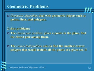
Geometric Problems
Geometric algorithms deal with geometric objects such as
points, lines, and polygons.
2 class problems:
The closest pair problem: given n points in the plane, find
the closest pair among them.
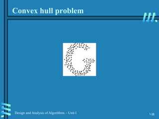
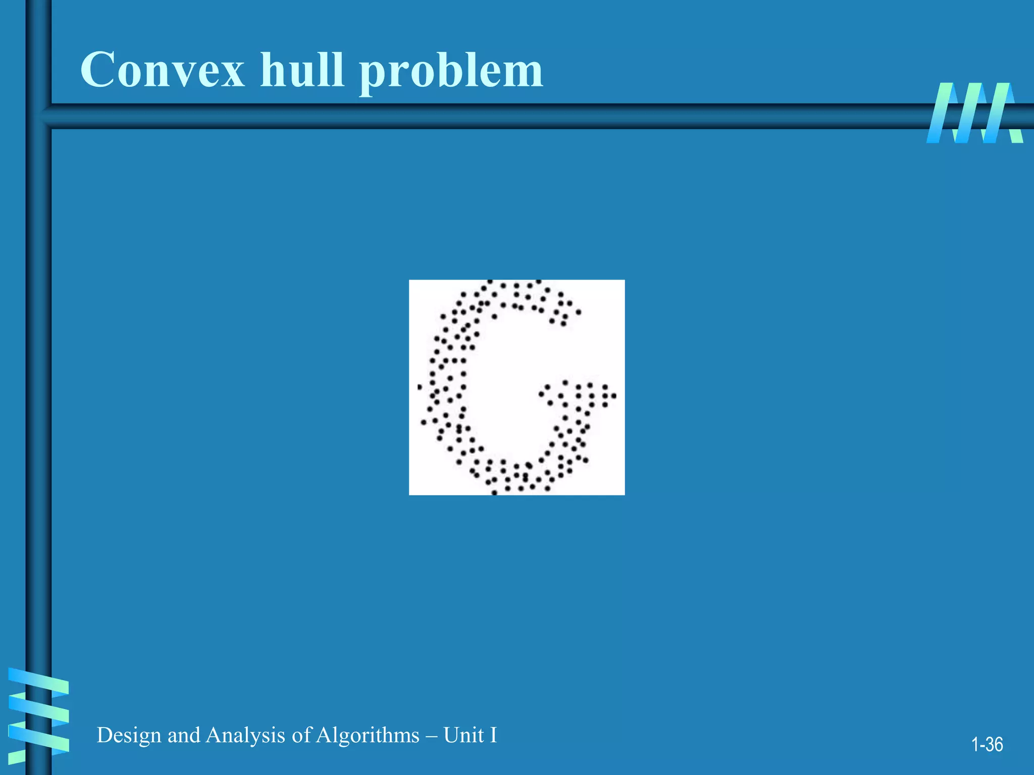
The convex hull problem asks to find the smallest convex
polygon that would include all the points of a given set. If
1-37
Design and Analysisof Algorithms – Unit I
Numerical Problems
Numerical problems, another large special area of
applications, are problems that involve mathematical
objects of continuous nature: solving equations and systems
of equations, computing definite integrals, evaluating
functions, and so on.
1-39
Design and Analysisof Algorithms – Unit I
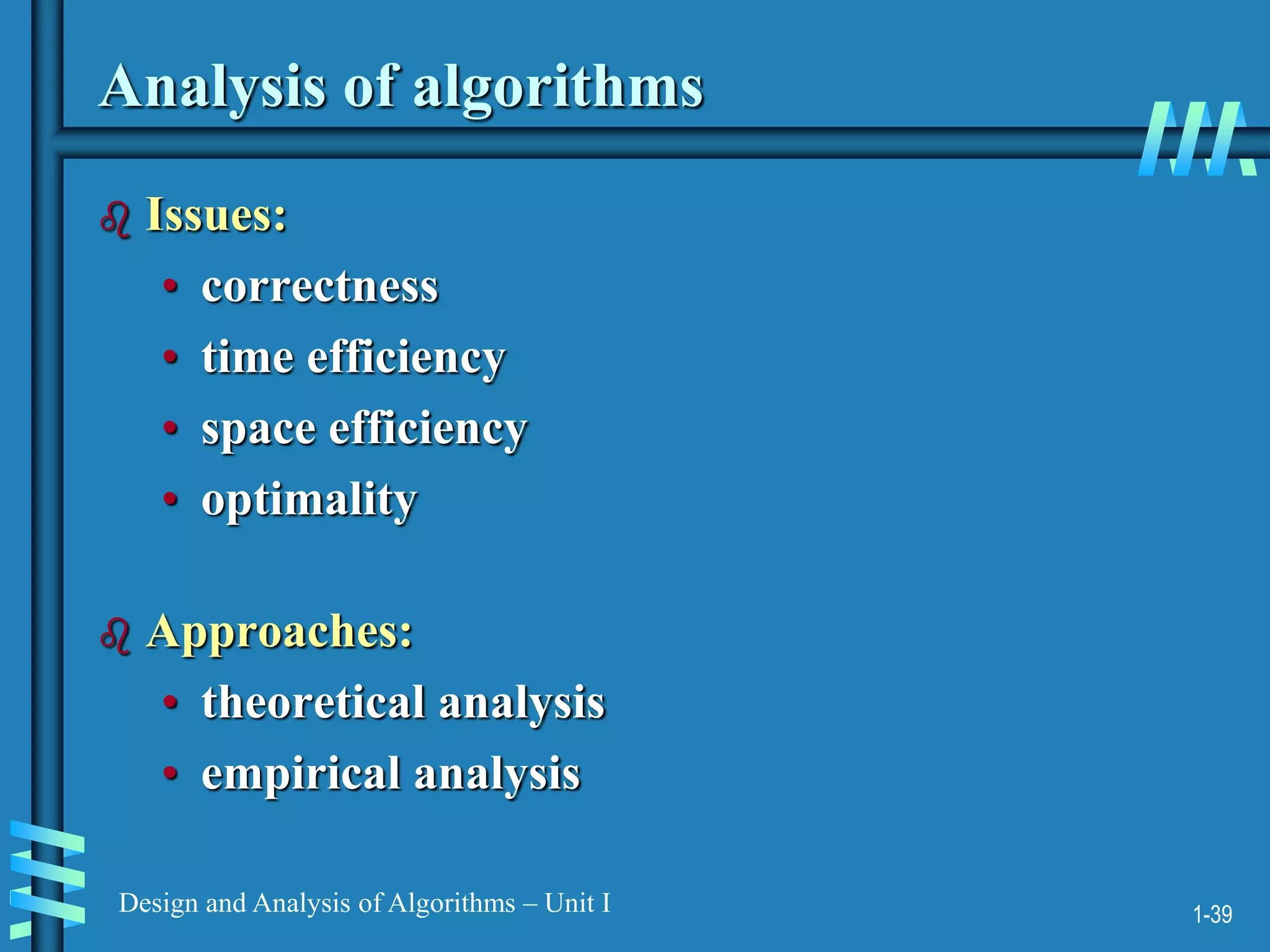
Analysis of algorithms
Issues:
• correctness
• time efficiency
• space efficiency
• optimality
Approaches:
• theoretical analysis
• empirical analysis
41.
1-40
Design and Analysisof Algorithms – Unit I
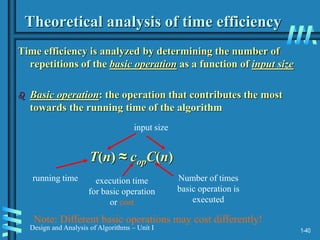
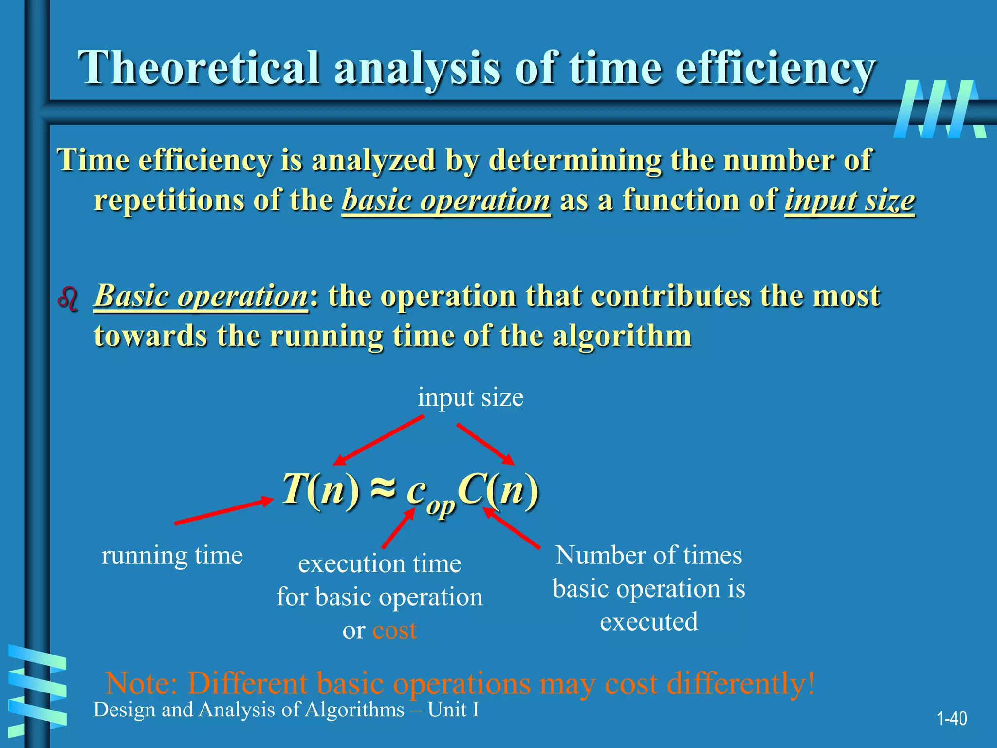
Theoretical analysis of time efficiency
Time efficiency is analyzed by determining the number of
repetitions of the basic operation as a function of input size
Basic operation: the operation that contributes the most
towards the running time of the algorithm
T(n) ≈ copC(n)
running time execution time
for basic operation
or cost
Number of times
basic operation is
executed
input size
Note: Different basic operations may cost differently!
42.
1-41
Design and Analysisof Algorithms – Unit I
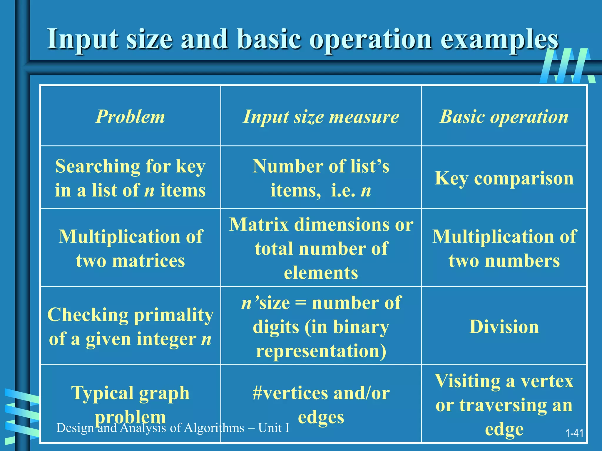
Input size and basic operation examples
Problem Input size measure Basic operation
Searching for key
in a list of n items
Number of list’s
items, i.e. n
Key comparison
Multiplication of
two matrices
Matrix dimensions or
total number of
elements
Multiplication of
two numbers
Checking primality
of a given integer n
n’size = number of
digits (in binary
representation)
Division
Typical graph
problem
#vertices and/or
edges
Visiting a vertex
or traversing an
edge
43.
1-42
Design and Analysisof Algorithms – Unit I
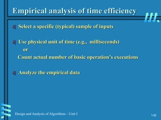
Empirical analysis of time efficiency
Select a specific (typical) sample of inputs
Use physical unit of time (e.g., milliseconds)
or
Count actual number of basic operation’s executions
Analyze the empirical data
44.
1-43
Design and Analysisof Algorithms – Unit I
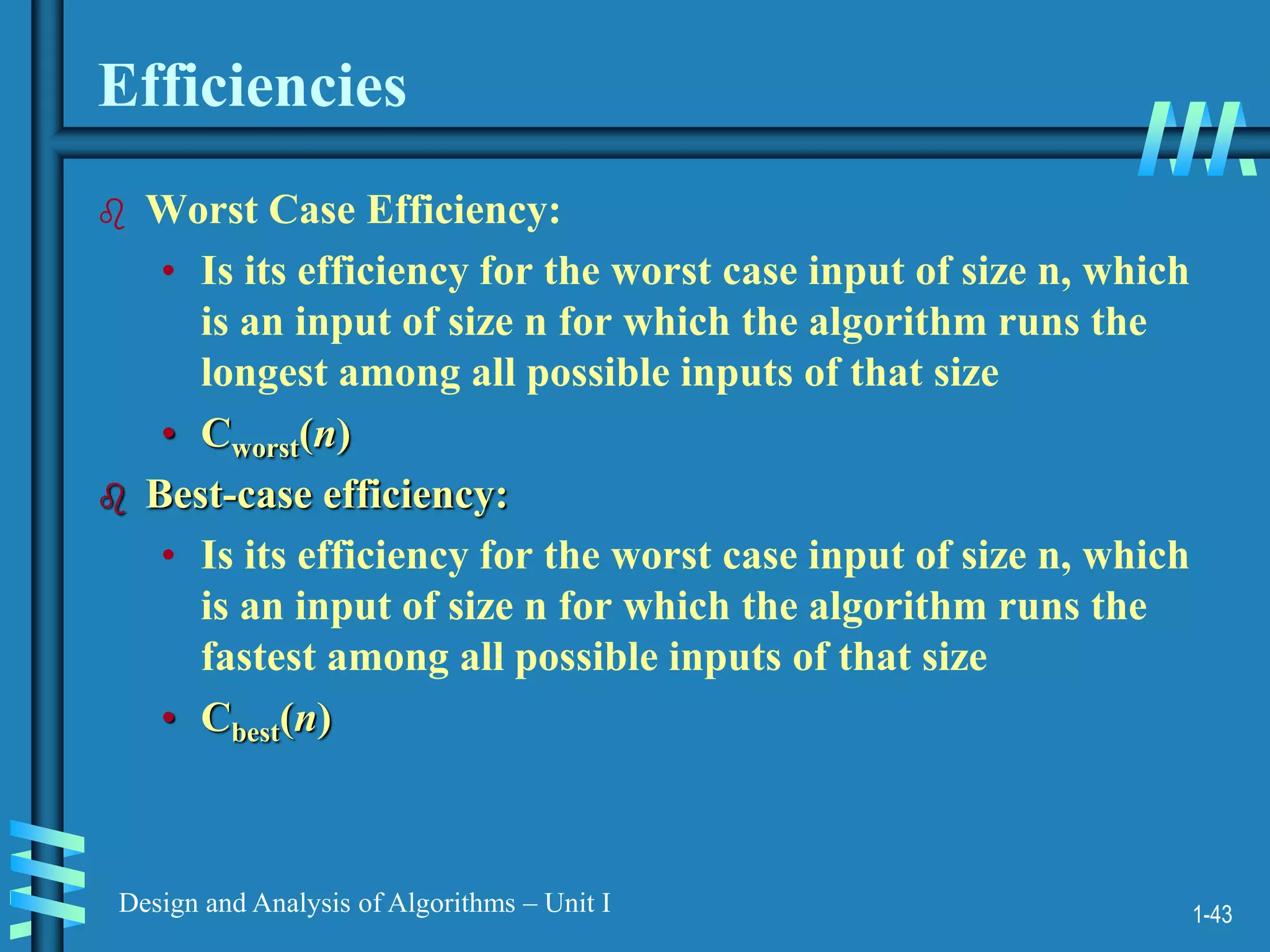
Efficiencies
Worst Case Efficiency:
• Is its efficiency for the worst case input of size n, which
is an input of size n for which the algorithm runs the
longest among all possible inputs of that size
• Cworst(n)
Best-case efficiency:
• Is its efficiency for the worst case input of size n, which
is an input of size n for which the algorithm runs the
fastest among all possible inputs of that size
• Cbest(n)
45.
1-44
Design and Analysisof Algorithms – Unit I
Amortized efficiency
• It applies not to a single run of an
algorithm, but rather to a sequence of
operations performed on the same data
structure
46.
1-45
Design and Analysisof Algorithms – Unit I
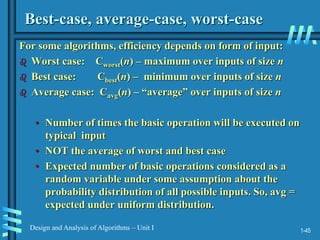
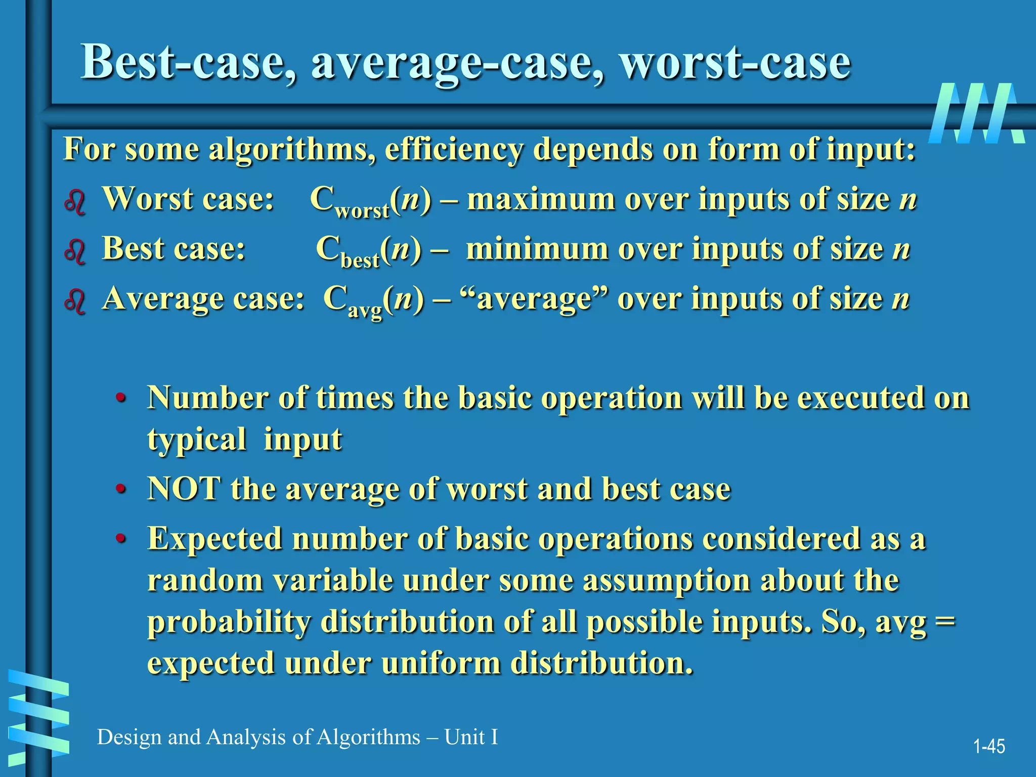
Best-case, average-case, worst-case
For some algorithms, efficiency depends on form of input:
Worst case: Cworst(n) – maximum over inputs of size n
Best case: Cbest(n) – minimum over inputs of size n
Average case: Cavg(n) – “average” over inputs of size n
• Number of times the basic operation will be executed on
typical input
• NOT the average of worst and best case
• Expected number of basic operations considered as a
random variable under some assumption about the
probability distribution of all possible inputs. So, avg =
expected under uniform distribution.
47.
1-46
Design and Analysisof Algorithms – Unit I
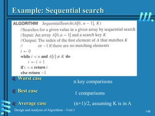
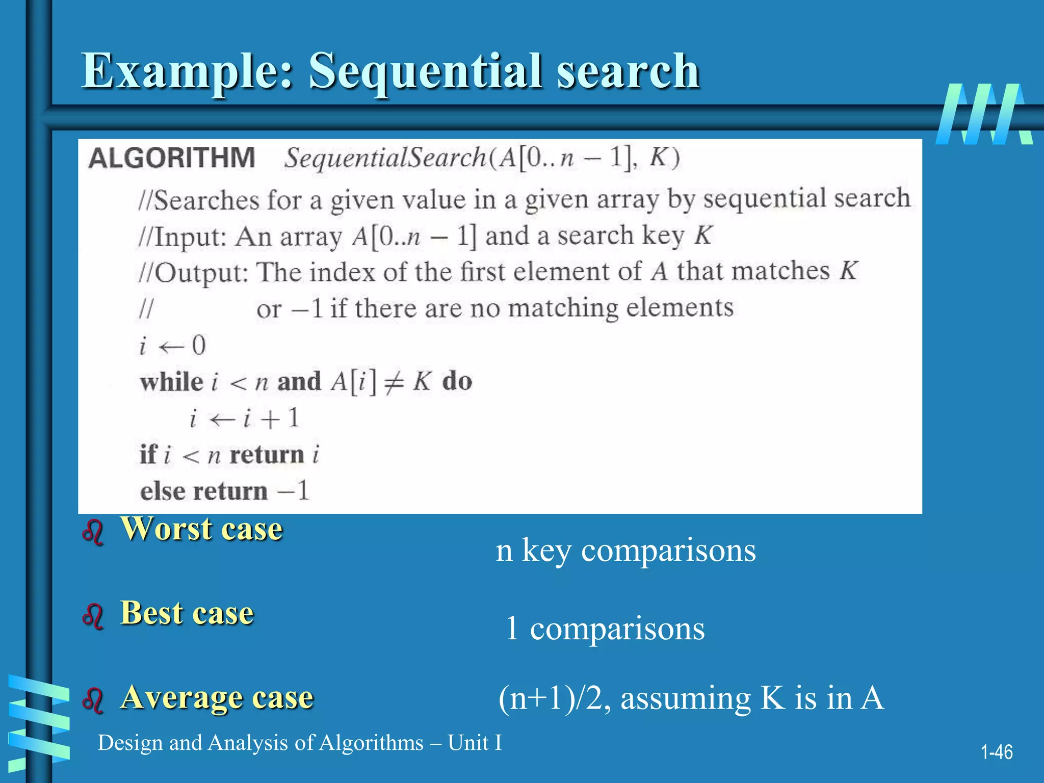
Example: Sequential search
Worst case
Best case
Average case
n key comparisons
1 comparisons
(n+1)/2, assuming K is in A
48.
1-47
Design and Analysisof Algorithms – Unit I
Types of formulas for basic operation’s count
Exact formula
e.g., C(n) = n(n-1)/2
Formula indicating order of growth with specific
multiplicative constant
e.g., C(n) ≈ 0.5 n2
Formula indicating order of growth with unknown
multiplicative constant
e.g., C(n) ≈ cn2
49.
1-48
Design and Analysisof Algorithms – Unit I
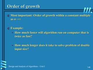
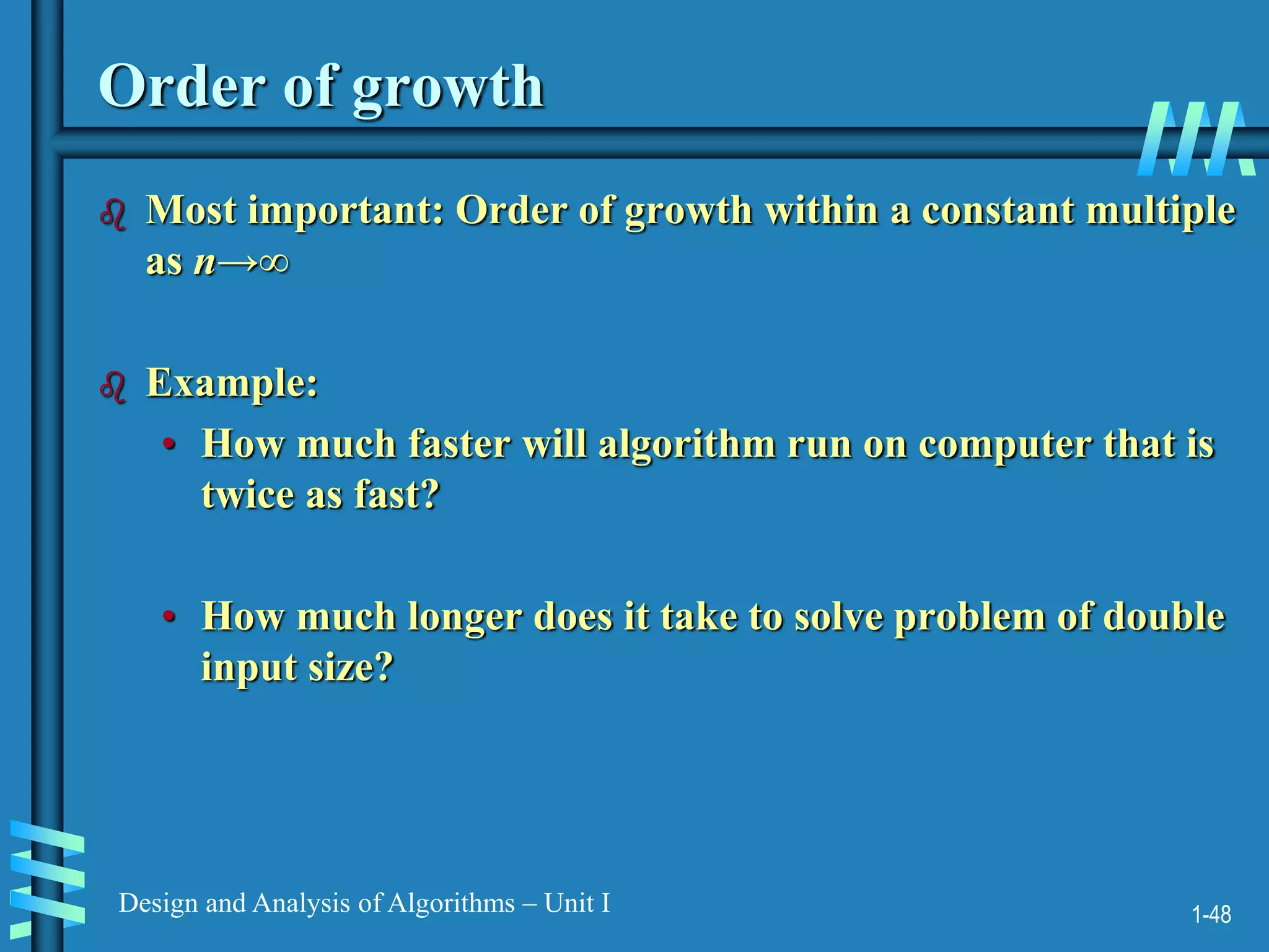
Order of growth
Most important: Order of growth within a constant multiple
as n→∞
Example:
• How much faster will algorithm run on computer that is
twice as fast?
• How much longer does it take to solve problem of double
input size?
1-50
Design and Analysisof Algorithms – Unit I
Asymptotic Notations
O (Big-Oh)-notation
Ω (Big-Omega) -notation
Θ (Big-Theta) -notation
52.
1-51
Design and Analysisof Algorithms – Unit I
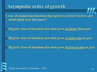
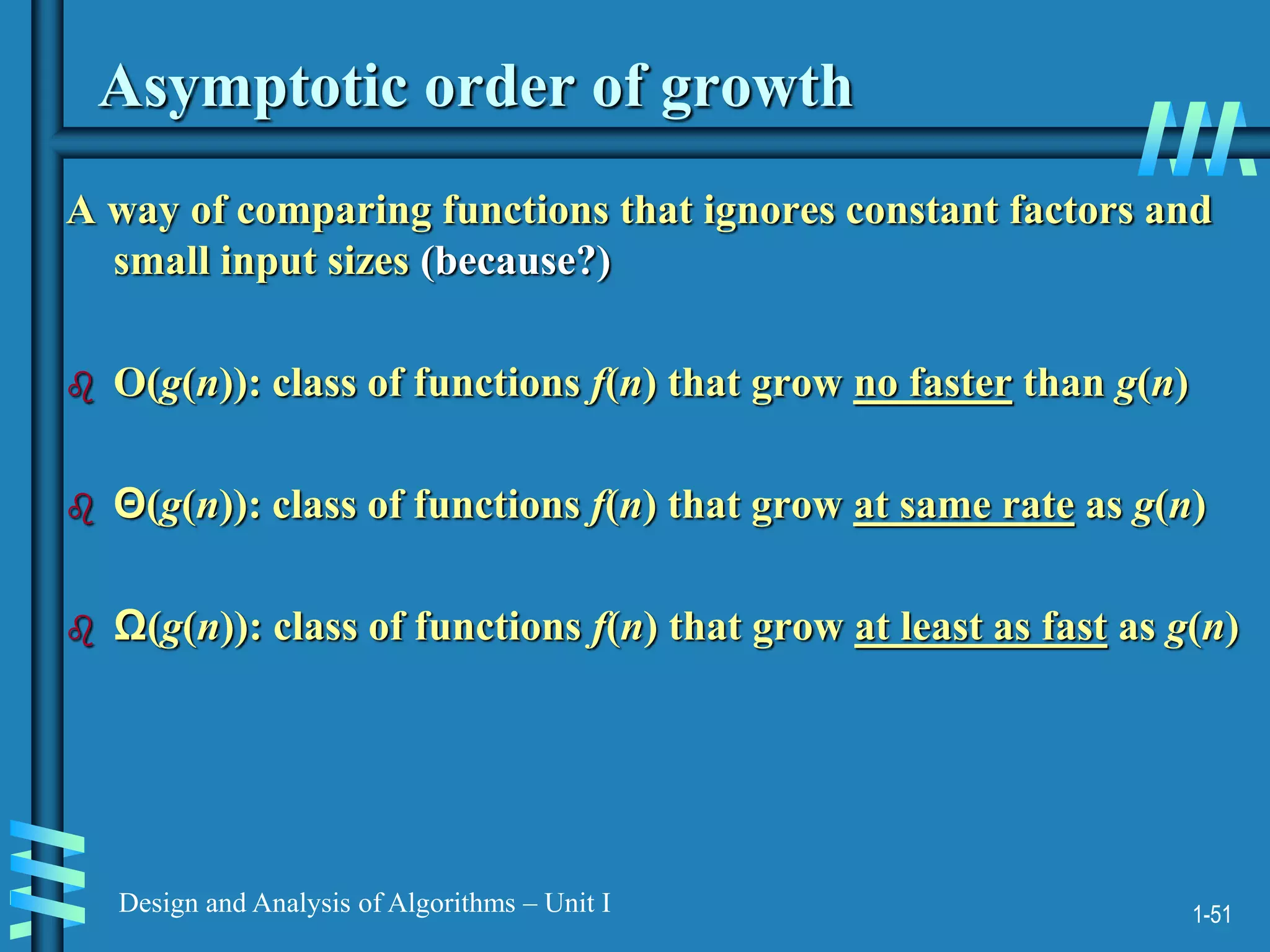
Asymptotic order of growth
A way of comparing functions that ignores constant factors and
small input sizes (because?)
O(g(n)): class of functions f(n) that grow no faster than g(n)
Θ(g(n)): class of functions f(n) that grow at same rate as g(n)
Ω(g(n)): class of functions f(n) that grow at least as fast as g(n)
53.
1-52
Design and Analysisof Algorithms – Unit I
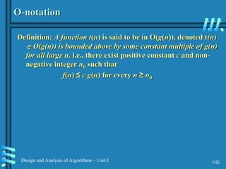
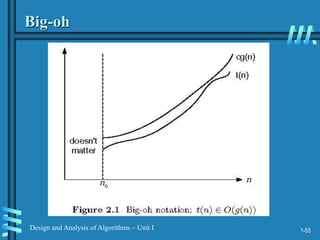
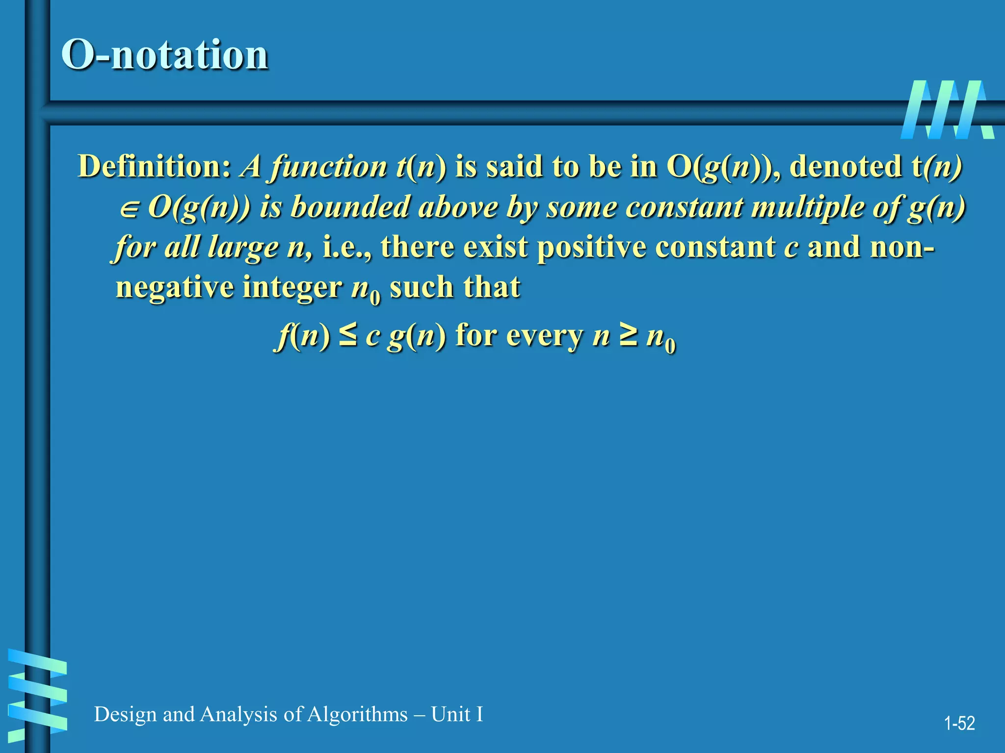
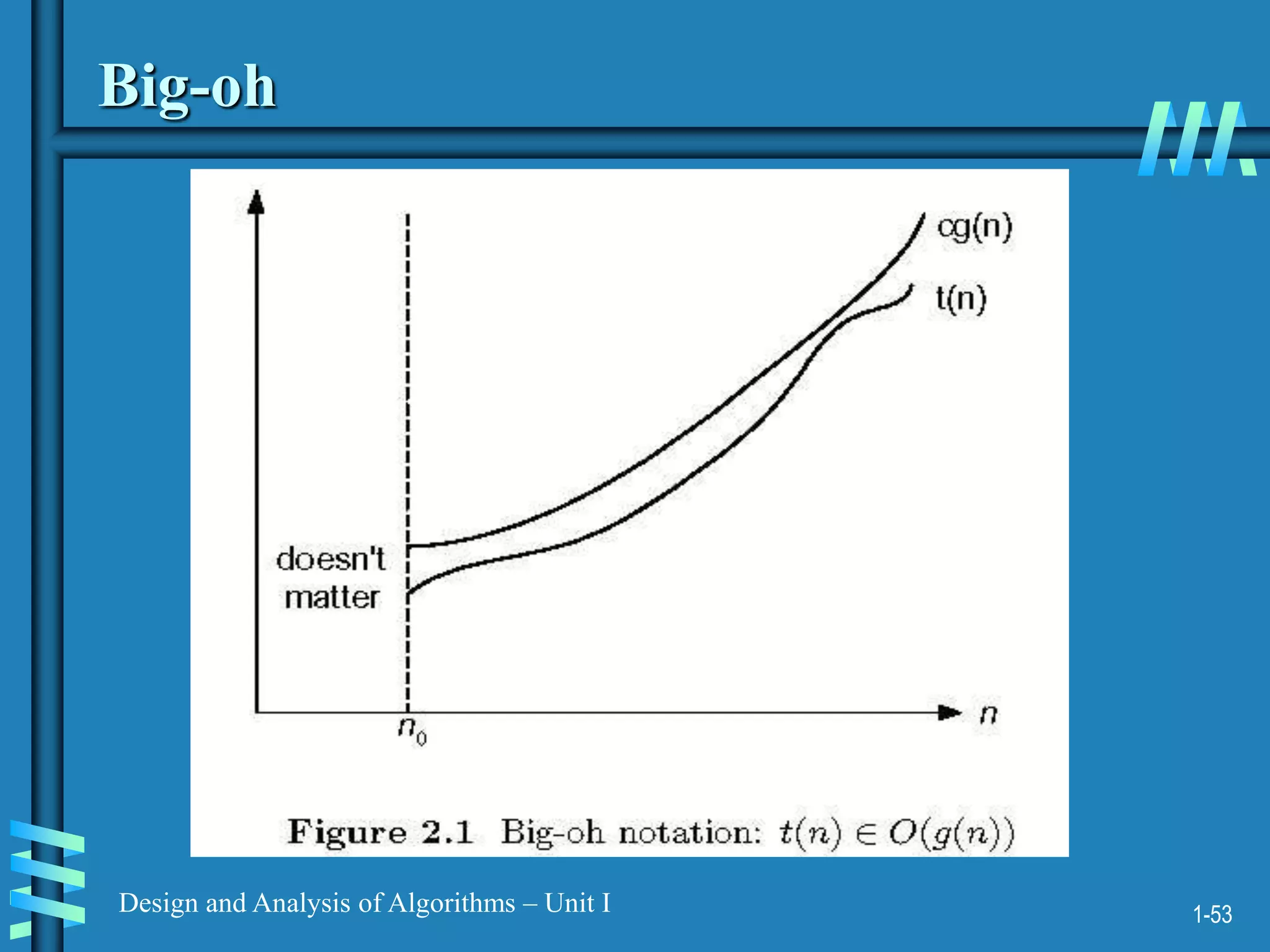
O-notation
Definition: A function t(n) is said to be in O(g(n)), denoted t(n)
O(g(n)) is bounded above by some constant multiple of g(n)
for all large n, i.e., there exist positive constant c and non-
negative integer n0 such that
f(n) ≤ c g(n) for every n ≥ n0
1-54
Design and Analysisof Algorithms – Unit I
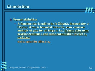
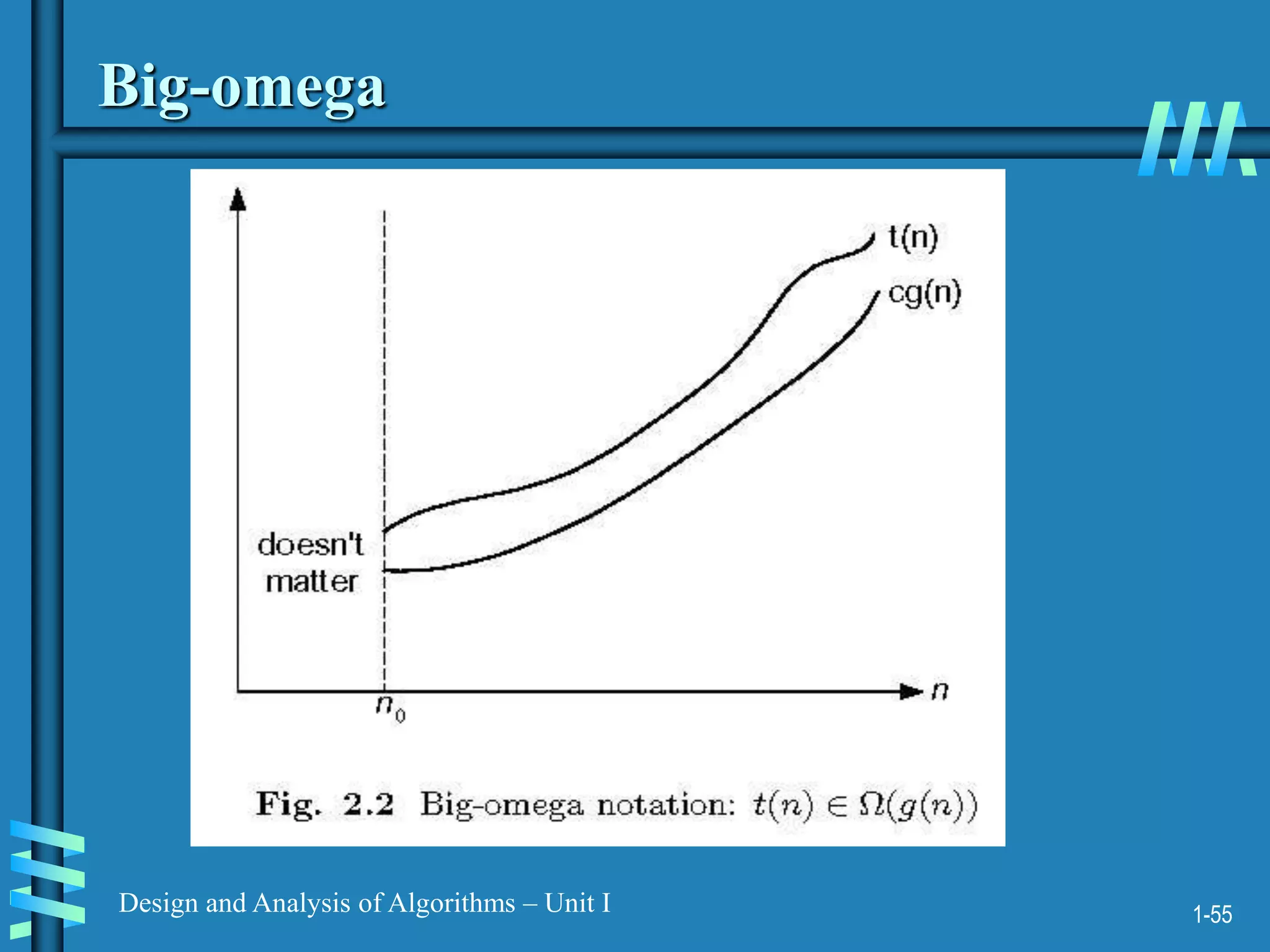
-notation
Formal definition
• A function t(n) is said to be in (g(n)), denoted t(n)
(g(n)), if t(n) is bounded below by some constant
multiple of g(n) for all large n, i.e., if there exist some
positive constant c and some nonnegative integer n0
such that
t(n) cg(n) for all n n0
1-56
Design and Analysisof Algorithms – Unit I
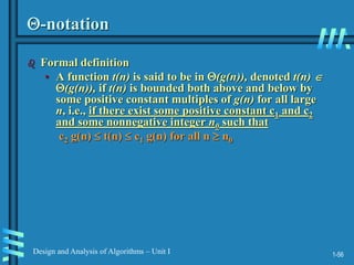
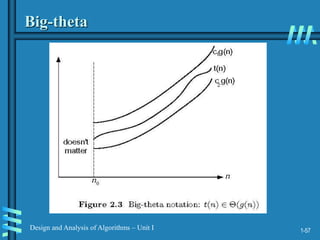
-notation
Formal definition
• A function t(n) is said to be in (g(n)), denoted t(n)
(g(n)), if t(n) is bounded both above and below by
some positive constant multiples of g(n) for all large
n, i.e., if there exist some positive constant c1 and c2
and some nonnegative integer n0 such that
c2 g(n) t(n) c1 g(n) for all n n0
1-58
Design and Analysisof Algorithms – Unit I
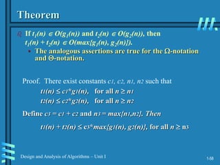
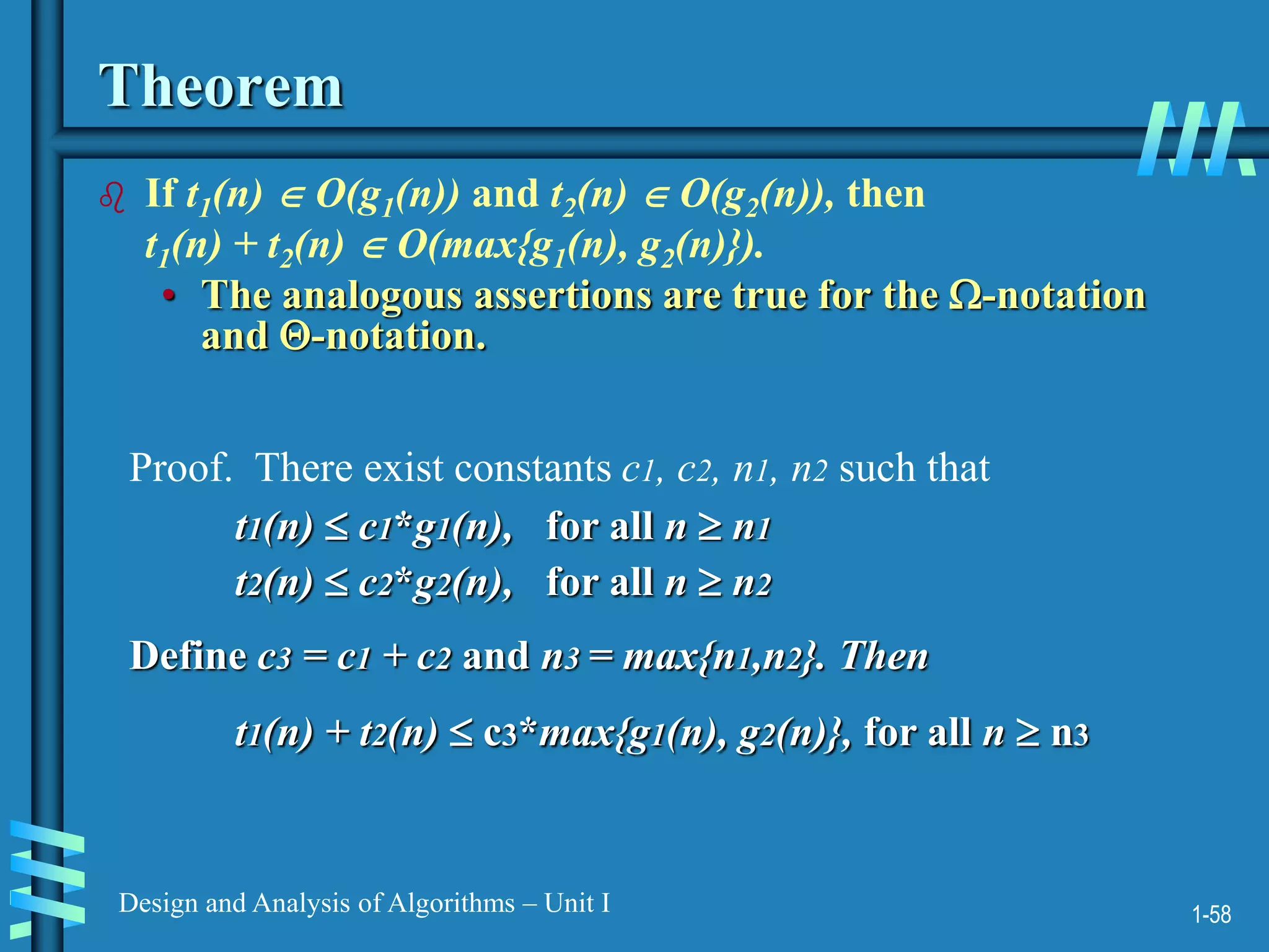
Theorem
If t1(n) O(g1(n)) and t2(n) O(g2(n)), then
t1(n) + t2(n) O(max{g1(n), g2(n)}).
• The analogous assertions are true for the -notation
and -notation.
Proof. There exist constants c1, c2, n1, n2 such that
t1(n) c1*g1(n), for all n n1
t2(n) c2*g2(n), for all n n2
Define c3 = c1 + c2 and n3 = max{n1,n2}. Then
t1(n) + t2(n) c3*max{g1(n), g2(n)}, for all n n3
60.
1-59
Design and Analysisof Algorithms – Unit I
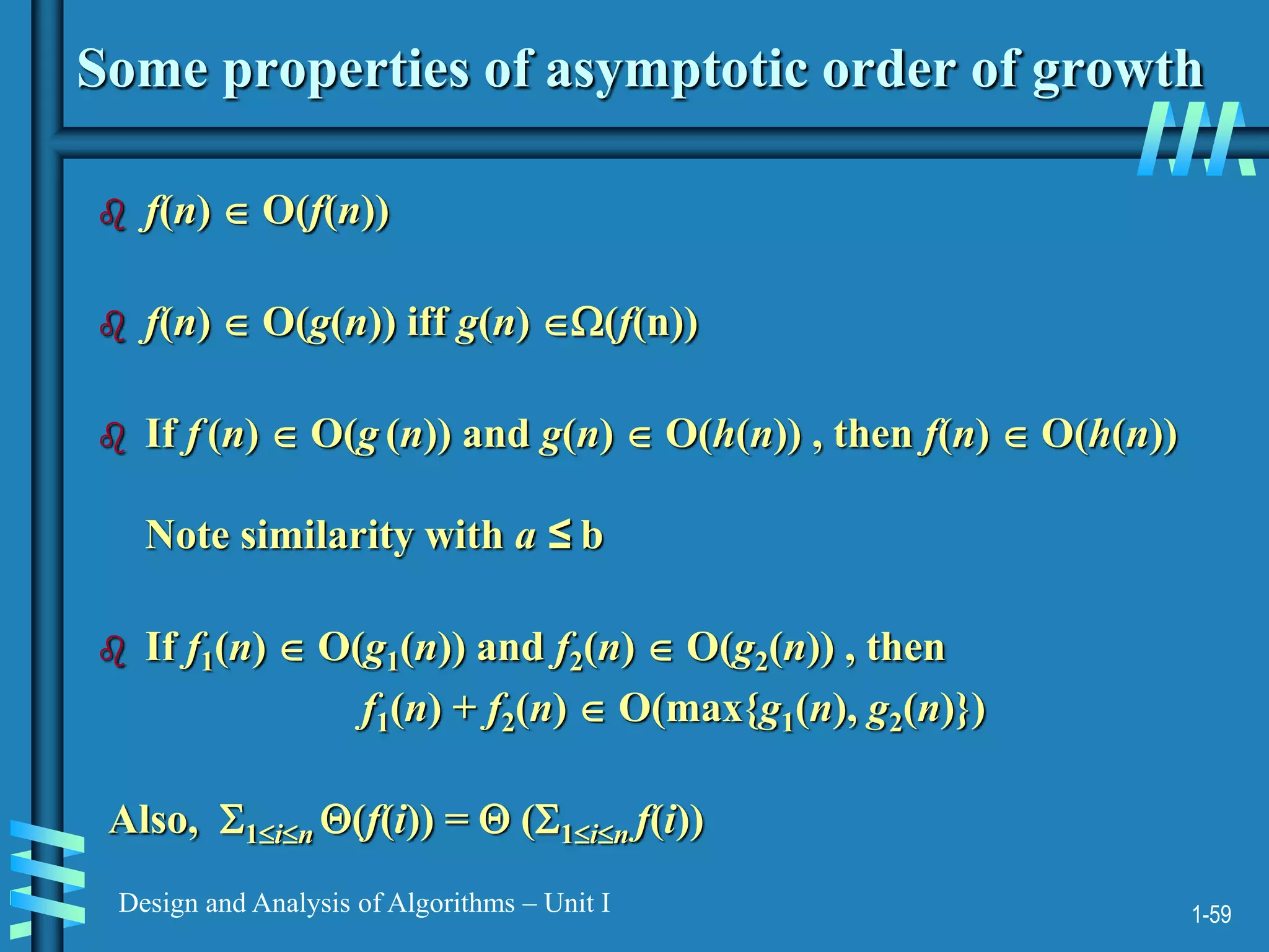
Some properties of asymptotic order of growth
f(n) O(f(n))
f(n) O(g(n)) iff g(n) (f(n))
If f (n) O(g (n)) and g(n) O(h(n)) , then f(n) O(h(n))
Note similarity with a ≤ b
If f1(n) O(g1(n)) and f2(n) O(g2(n)) , then
f1(n) + f2(n) O(max{g1(n), g2(n)})
Also, 1in (f(i)) = (1in f(i))
61.
1-60
Design and Analysisof Algorithms – Unit I
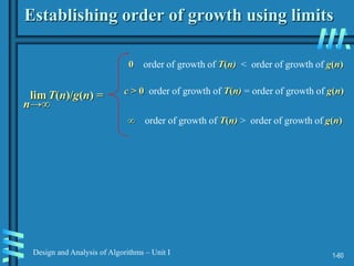
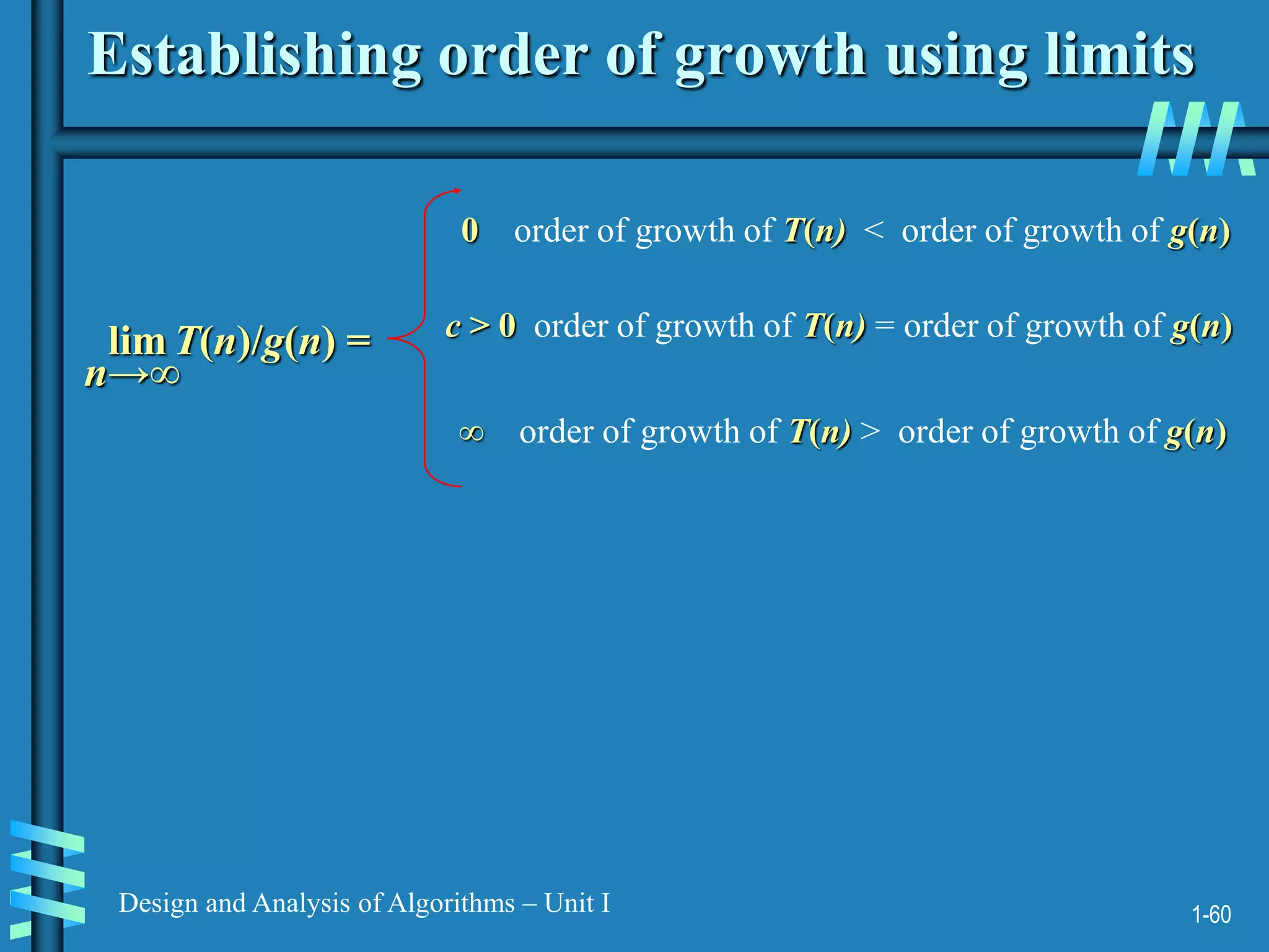
Establishing order of growth using limits
lim T(n)/g(n) =
0 order of growth of T(n) < order of growth of g(n)
c > 0 order of growth of T(n) = order of growth of g(n)
∞ order of growth of T(n) > order of growth of g(n)
n→∞
62.
1-61
Design and Analysisof Algorithms – Unit I
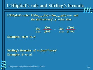
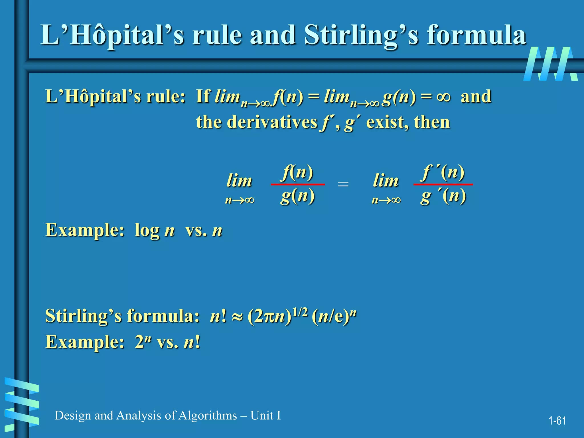
L’Hôpital’s rule and Stirling’s formula
L’Hôpital’s rule: If limn f(n) = limn g(n) = and
the derivatives f´, g´ exist, then
Stirling’s formula: n! (2n)1/2 (n/e)n
f(n)
g(n)
lim
n
=
f ´(n)
g ´(n)
lim
n
Example: log n vs. n
Example: 2n vs. n!
63.
1-62
Design and Analysisof Algorithms – Unit I
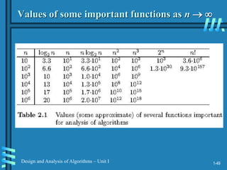
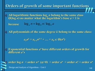
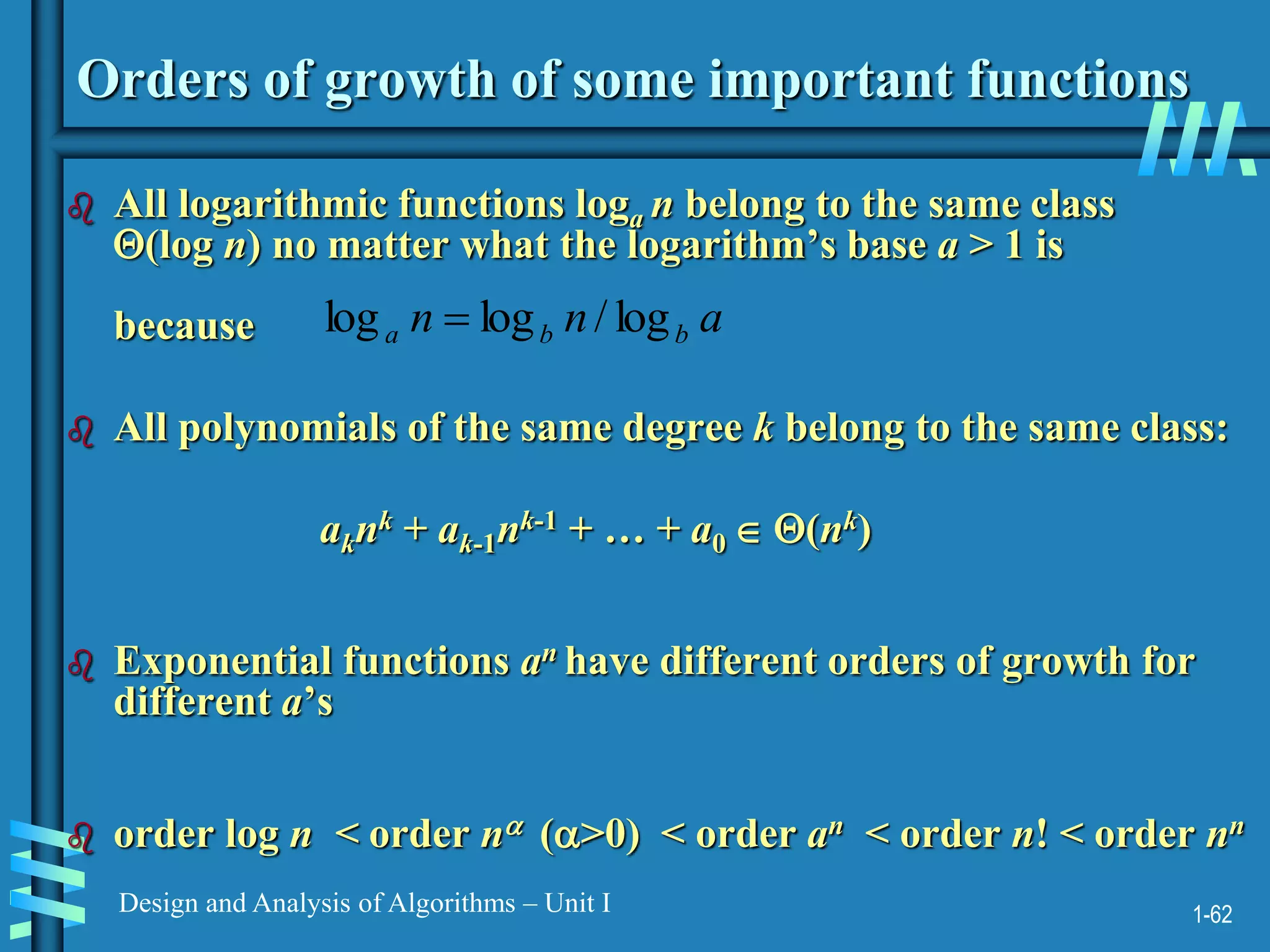
Orders of growth of some important functions
All logarithmic functions loga n belong to the same class
(log n) no matter what the logarithm’s base a > 1 is
because
All polynomials of the same degree k belong to the same class:
aknk + ak-1nk-1 + … + a0 (nk)
Exponential functions an have different orders of growth for
different a’s
order log n < order n (>0) < order an < order n! < order nn
a
n
n b
b
a log
/
log
log
64.
1-63
Design and Analysisof Algorithms – Unit I
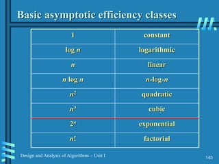
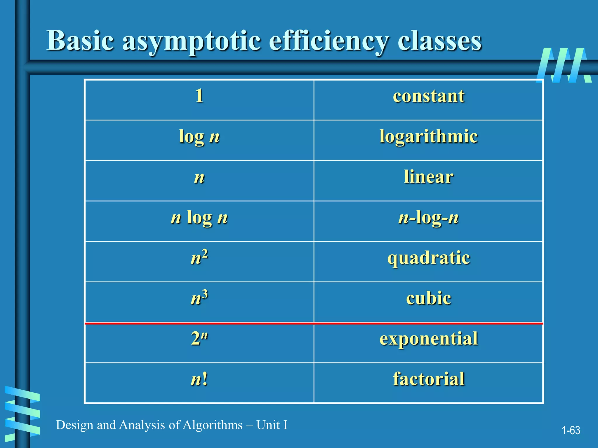
Basic asymptotic efficiency classes
1 constant
log n logarithmic
n linear
n log n n-log-n
n2 quadratic
n3 cubic
2n exponential
n! factorial
65.
1-64
Design and Analysisof Algorithms – Unit I
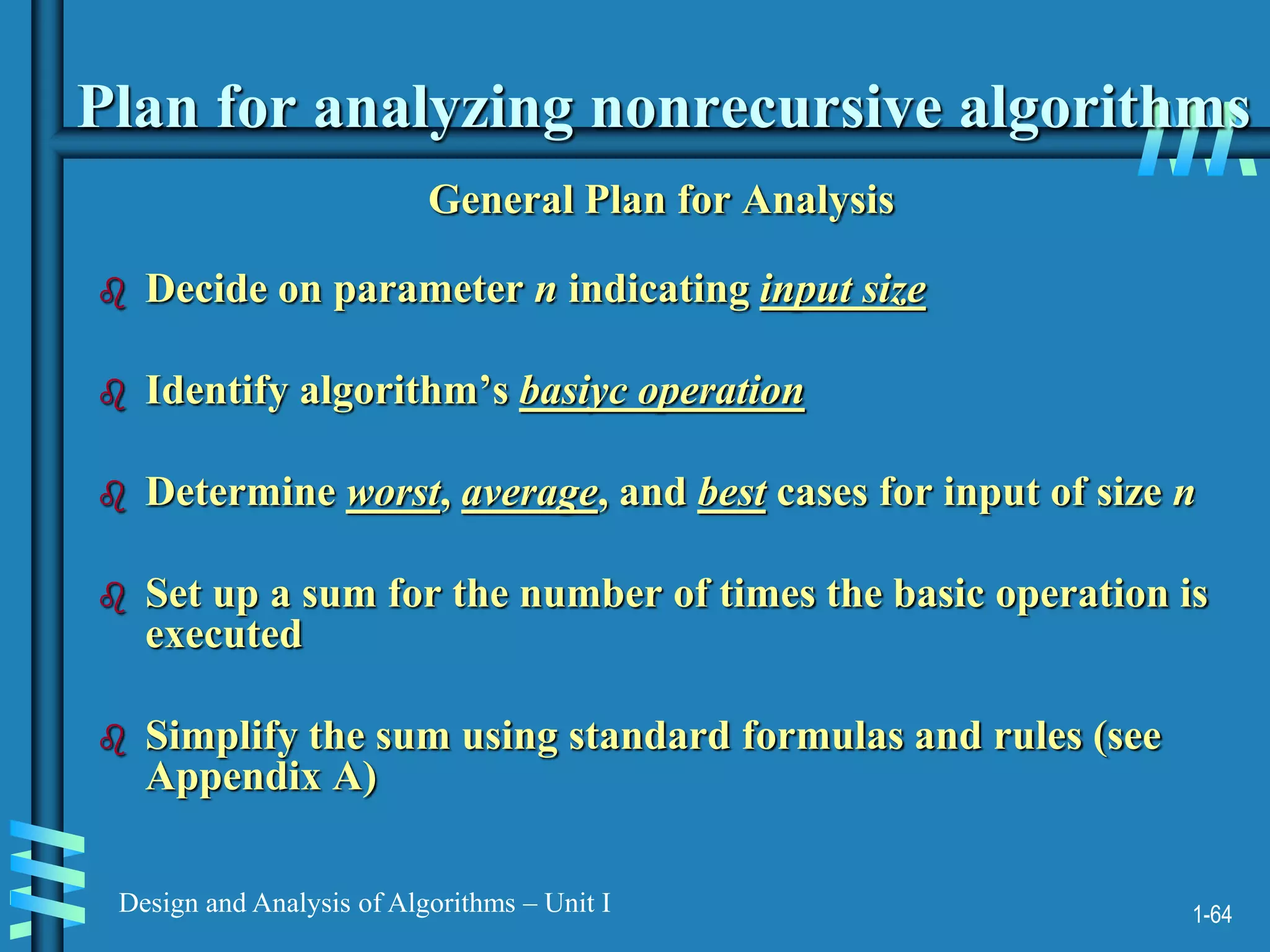
Plan for analyzing nonrecursive algorithms
General Plan for Analysis
Decide on parameter n indicating input size
Identify algorithm’s basiyc operation
Determine worst, average, and best cases for input of size n
Set up a sum for the number of times the basic operation is
executed
Simplify the sum using standard formulas and rules (see
Appendix A)
66.
1-65
Design and Analysisof Algorithms – Unit I
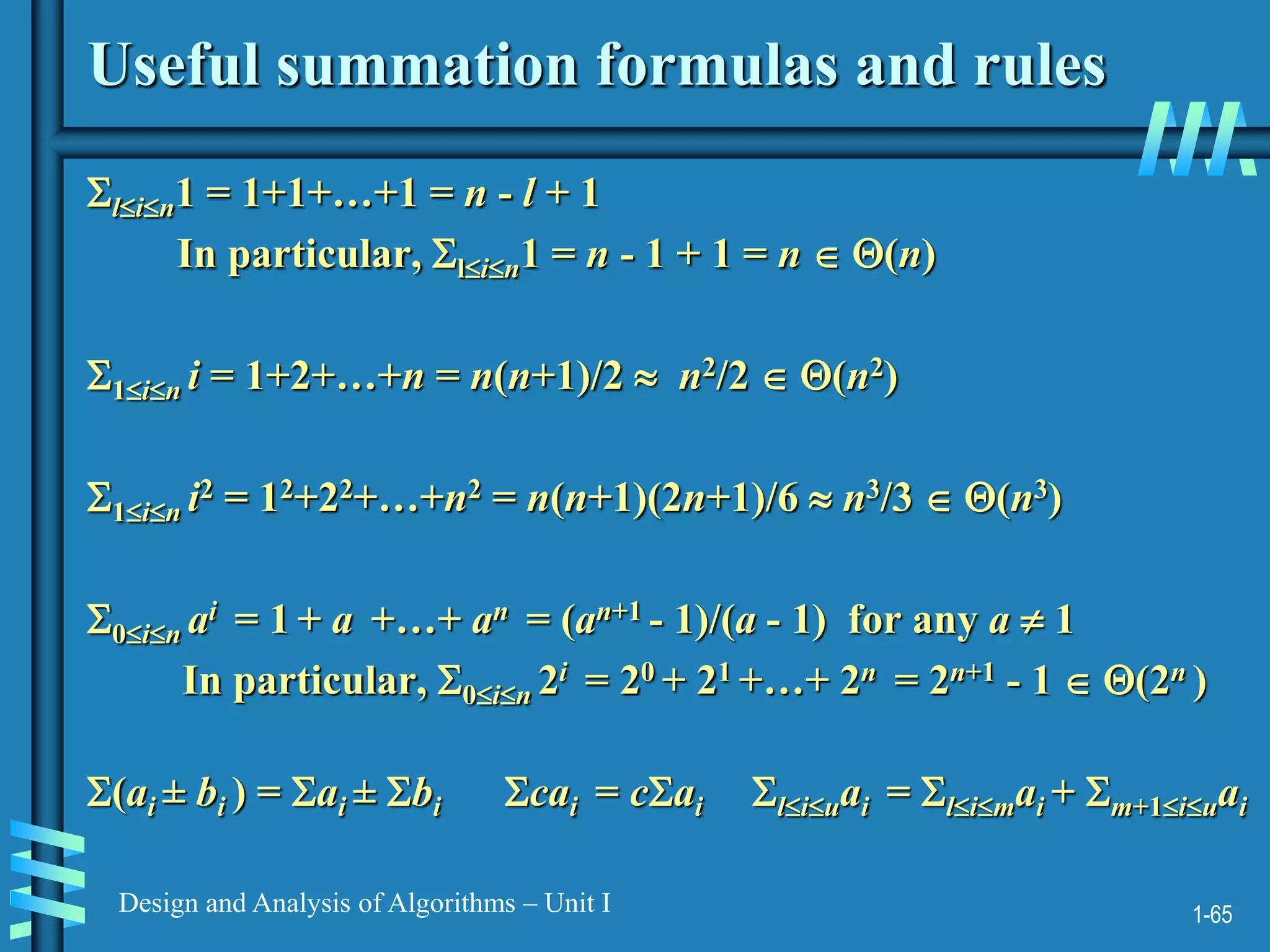
Useful summation formulas and rules
lin1 = 1+1+…+1 = n - l + 1
In particular, lin1 = n - 1 + 1 = n (n)
1in i = 1+2+…+n = n(n+1)/2 n2/2 (n2)
1in i2 = 12+22+…+n2 = n(n+1)(2n+1)/6 n3/3 (n3)
0in ai = 1 + a +…+ an = (an+1 - 1)/(a - 1) for any a 1
In particular, 0in 2i = 20 + 21 +…+ 2n = 2n+1 - 1 (2n )
(ai ± bi ) = ai ± bi cai = cai liuai = limai + m+1iuai
67.
1-66
Design and Analysisof Algorithms – Unit I
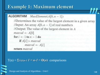
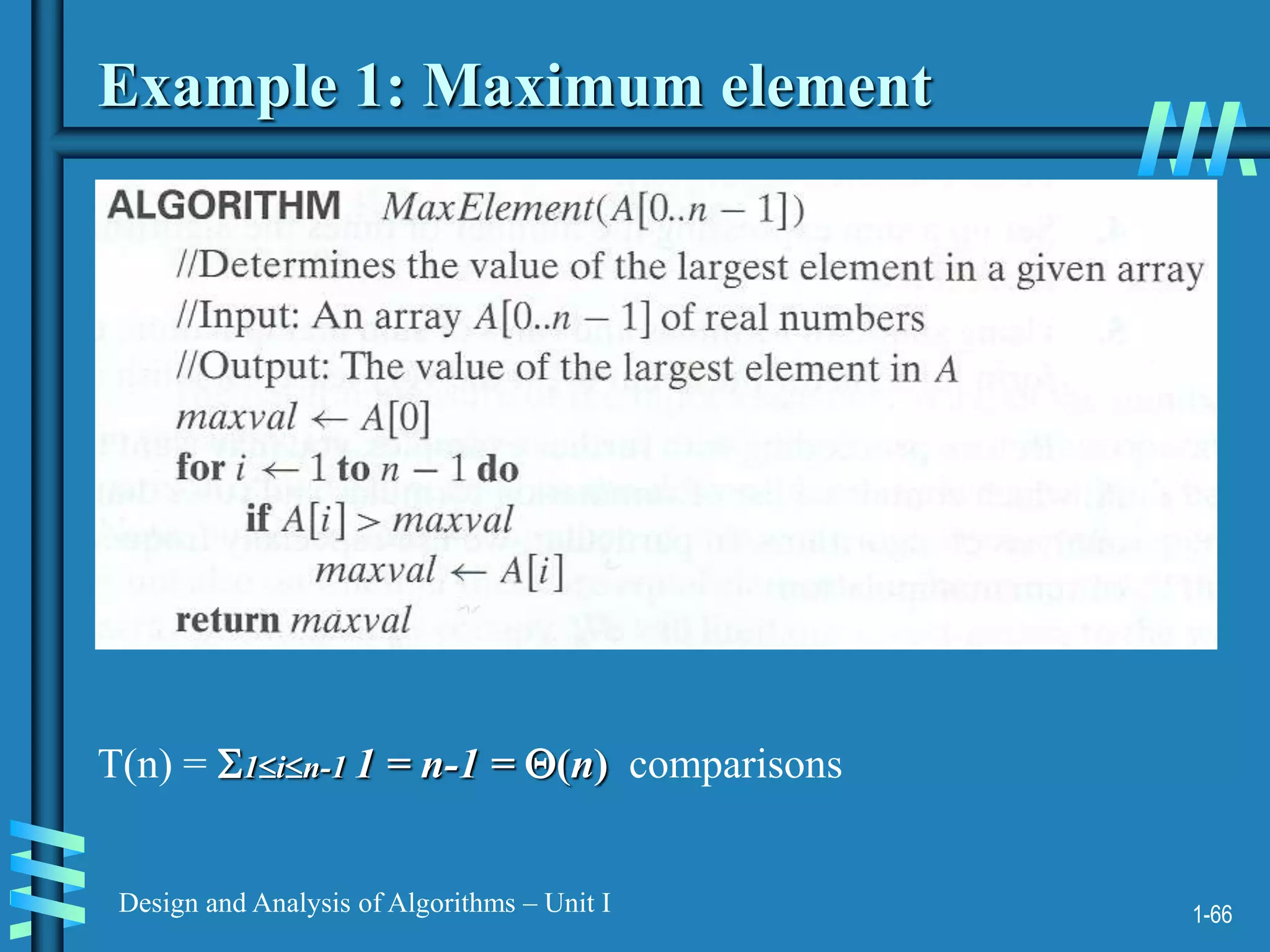
Example 1: Maximum element
T(n) = 1in-1 1 = n-1 = (n) comparisons
68.
1-67
Design and Analysisof Algorithms – Unit I
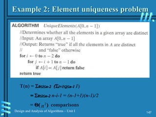
Example 2: Element uniqueness problem
T(n) = 0in-2 (i+1jn-1 1)
= 0in-2 n-i-1 = (n-1+1)(n-1)/2
= ( ) comparisons
2
n
69.
1-68
Design and Analysisof Algorithms – Unit I
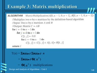
Example 3: Matrix multiplication
T(n) = 0in-1 0in-1 n
= 0in-1 ( )
= ( ) multiplications
2
n
3
n
70.
1-69
Design and Analysisof Algorithms – Unit I
Example 4: Gaussian elimination
Algorithm GaussianElimination(A[0..n-1,0..n])
//Implements Gaussian elimination on an n-by-(n+1) matrix A
for i 0 to n - 2 do
for j i + 1 to n - 1 do
for k i to n do
A[j,k] A[j,k] - A[i,k] A[j,i] / A[i,i]
Find the efficiency class and a constant factor improvement.
for i 0 to n - 2 do
for j i + 1 to n - 1 do
B A[j,i] / A[i,i]
for k i to n do
A[j,k] A[j,k] – A[i,k] * B
1-71
Design and Analysisof Algorithms – Unit I
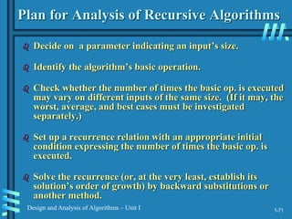
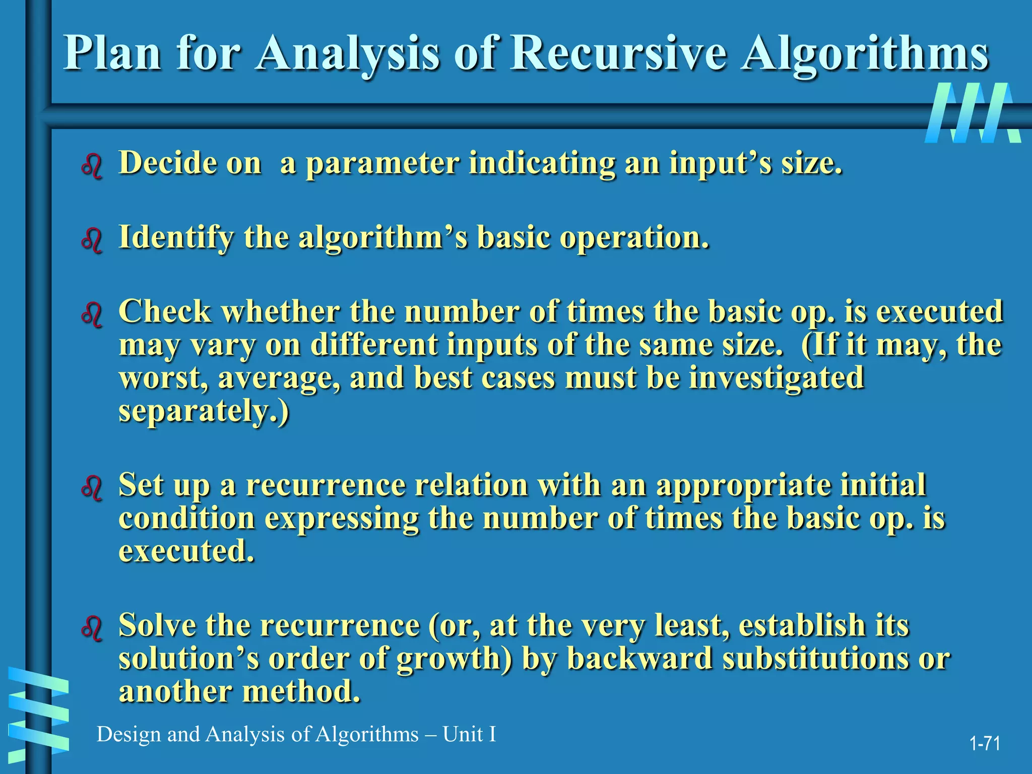
Plan for Analysis of Recursive Algorithms
Decide on a parameter indicating an input’s size.
Identify the algorithm’s basic operation.
Check whether the number of times the basic op. is executed
may vary on different inputs of the same size. (If it may, the
worst, average, and best cases must be investigated
separately.)
Set up a recurrence relation with an appropriate initial
condition expressing the number of times the basic op. is
executed.
Solve the recurrence (or, at the very least, establish its
solution’s order of growth) by backward substitutions or
another method.
73.
1-72
Design and Analysisof Algorithms – Unit I
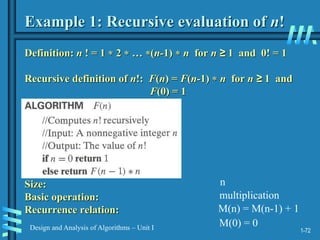
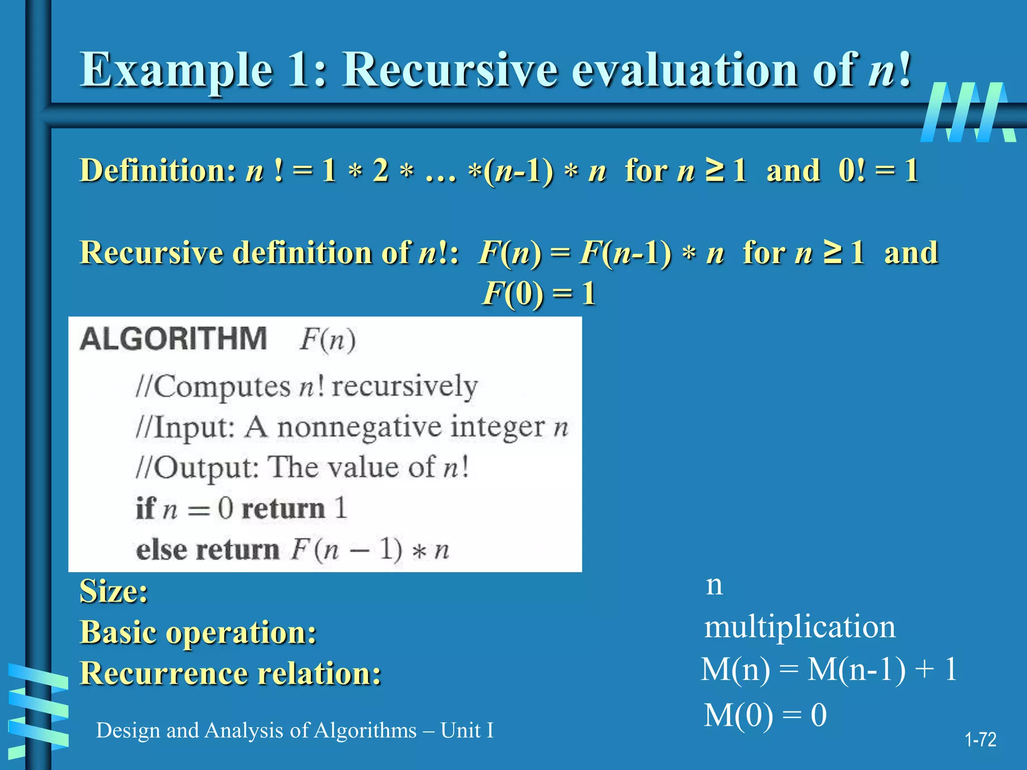
Example 1: Recursive evaluation of n!
Definition: n ! = 1 2 … (n-1) n for n ≥ 1 and 0! = 1
Recursive definition of n!: F(n) = F(n-1) n for n ≥ 1 and
F(0) = 1
Size:
Basic operation:
Recurrence relation:
n
multiplication
M(n) = M(n-1) + 1
M(0) = 0
74.
1-73
Design and Analysisof Algorithms – Unit I
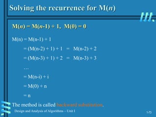
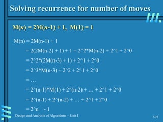
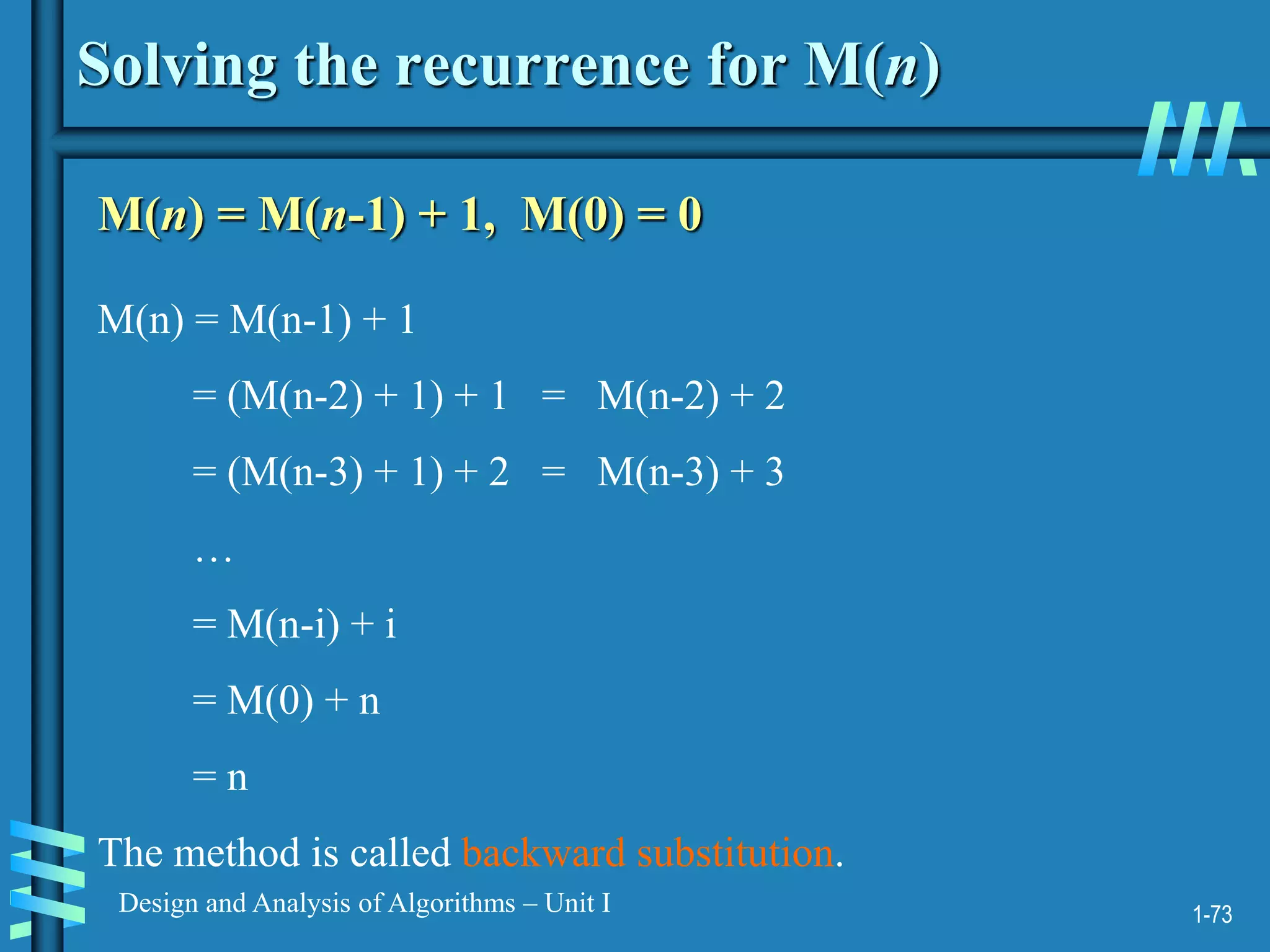
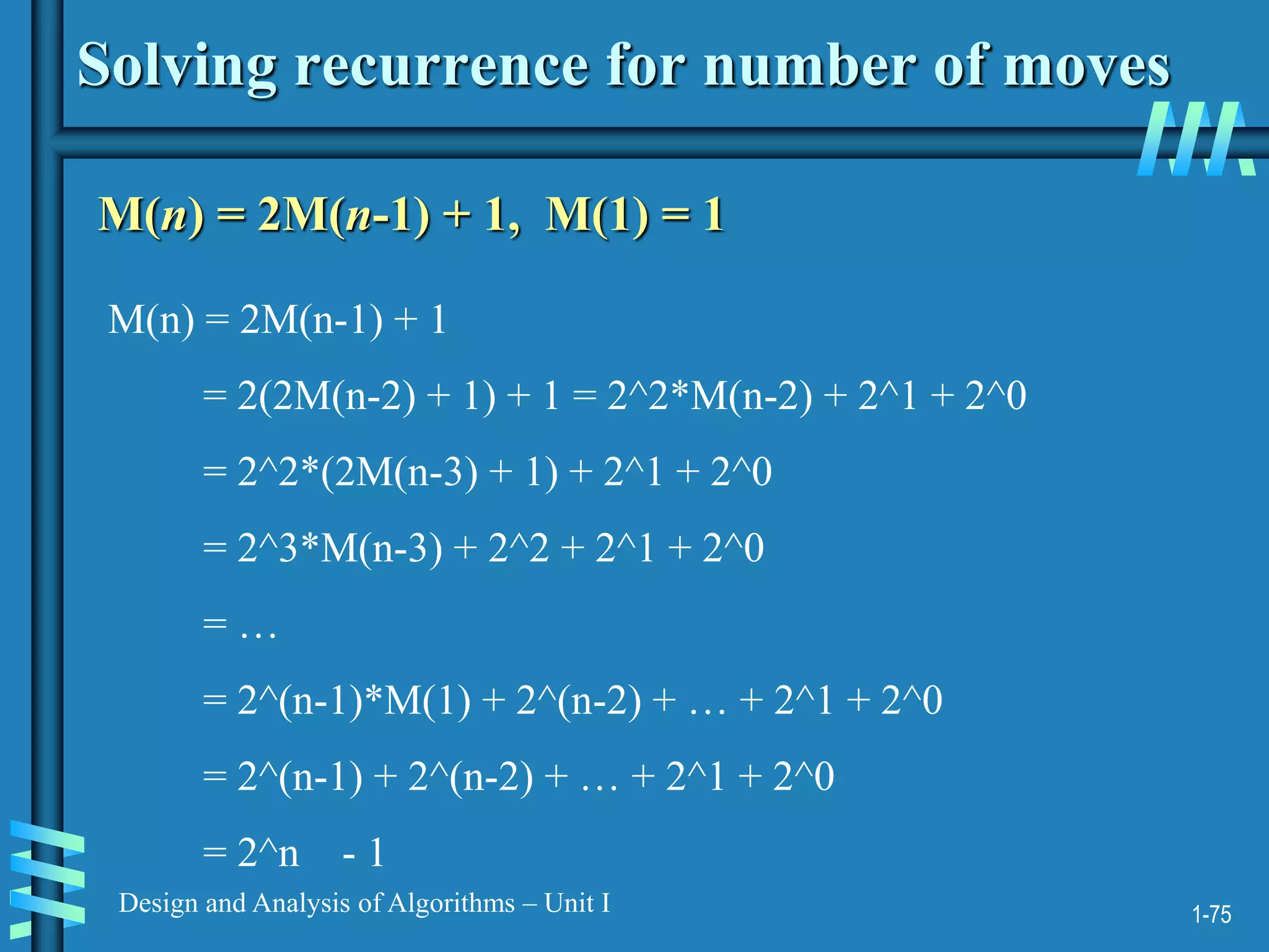
Solving the recurrence for M(n)
M(n) = M(n-1) + 1, M(0) = 0
M(n) = M(n-1) + 1
= (M(n-2) + 1) + 1 = M(n-2) + 2
= (M(n-3) + 1) + 2 = M(n-3) + 3
…
= M(n-i) + i
= M(0) + n
= n
The method is called backward substitution.
75.
1-74
Design and Analysisof Algorithms – Unit I
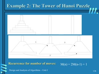
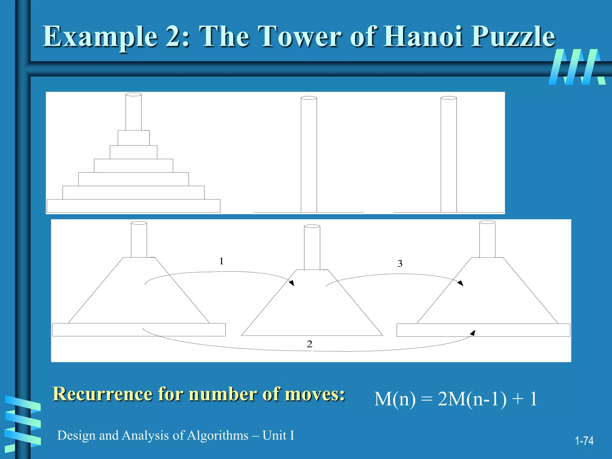
Example 2: The Tower of Hanoi Puzzle
1
2
3
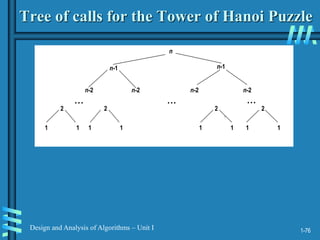
Recurrence for number of moves: M(n) = 2M(n-1) + 1
1-76
Design and Analysisof Algorithms – Unit I
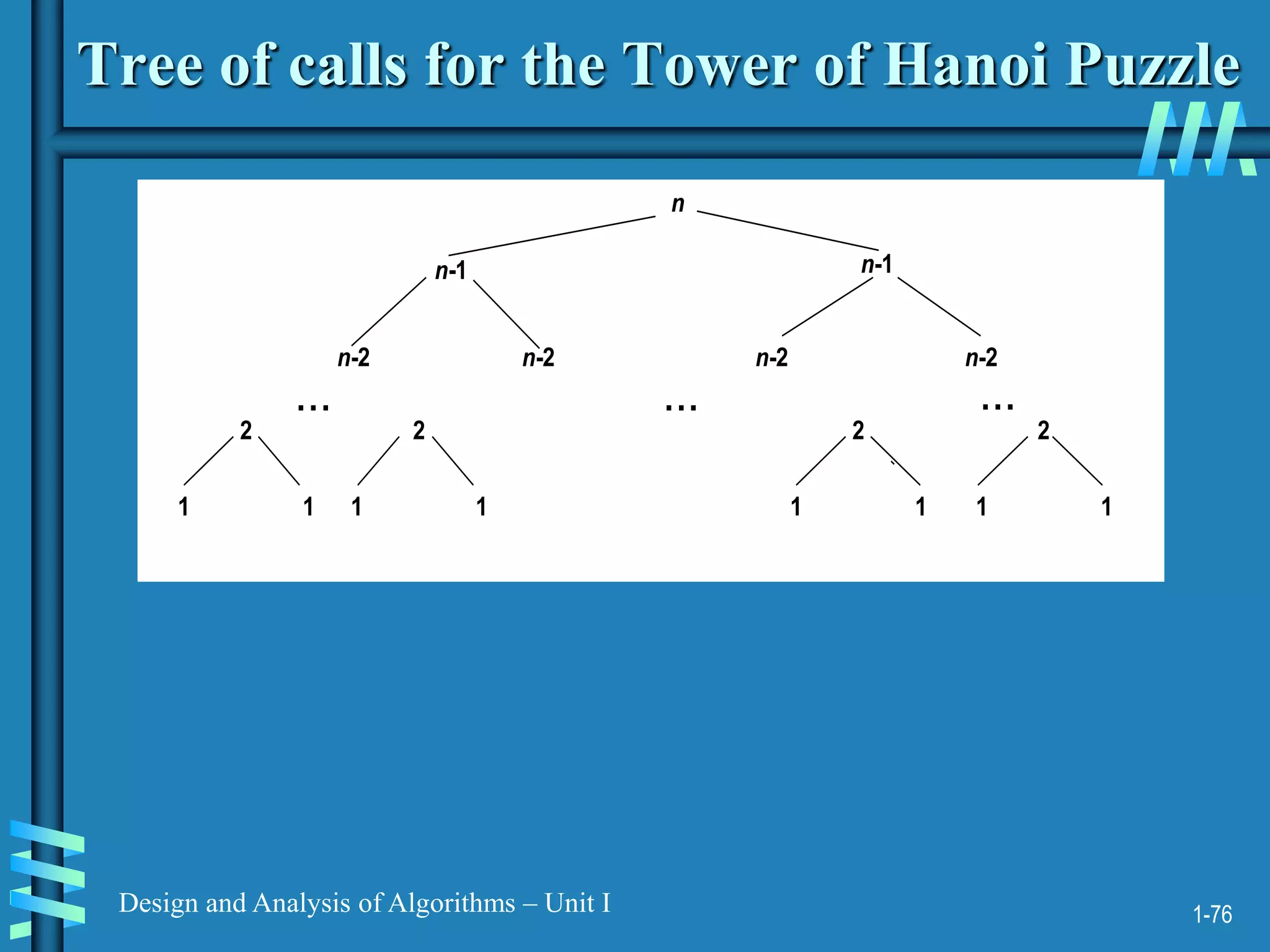
Tree of calls for the Tower of Hanoi Puzzle
n
n-1 n-1
n-2 n-2 n-2 n-2
1 1
... ... ...
2
1 1
2
1 1
2
1 1
2
78.
1-77
Design and Analysisof Algorithms – Unit I
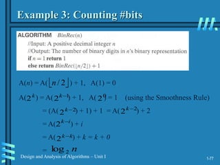
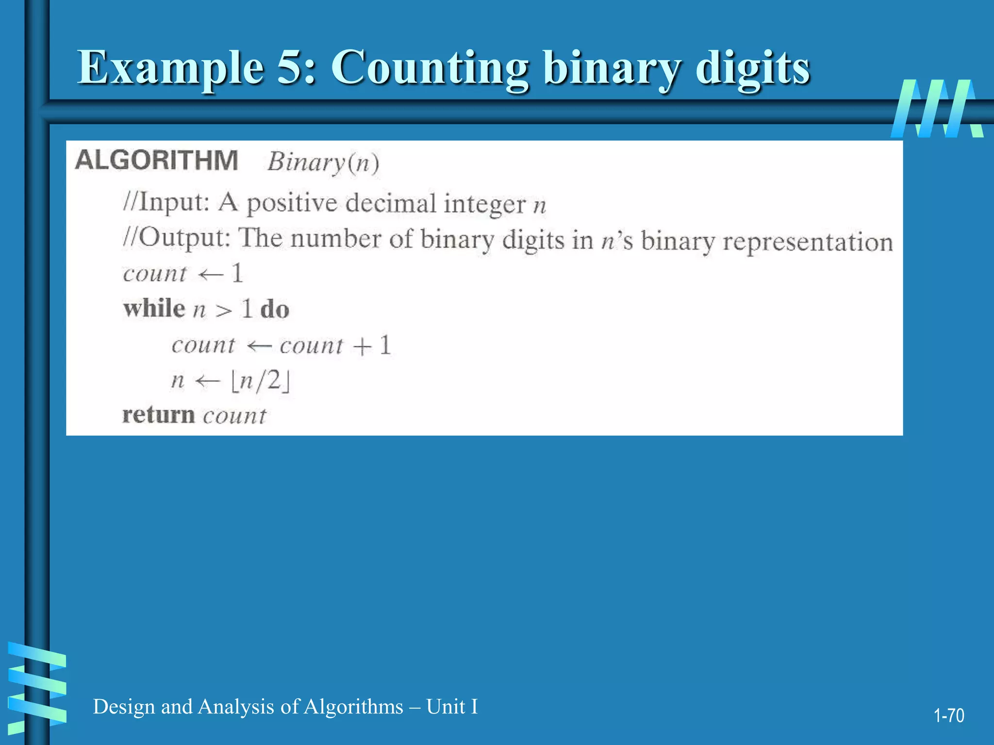
Example 3: Counting #bits
A( ) = A( ) + 1, A( ) = 1 (using the Smoothness Rule)
= (A( ) + 1) + 1 = A( ) + 2
= A( ) + i
= A( ) + k = k + 0
=
k
2 1
2
k 0
2
2
2
k
n
2
log
2
2
k
i
k
2
k
k
2
A(n) = A( ) + 1, A(1) = 0
2
/
n


![1-11
Design and Analysis of Algorithms – Unit I
Other methods for gcd(m,n) [cont.]
Middle-school procedure
Step 1 Find the prime factorization of m
Step 2 Find the prime factorization of n
Step 3 Find all the common prime factors
Step 4 Compute the product of all the common prime factors
and return it as gcd(m,n)
Is this an algorithm?](https://image.slidesharecdn.com/analysis-and-design-of-algorithm-230212162018-f2bb9413/85/ANALYSIS-AND-DESIGN-OF-ALGORITHM-ppt-12-320.jpg)
![1-12
Design and Analysis of Algorithms – Unit I
Sieve of Eratosthenes
Input: Integer n ≥ 2
Output: List of primes less than or equal to n
for p ← 2 to n do A[p] ← p
for p ← 2 to n do
if A[p] 0 //p hasn’t been previously eliminated from the list
j ← p* p
while j ≤ n do
A[j] ← 0 //mark element as eliminated
j ← j + p
Example: 2 3 4 5 6 7 8 9 10 11 12 13 14 15 16 17 18 19 20](https://image.slidesharecdn.com/analysis-and-design-of-algorithm-230212162018-f2bb9413/85/ANALYSIS-AND-DESIGN-OF-ALGORITHM-ppt-13-320.jpg)


![1-69
Design and Analysis of Algorithms – Unit I
Example 4: Gaussian elimination
Algorithm GaussianElimination(A[0..n-1,0..n])
//Implements Gaussian elimination on an n-by-(n+1) matrix A
for i 0 to n - 2 do
for j i + 1 to n - 1 do
for k i to n do
A[j,k] A[j,k] - A[i,k] A[j,i] / A[i,i]
Find the efficiency class and a constant factor improvement.
for i 0 to n - 2 do
for j i + 1 to n - 1 do
B A[j,i] / A[i,i]
for k i to n do
A[j,k] A[j,k] – A[i,k] * B](https://image.slidesharecdn.com/analysis-and-design-of-algorithm-230212162018-f2bb9413/85/ANALYSIS-AND-DESIGN-OF-ALGORITHM-ppt-70-320.jpg)


![1-11
Design and Analysis of Algorithms – Unit I
Other methods for gcd(m,n) [cont.]
Middle-school procedure
Step 1 Find the prime factorization of m
Step 2 Find the prime factorization of n
Step 3 Find all the common prime factors
Step 4 Compute the product of all the common prime factors
and return it as gcd(m,n)
Is this an algorithm?](https://image.slidesharecdn.com/analysis-and-design-of-algorithm-230212162018-f2bb9413/75/ANALYSIS-AND-DESIGN-OF-ALGORITHM-ppt-12-2048.jpg)
![1-12
Design and Analysis of Algorithms – Unit I
Sieve of Eratosthenes
Input: Integer n ≥ 2
Output: List of primes less than or equal to n
for p ← 2 to n do A[p] ← p
for p ← 2 to n do
if A[p] 0 //p hasn’t been previously eliminated from the list
j ← p* p
while j ≤ n do
A[j] ← 0 //mark element as eliminated
j ← j + p
Example: 2 3 4 5 6 7 8 9 10 11 12 13 14 15 16 17 18 19 20](https://image.slidesharecdn.com/analysis-and-design-of-algorithm-230212162018-f2bb9413/75/ANALYSIS-AND-DESIGN-OF-ALGORITHM-ppt-13-2048.jpg)


![1-69
Design and Analysis of Algorithms – Unit I
Example 4: Gaussian elimination
Algorithm GaussianElimination(A[0..n-1,0..n])
//Implements Gaussian elimination on an n-by-(n+1) matrix A
for i 0 to n - 2 do
for j i + 1 to n - 1 do
for k i to n do
A[j,k] A[j,k] - A[i,k] A[j,i] / A[i,i]
Find the efficiency class and a constant factor improvement.
for i 0 to n - 2 do
for j i + 1 to n - 1 do
B A[j,i] / A[i,i]
for k i to n do
A[j,k] A[j,k] – A[i,k] * B](https://image.slidesharecdn.com/analysis-and-design-of-algorithm-230212162018-f2bb9413/75/ANALYSIS-AND-DESIGN-OF-ALGORITHM-ppt-70-2048.jpg)


![Data Structures - Lecture 8 [Sorting Algorithms]](https://cdn.slidesharecdn.com/ss_thumbnails/lecture-8sortingalgorithms-150205105023-conversion-gate02-thumbnail.jpg?width=600ounds&width=560&fit=bounds)


![[Make a Copy] Region - Team Name - Project Name.pptx](https://cdn.slidesharecdn.com/ss_thumbnails/makeacopyregion-teamname-projectname-230502014105-e31b8a52-thumbnail.jpg?width=600ounds&width=560&fit=bounds)


