Downloaded 3,736 times


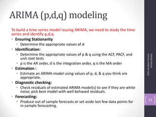


![Autocorrelation Function (ACF)
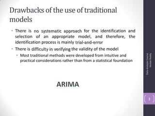
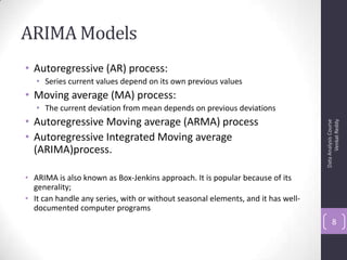
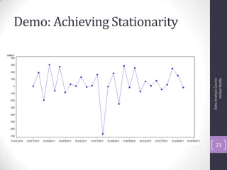
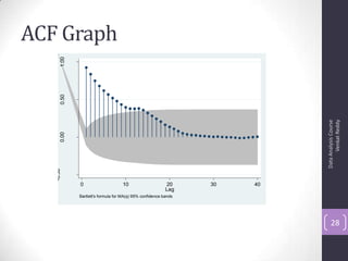
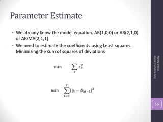
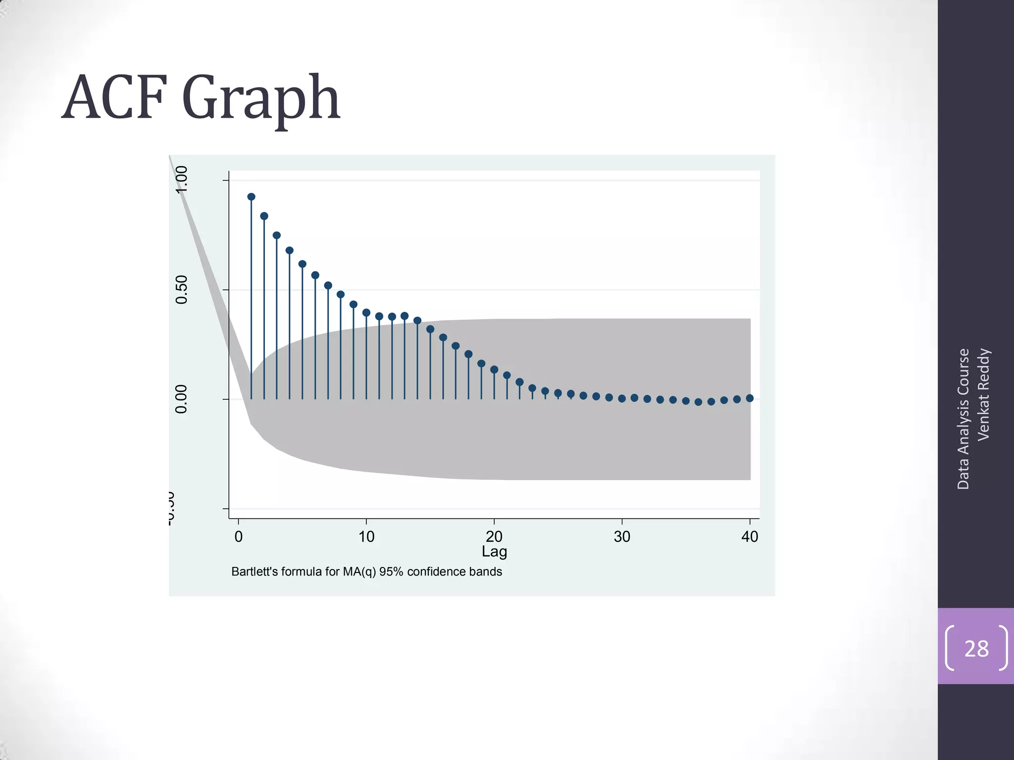
• Autocorrelation is a correlation coefficient. However, instead
of correlation between two different variables, the correlation
is between two values of the same variable at times Xi and
Xi+k.
• Correlation with lag-1, lag2, lag3 etc.,
• The ACF represents the degree of persistence over respective
lags of a variable.
ρk = γk / γ0 = covariance at lag k/ variance
ρk = E[(yt – μ)(yt-k – μ)]2
E[(yt – μ)2]
ACF (0) = 1, ACF (k) = ACF (-k)
DataAnalysisCourse
VenkatReddy
27](https://image.slidesharecdn.com/6-130914140240-phpapp01/85/ARIMA-27-320.jpg)
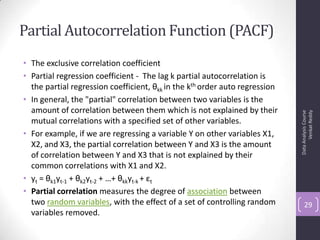
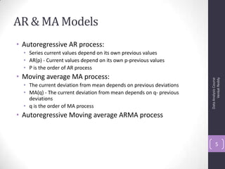
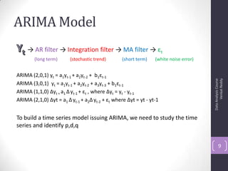
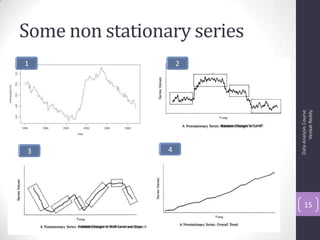
![PACF Graph
DataAnalysisCourse
VenkatReddy
30
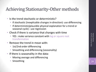
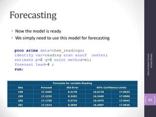
-0.50
0.000.501.00
0 10 20 30 40
Lag
95% Confidence bands [se = 1/sqrt(n)]](https://image.slidesharecdn.com/6-130914140240-phpapp01/85/ARIMA-30-320.jpg)
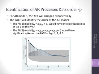


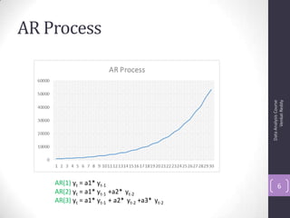
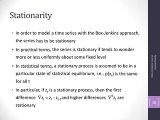
![Autocorrelation Function (ACF)
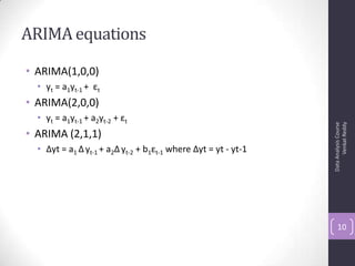
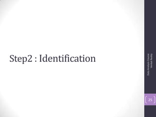
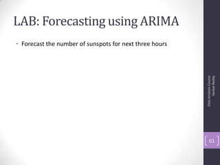
• Autocorrelation is a correlation coefficient. However, instead
of correlation between two different variables, the correlation
is between two values of the same variable at times Xi and
Xi+k.
• Correlation with lag-1, lag2, lag3 etc.,
• The ACF represents the degree of persistence over respective
lags of a variable.
ρk = γk / γ0 = covariance at lag k/ variance
ρk = E[(yt – μ)(yt-k – μ)]2
E[(yt – μ)2]
ACF (0) = 1, ACF (k) = ACF (-k)
DataAnalysisCourse
VenkatReddy
27](https://image.slidesharecdn.com/6-130914140240-phpapp01/75/ARIMA-27-2048.jpg)
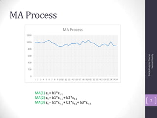
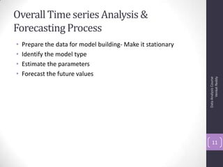
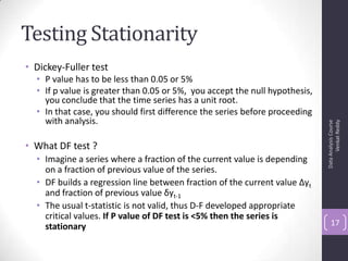
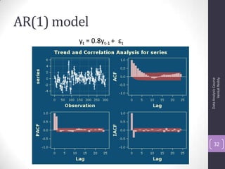
![PACF Graph
DataAnalysisCourse
VenkatReddy
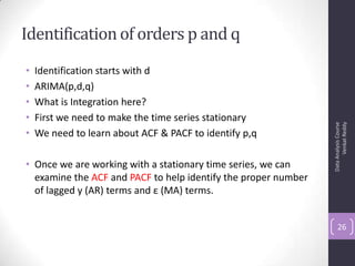
30
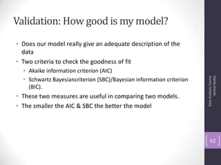
-0.50
0.000.501.00
0 10 20 30 40
Lag
95% Confidence bands [se = 1/sqrt(n)]](https://image.slidesharecdn.com/6-130914140240-phpapp01/75/ARIMA-30-2048.jpg)


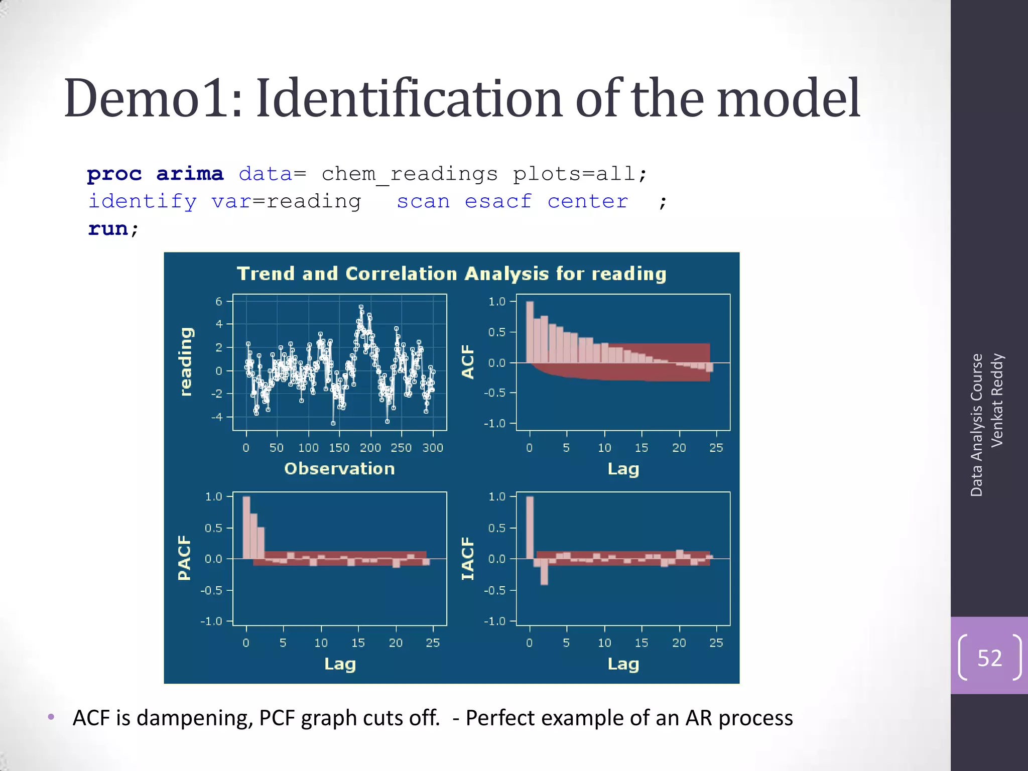
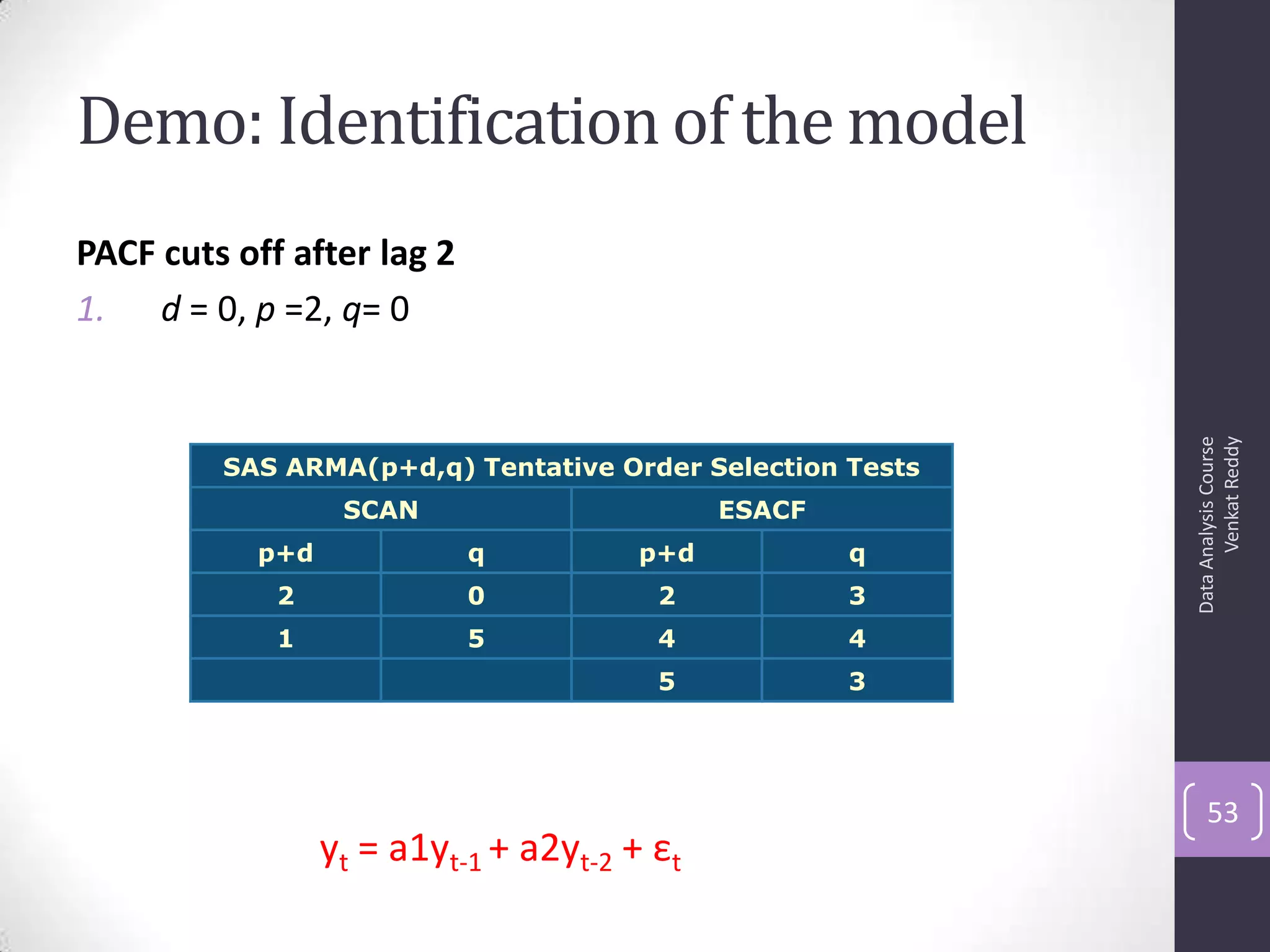
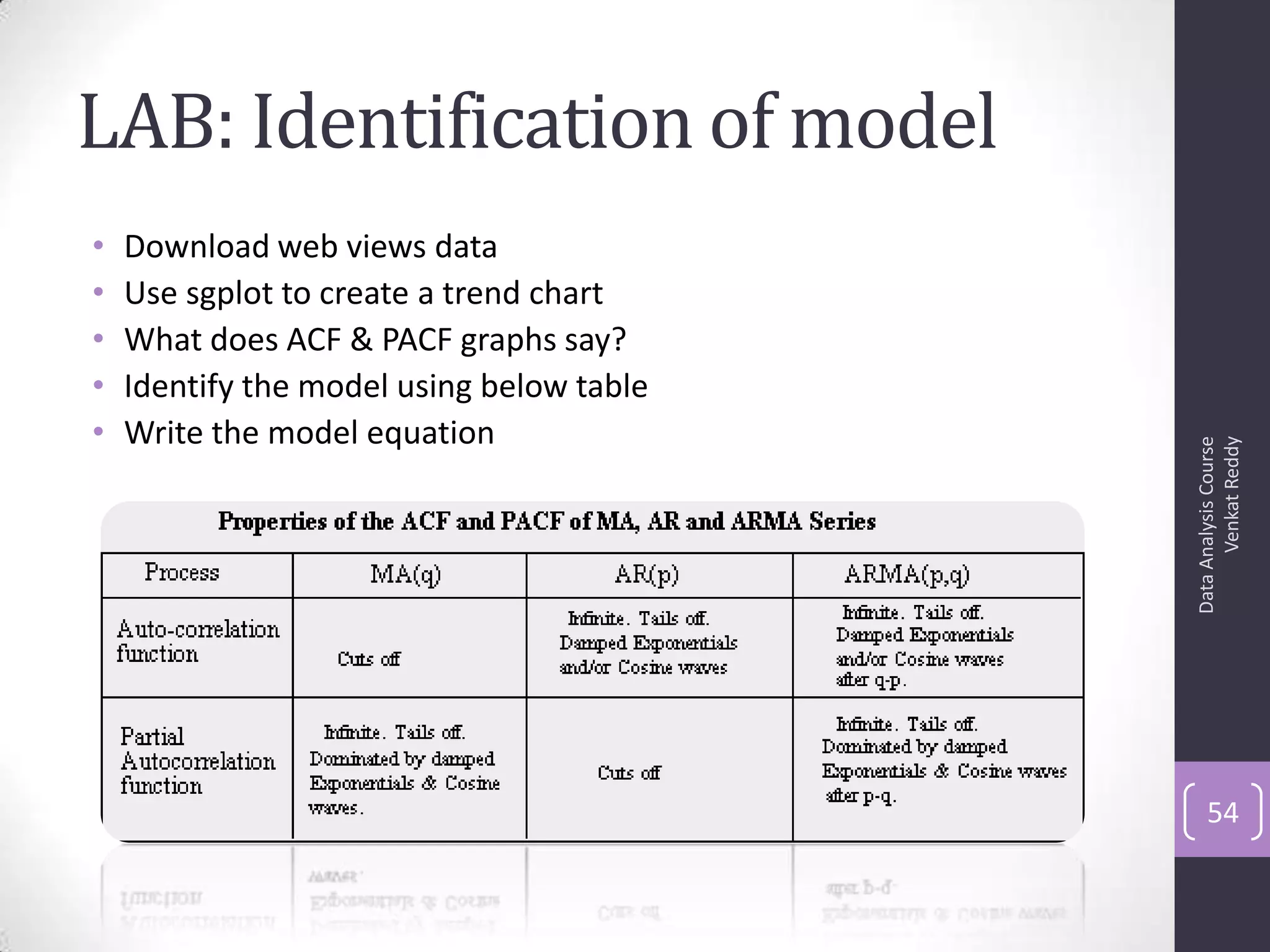


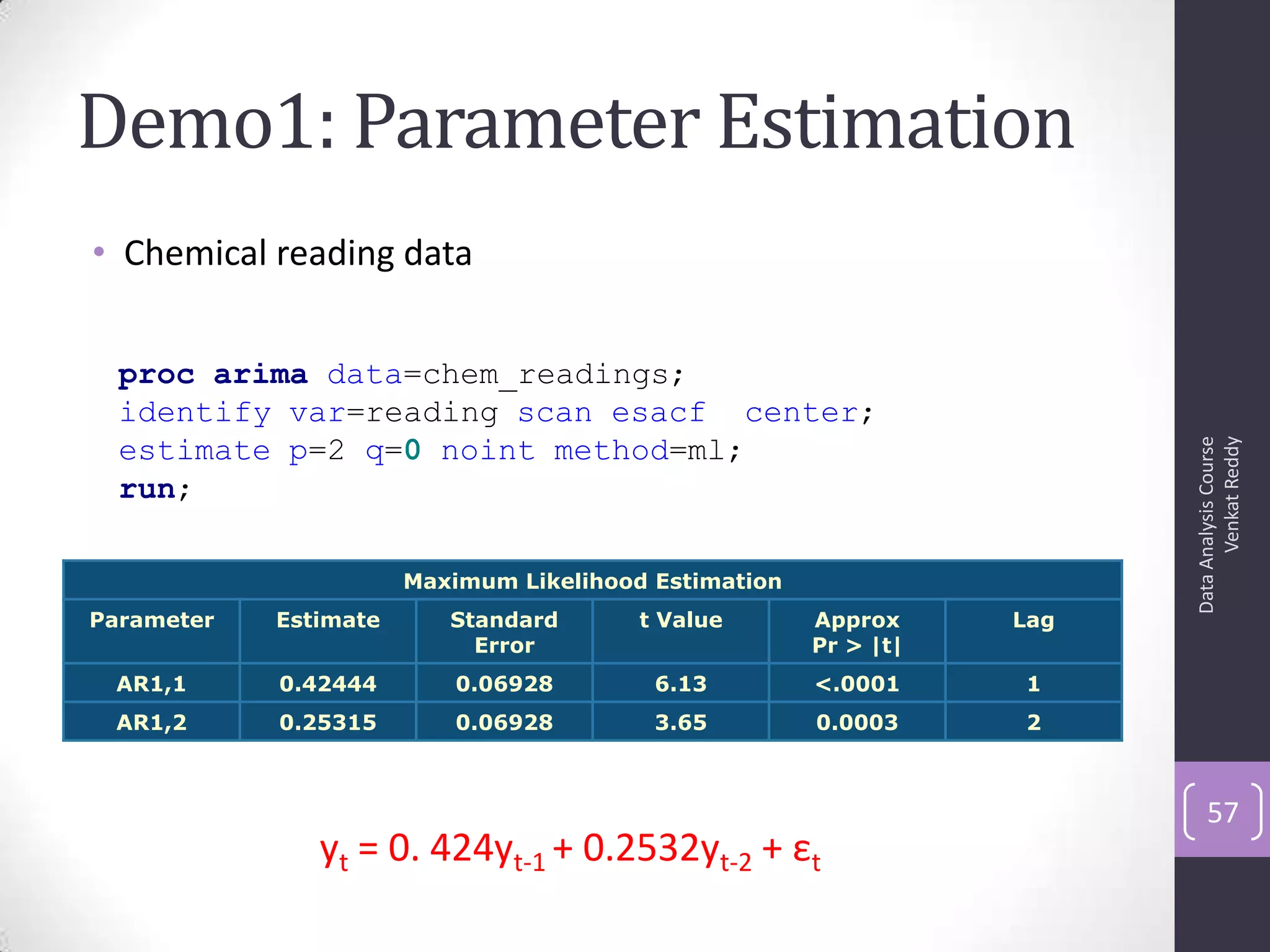


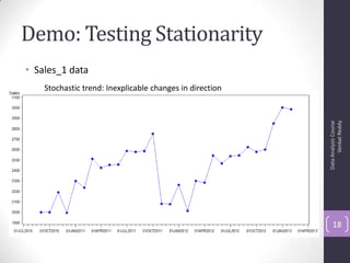
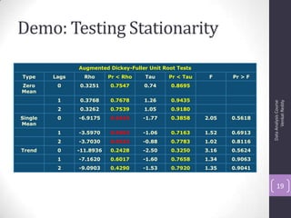
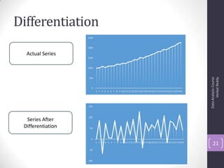
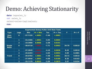
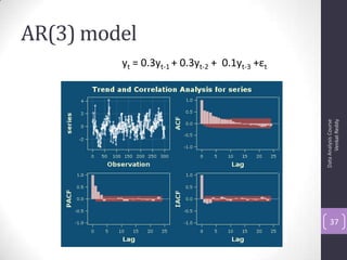
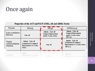
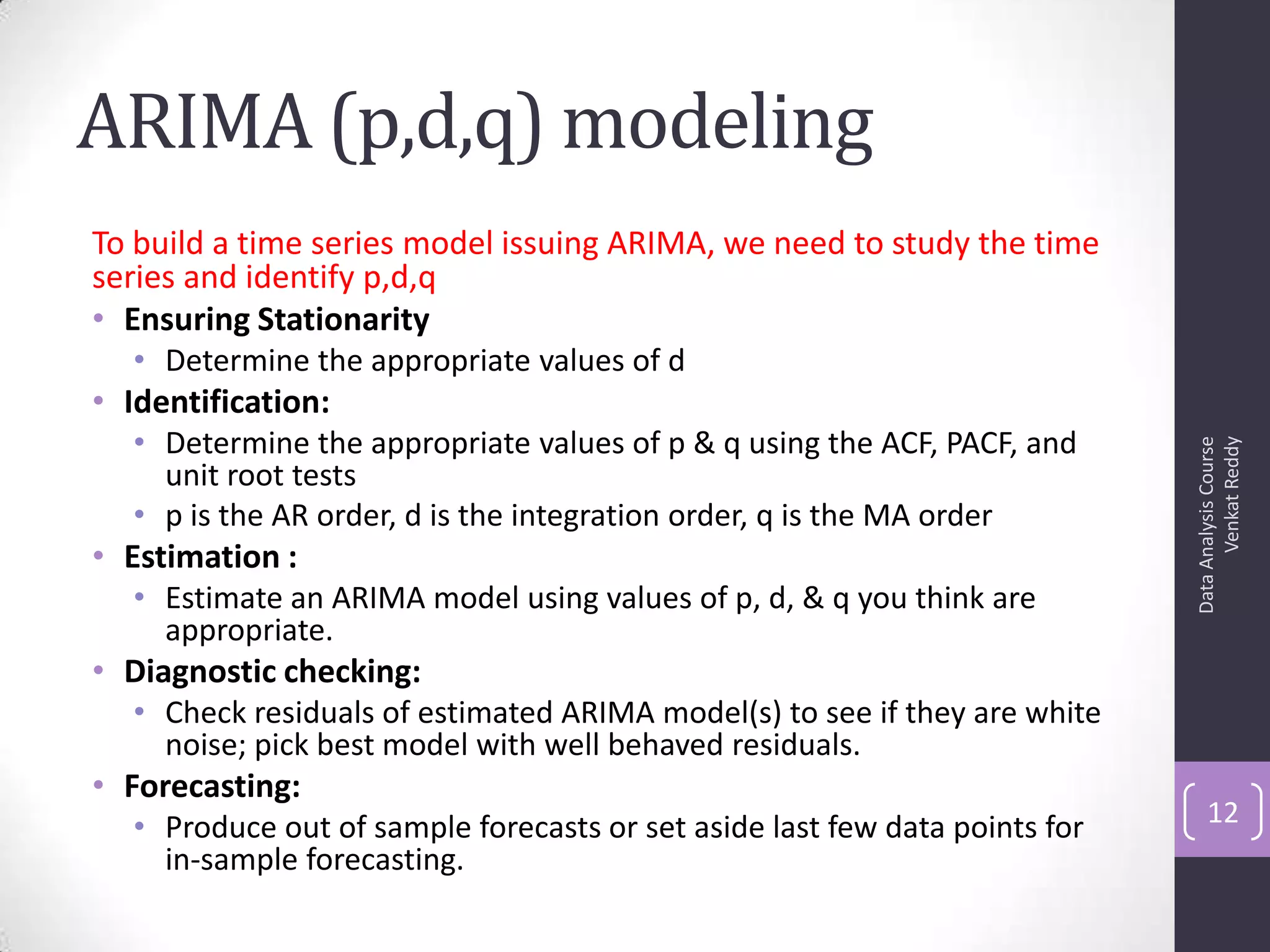
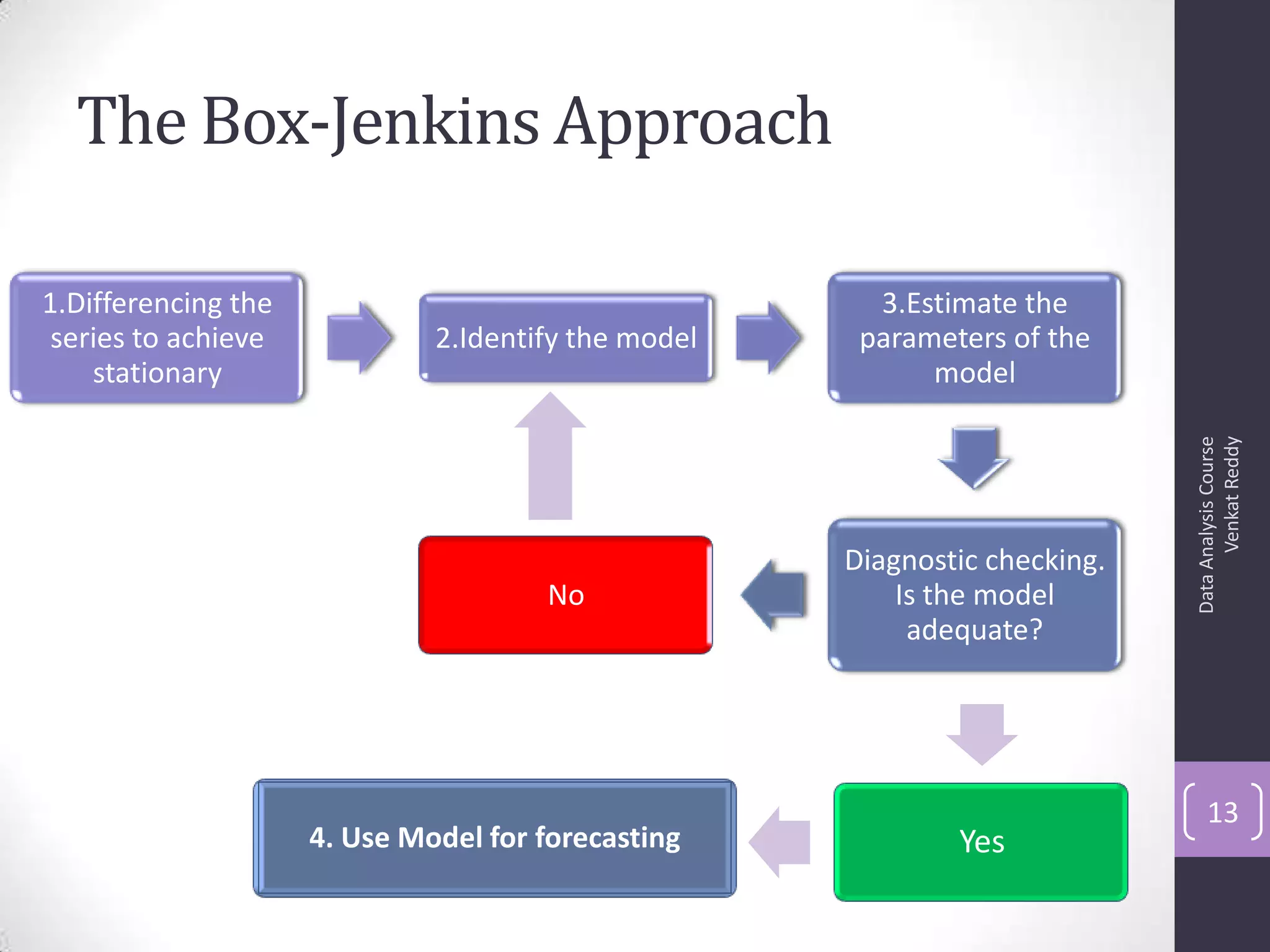
The document discusses time series analysis and forecasting using ARIMA models, focusing on the methodologies for model identification, estimation, and forecasting. It emphasizes the importance of stationarity in time series data and the steps involved in the Box-Jenkins approach, including differencing, model identification through ACF and PACF analysis, and diagnostic checking for model adequacy. Key components such as autoregressive and moving average processes are explained, along with practical guidelines for implementing ARIMA modeling.


