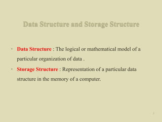
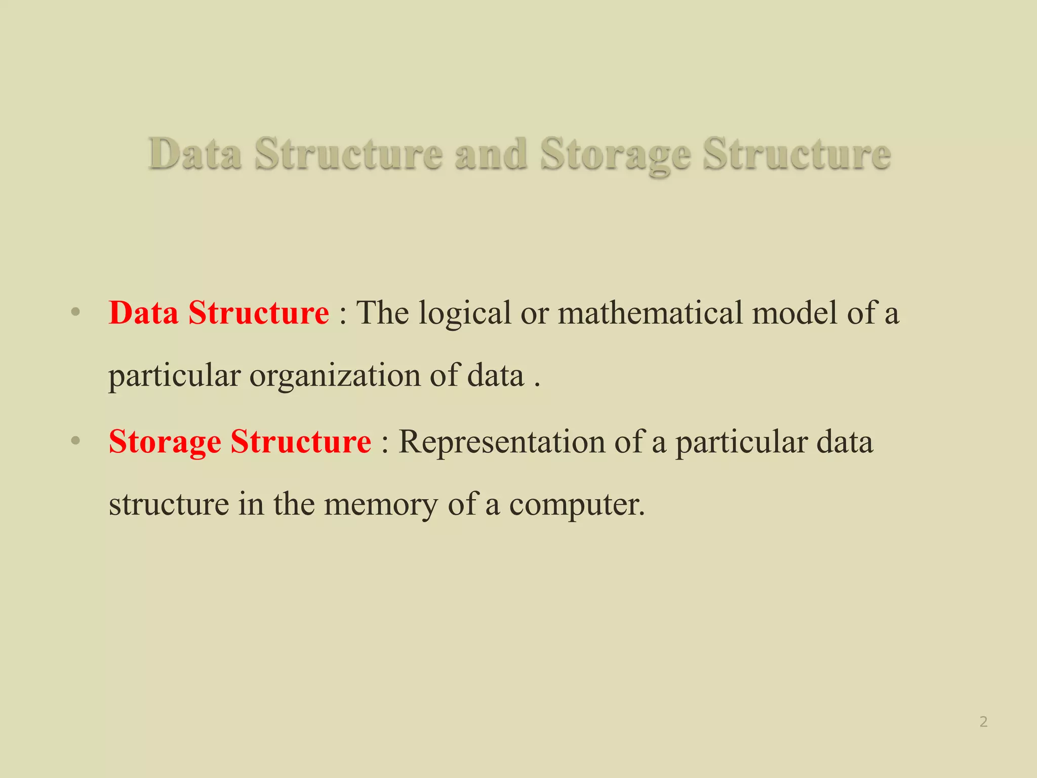
1. The document discusses data structures and their representation in memory. It defines a data structure as a logical organization of data and storage structure as the physical representation of a data structure in computer memory.
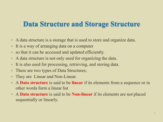
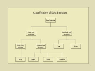
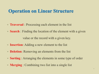
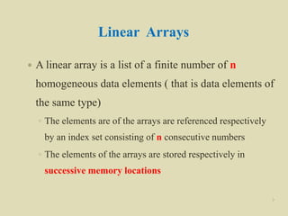
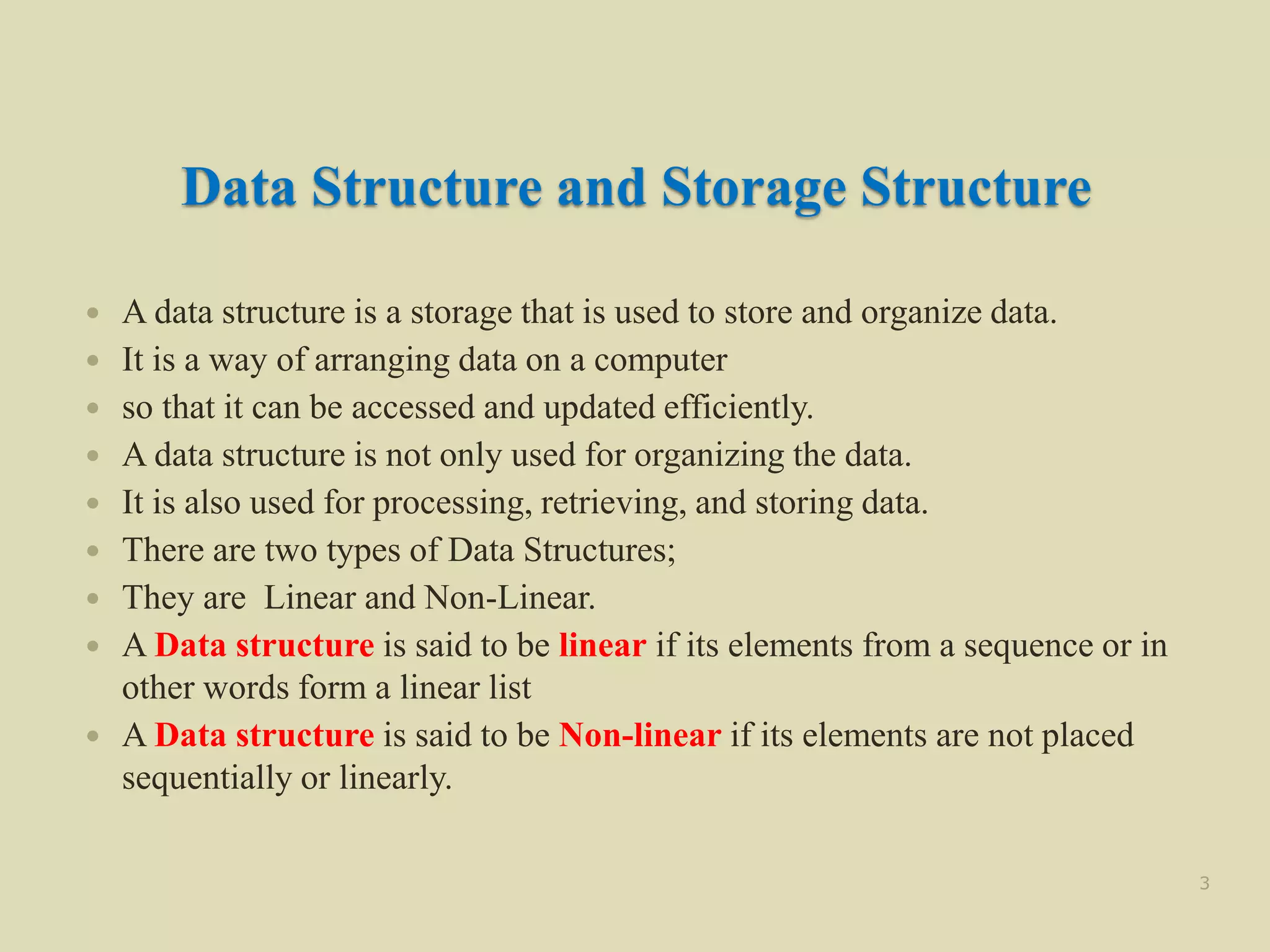
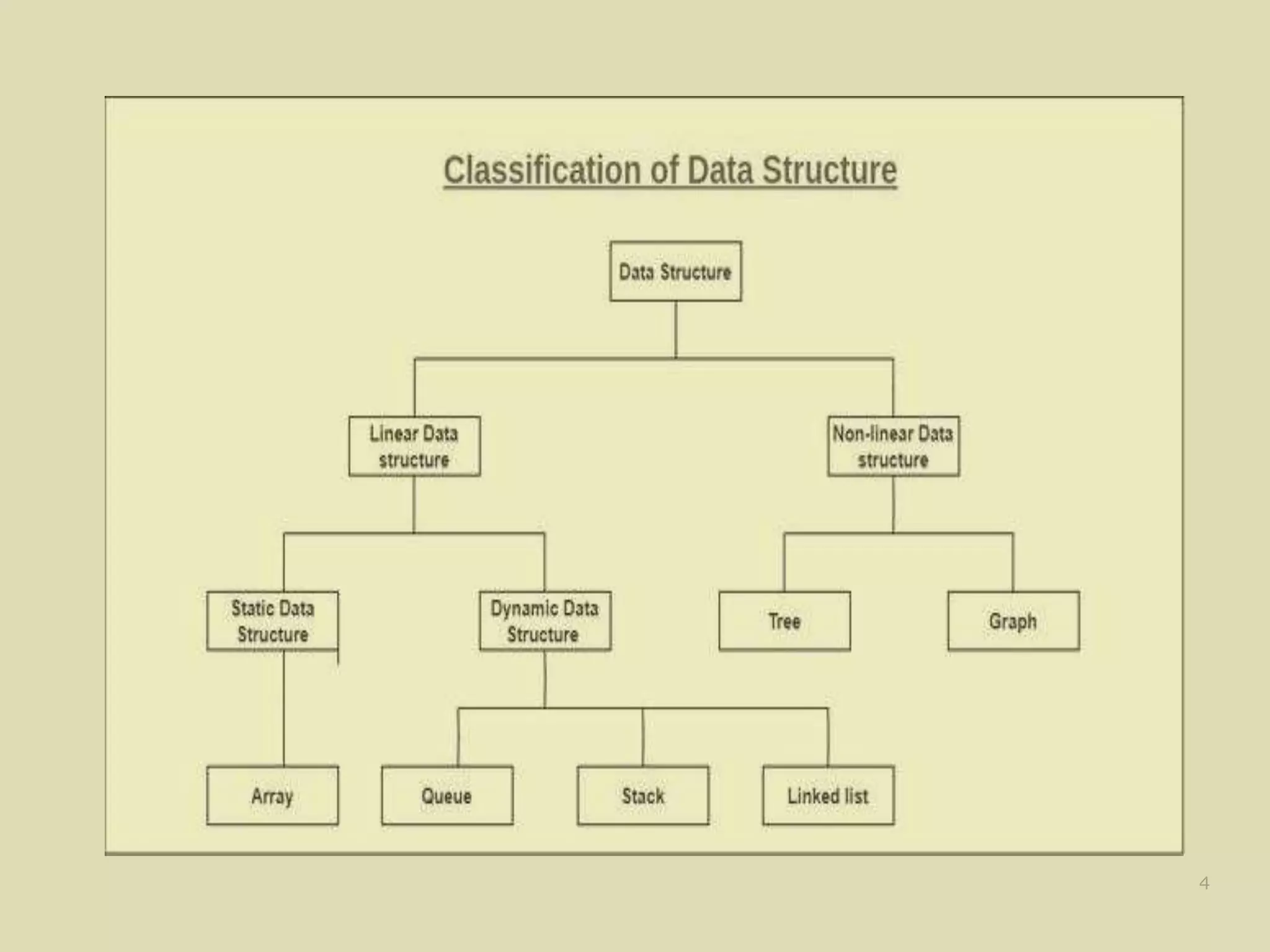
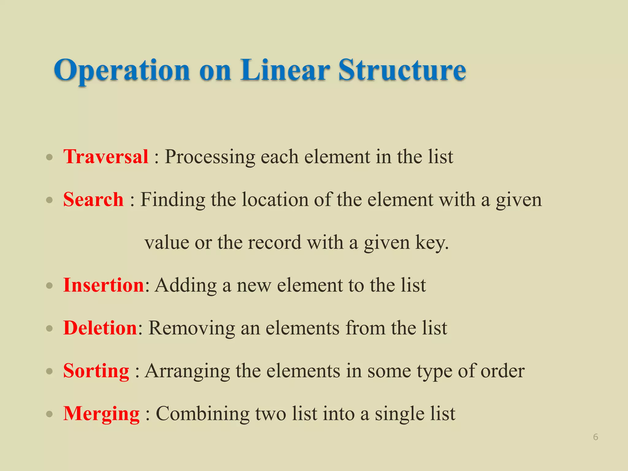
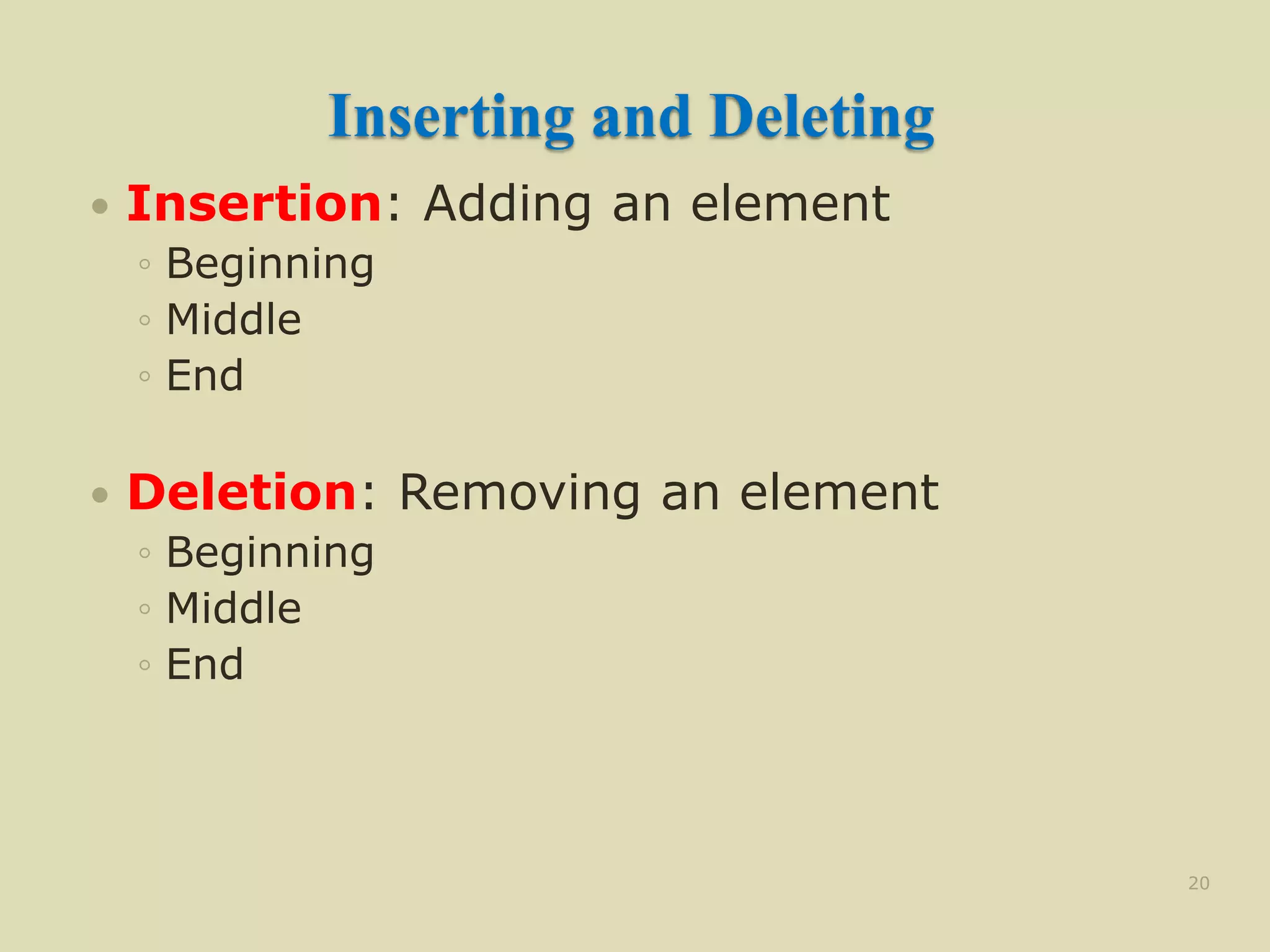
2. Linear and non-linear data structures are described. Linear data structures like arrays have elements arranged sequentially while non-linear structures like linked lists use pointers. Common linear data structure operations like traversal, search, insertion and deletion are also outlined.
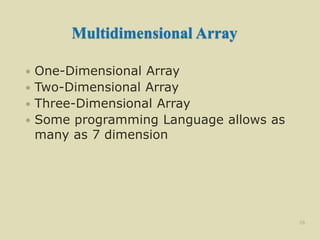
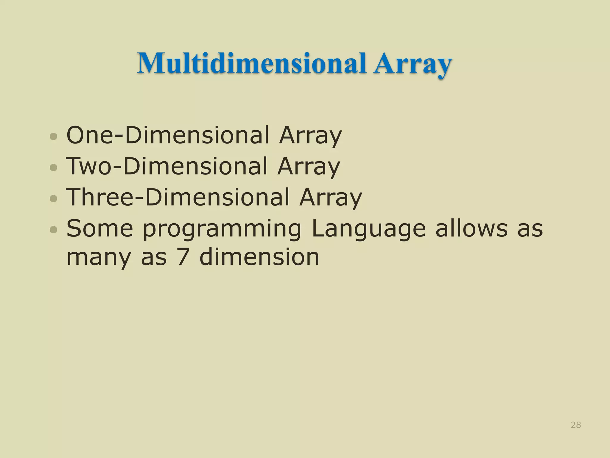
3. The key aspects of one-dimensional and multi-dimensional arrays are covered, including their indexing, memory representation and addressing calculations.

![Representation in Memory
Two basic representation in memory
◦ Have a linear relationship between the elements represented
by means of sequential memory locations [ Arrays]
◦ Have the linear relationship between the elements
represented by means of pointer or links [ Linked List]
5](https://image.slidesharecdn.com/arraysindatastructure-230228062337-a6c22909/85/arrays-in-data-structure-pptx-5-320.jpg)
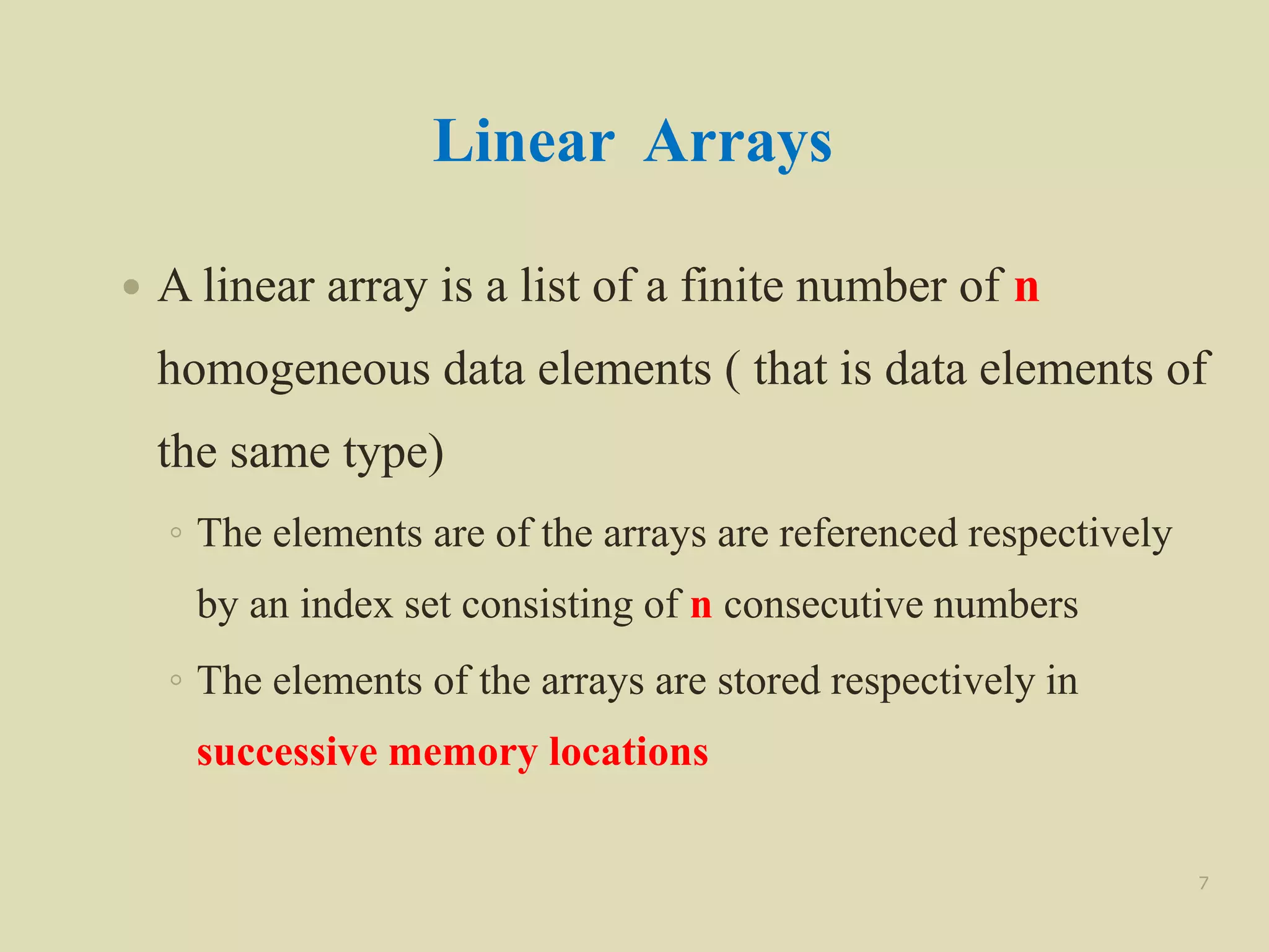
![Linear Arrays
Element of an array A may be denoted by
◦ Subscript notation A1, A2, , …. , An
◦ Parenthesis notation A(1), A(2), …. , A(n)
◦ Bracket notation A[1], A[2], ….. , A[n]
The number K in A[K] is called subscript
or an index and A[K] is called a
subscripted variable
9](https://image.slidesharecdn.com/arraysindatastructure-230228062337-a6c22909/85/arrays-in-data-structure-pptx-9-320.jpg)
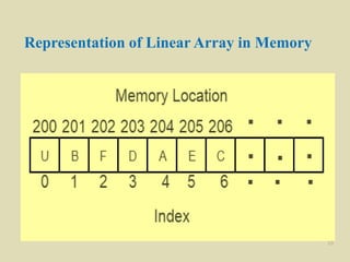
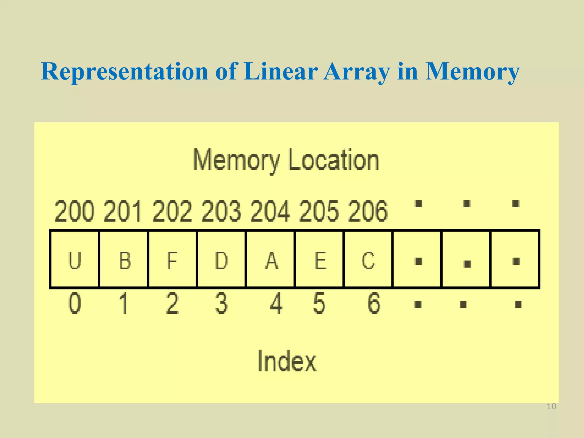
![Representation of Linear Array in Memory
Let LA be a linear array in the memory of the
computer
LOC(LA[K]) = address of the element
LA[K] of the array LA
The element of LA are stored in the
successive memory cells
Computer does not need to keep track of the
address of every element of LA, but need to
track only the address of the first element of
the array denoted by Base(LA) called the
base address of LA
11](https://image.slidesharecdn.com/arraysindatastructure-230228062337-a6c22909/85/arrays-in-data-structure-pptx-11-320.jpg)
![Representation of Linear Array in Memory
LOC(LA[K]) = Base(LA) + w(K – lower
bound) where w is the number of words
per memory cell of the array LA
w is a size of the data type.
12](https://image.slidesharecdn.com/arraysindatastructure-230228062337-a6c22909/85/arrays-in-data-structure-pptx-12-320.jpg)


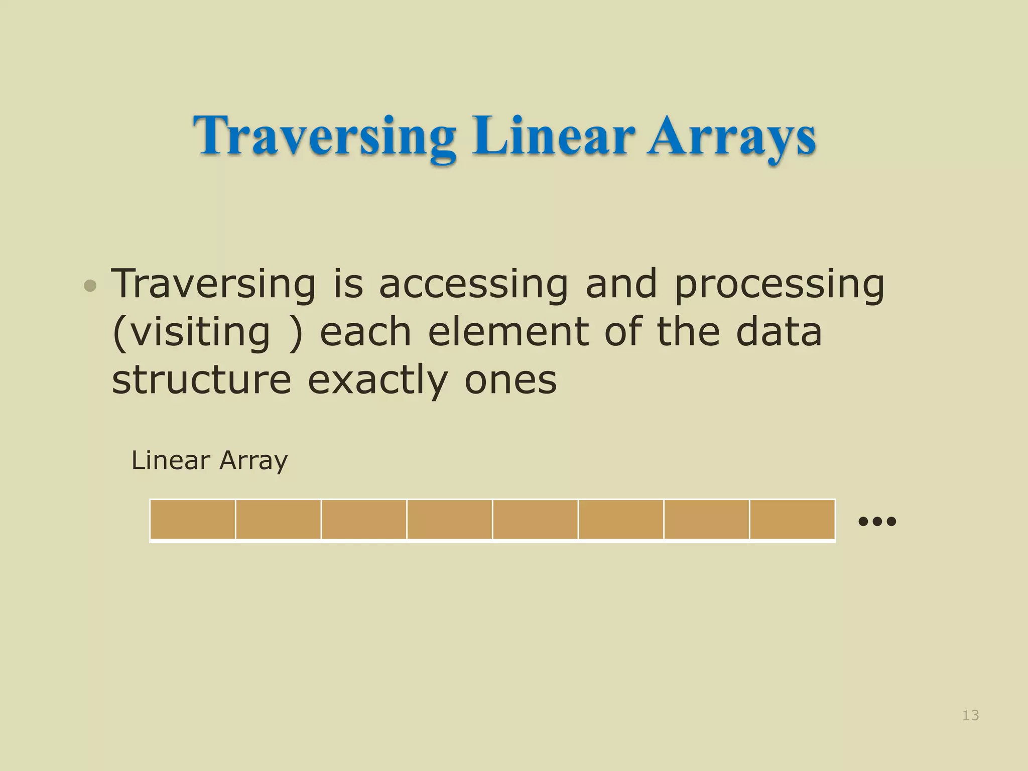
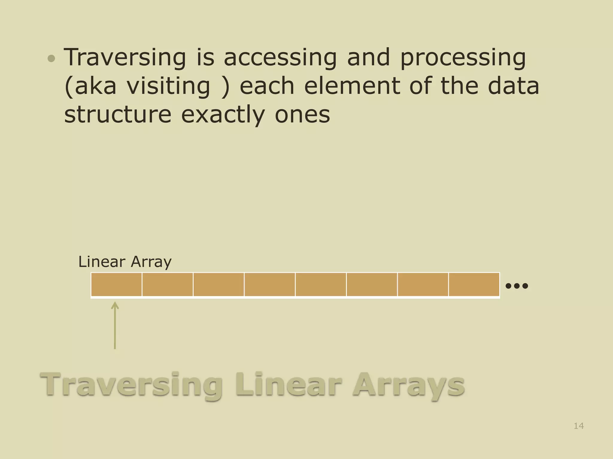
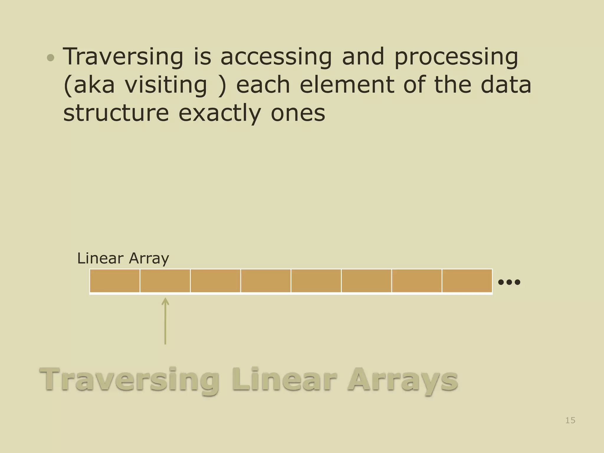
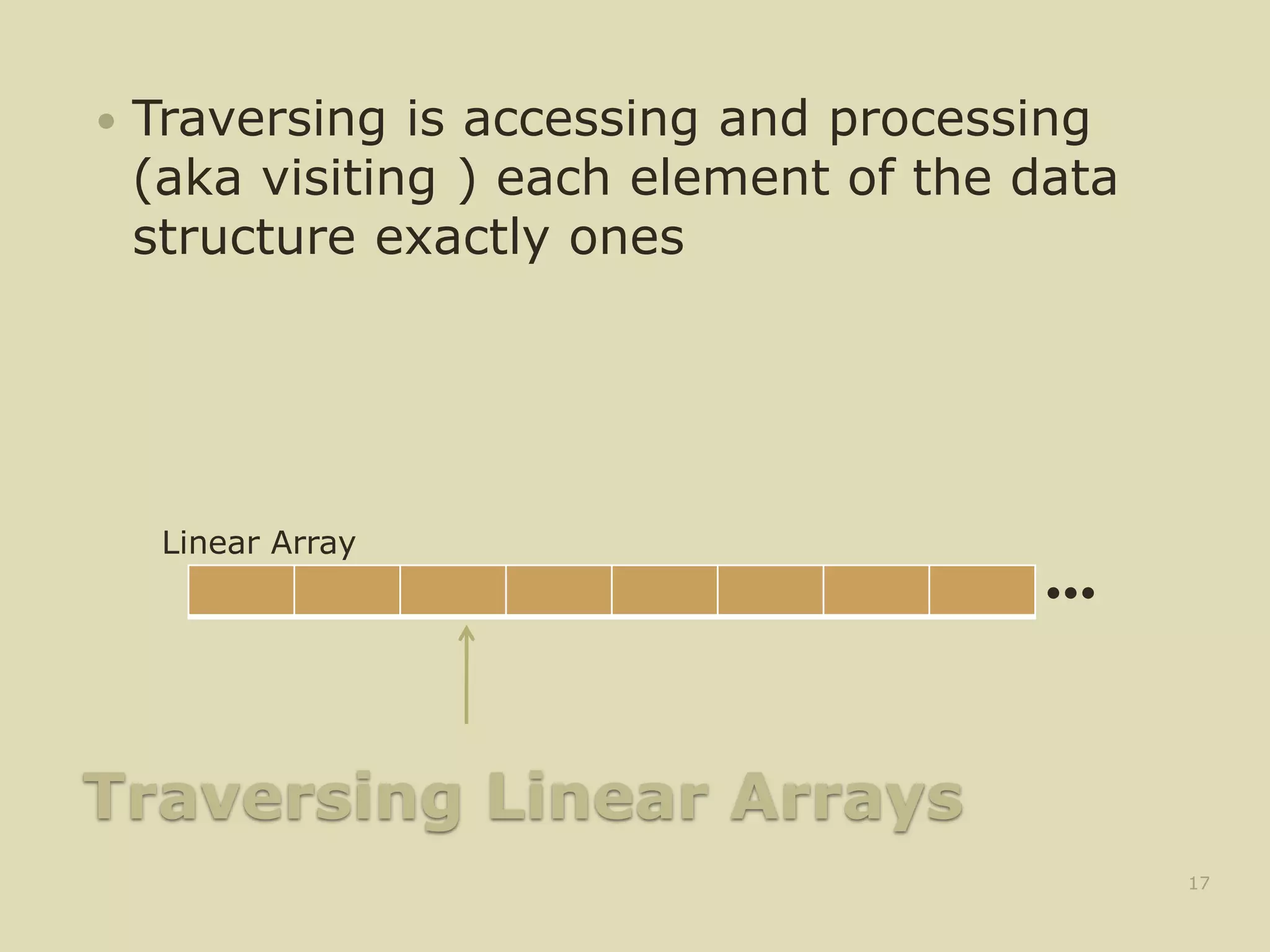
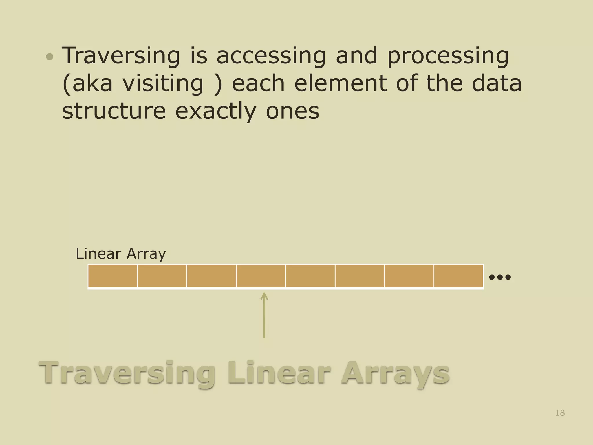
![Traversing Linear Arrays
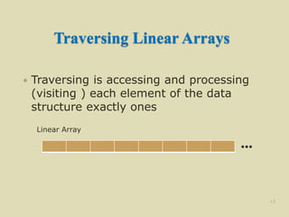
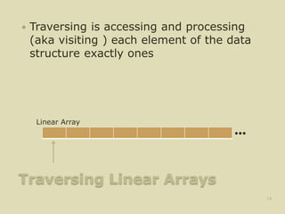
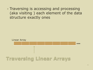
Traversing is accessing and processing
(aka visiting ) each element of the data
structure exactly ones
19
•••
Linear Array
1. Repeat for K = LB to UB
Apply PROCESS to LA[K]
[End of Loop]
2. Exit](https://image.slidesharecdn.com/arraysindatastructure-230228062337-a6c22909/85/arrays-in-data-structure-pptx-19-320.jpg)
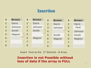
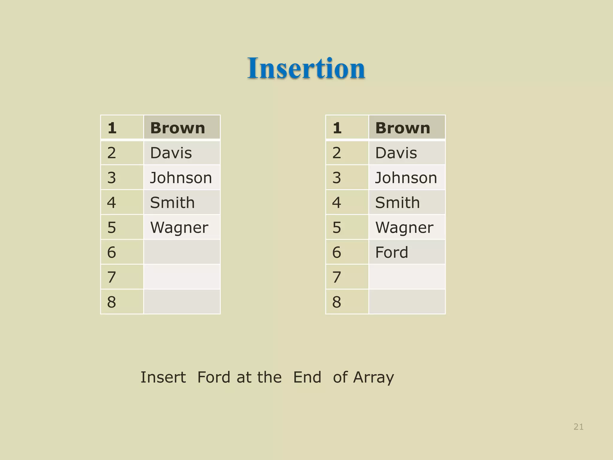
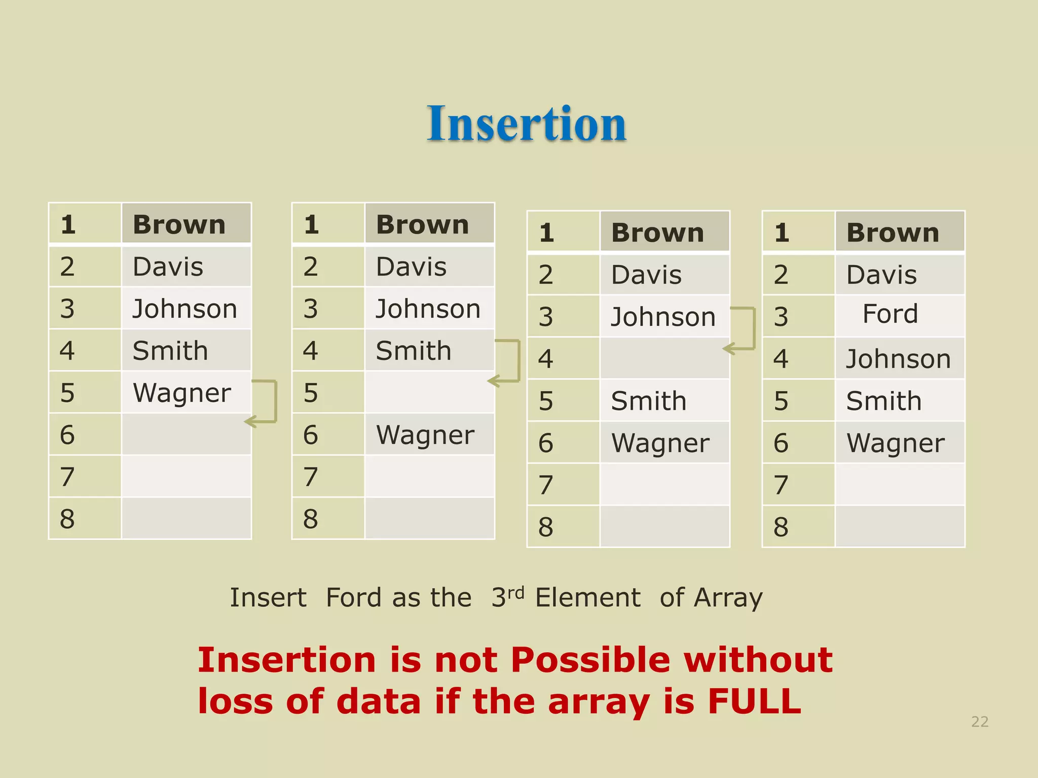
![Insertion Algorithm
INSERT (LA, N , K , ITEM) [LA is a linear
array with N elements and K is a positive integers
such that K ≤ N. This algorithm insert an element
ITEM into the Kth position in LA ]
1. [Initialize Counter] Set J := N
2. Repeat Steps 3 and 4 while J ≥ K
3. [Move the Jth element downward ] Set LA[J +
1] := LA[J]
4. [Decrease Counter] Set J := J -1
5 [Insert Element] Set LA[K] := ITEM
6. [Reset N] Set N := N +1;
7. Exit
26](https://image.slidesharecdn.com/arraysindatastructure-230228062337-a6c22909/85/arrays-in-data-structure-pptx-26-320.jpg)
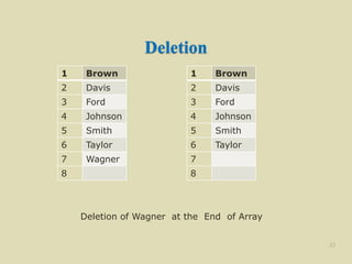
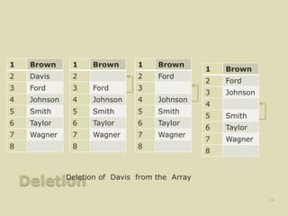
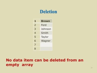
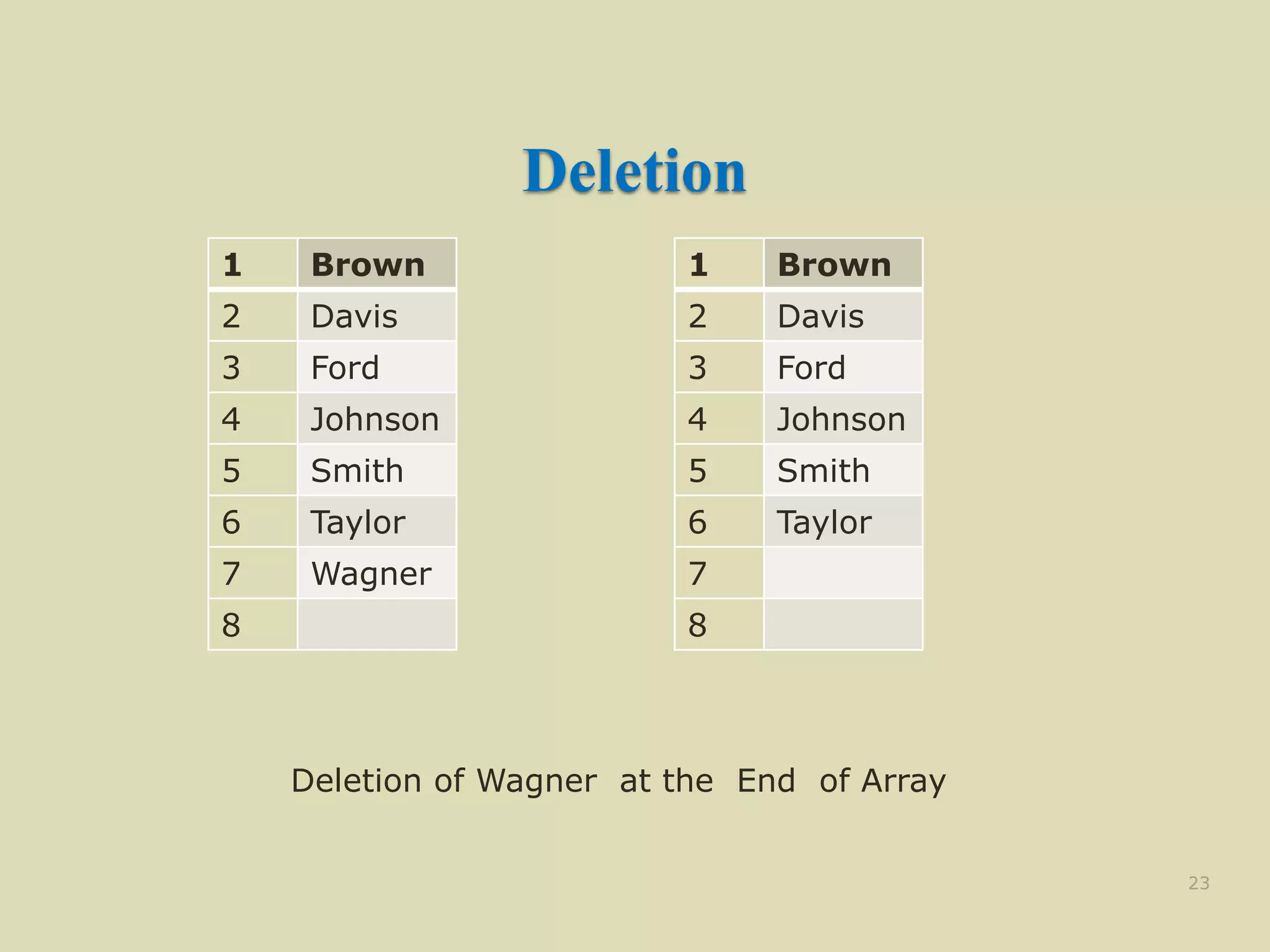
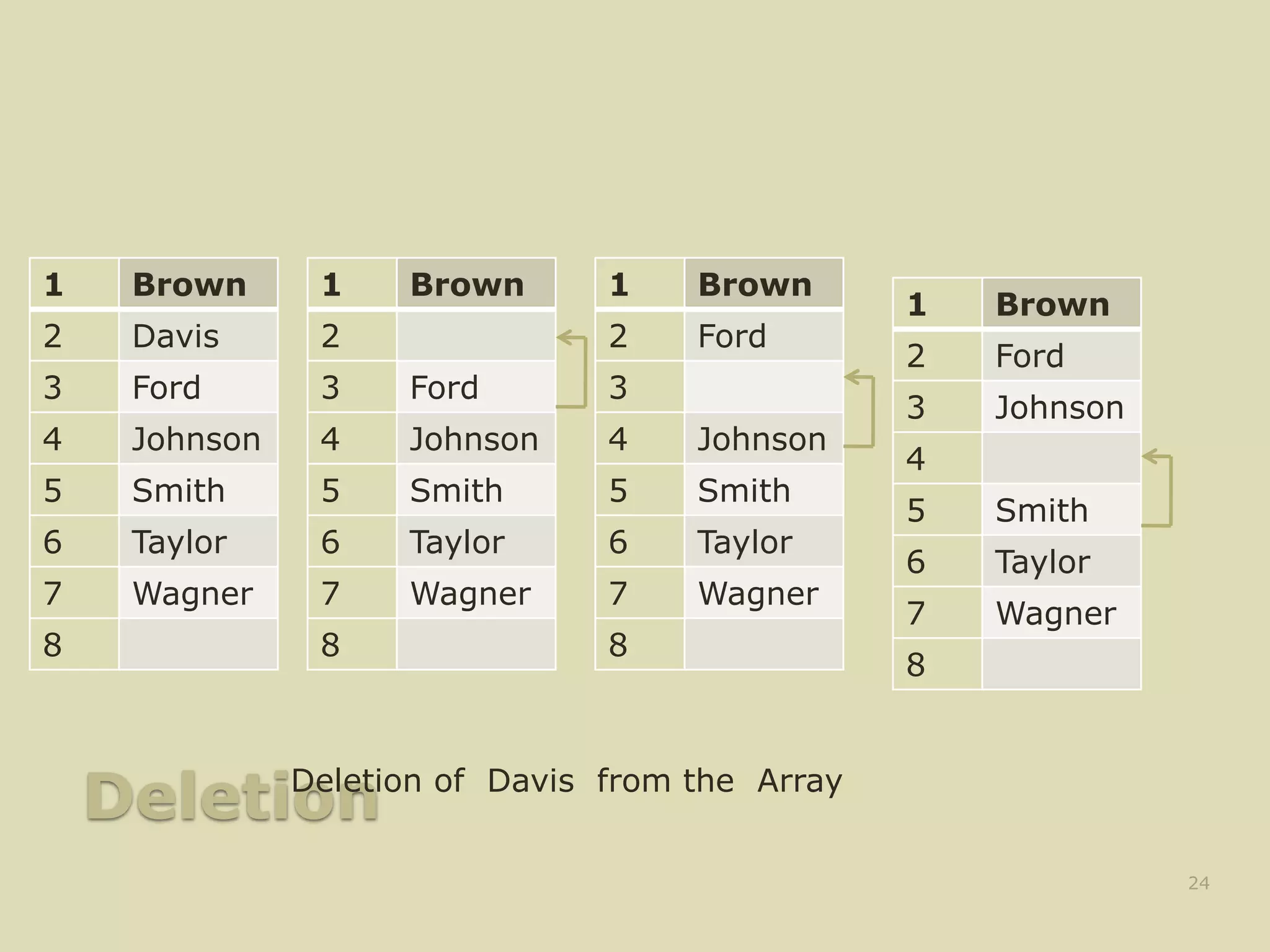
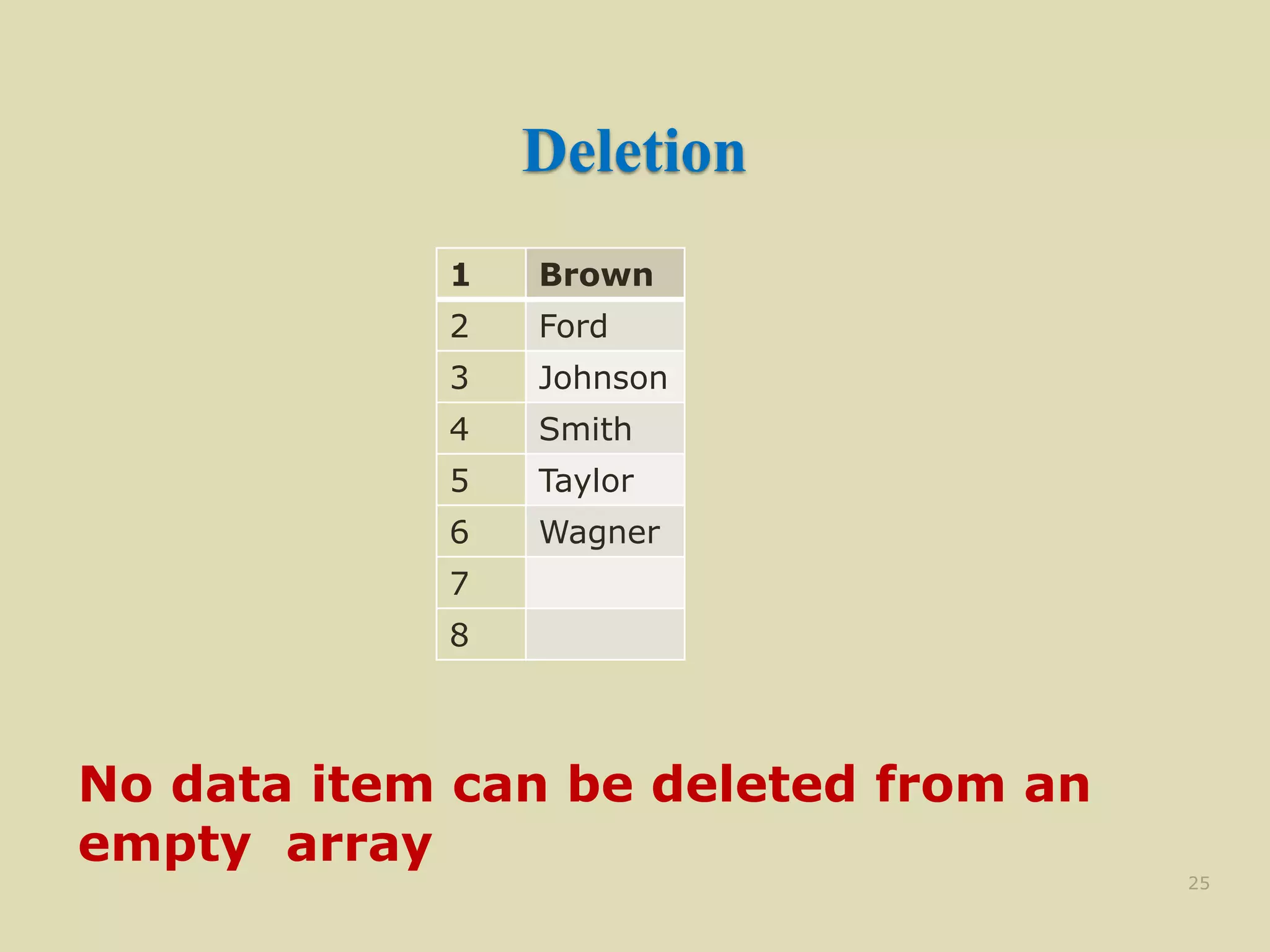
![Deletion Algorithm
DELETE (LA, N , K , ITEM) [LA is a linear
array with N elements and K is a positive integers
such that K ≤ N. This algorithm deletes Kth
element from LA ]
1. Set ITEM := LA[K]
2. Repeat for J = K to N -1:
[Move the J + 1st element upward] Set LA[J]
:= LA[J + 1]
3. [Reset the number N of elements] Set N :=
N - 1;
4. Exit
27](https://image.slidesharecdn.com/arraysindatastructure-230228062337-a6c22909/85/arrays-in-data-structure-pptx-27-320.jpg)
![Two-Dimensional Array
A Two-Dimensional m x n array A is a
collection of m . n data elements such
that each element is specified by a pair of
integer (such as J, K) called subscript with
property that
1 ≤ J ≤ m and 1 ≤ K ≤ n
The element of A with first subscript J and
second subscript K will be denoted by AJ,K
or A[J][K]
29](https://image.slidesharecdn.com/arraysindatastructure-230228062337-a6c22909/85/arrays-in-data-structure-pptx-29-320.jpg)
![2D Arrays
The elements of a 2-dimensional array a is shown as below
a[0][0] a[0][1] a[0][2]
a[0][3]
a[1][0] a[1][1] a[1][2]
a[1][3]
a[2][0] a[2][1] a[2][2]
a[2][3]](https://image.slidesharecdn.com/arraysindatastructure-230228062337-a6c22909/85/arrays-in-data-structure-pptx-30-320.jpg)
![Rows Of A 2D Array
a[0][0] a[0][1] a[0][2] a[0][3] row 0
a[1][0] a[1][1] a[1][2] a[1][3] row 1
a[2][0] a[2][1] a[2][2] a[2][3] row 2](https://image.slidesharecdn.com/arraysindatastructure-230228062337-a6c22909/85/arrays-in-data-structure-pptx-31-320.jpg)
![Columns Of A 2D Array
a[0][0] a[0][1] a[0][2] a[0][3]
a[1][0] a[1][1] a[1][2] a[1][3]
a[2][0] a[2][1] a[2][2] a[2][3]
column 0 column 1 column 2 column 3](https://image.slidesharecdn.com/arraysindatastructure-230228062337-a6c22909/85/arrays-in-data-structure-pptx-32-320.jpg)
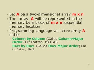
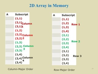
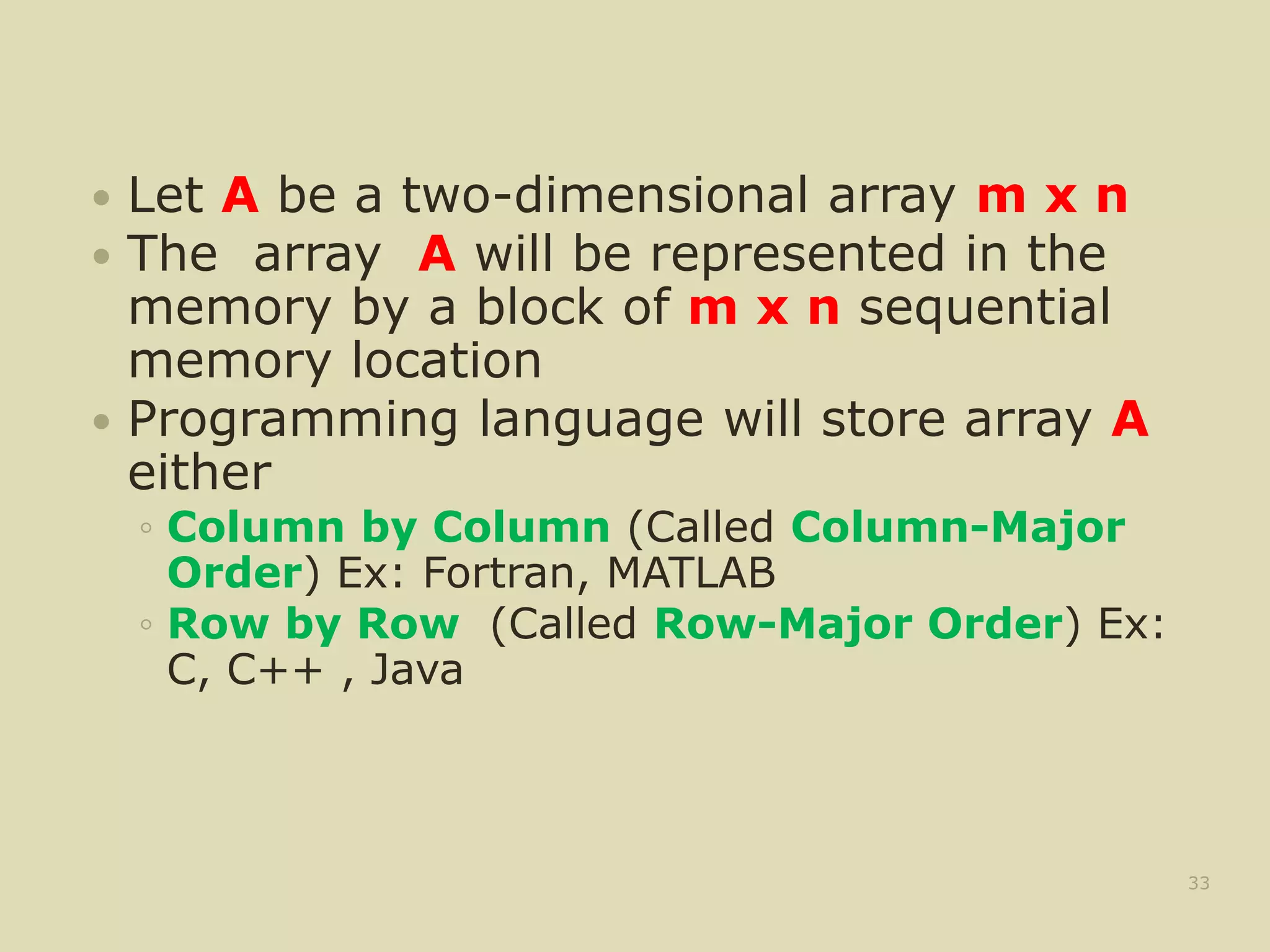
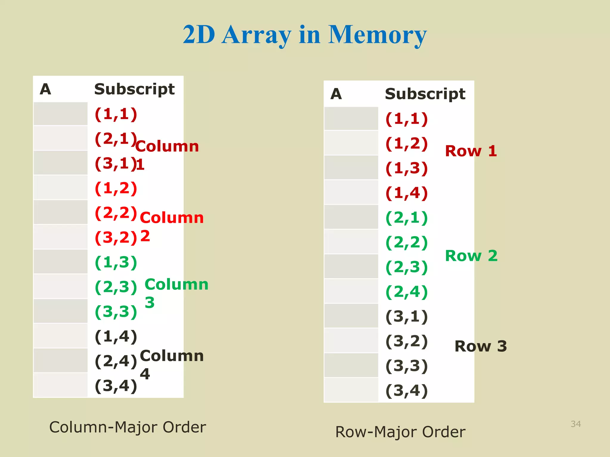
![2D Array
LOC(LA[K]) = Base(LA) + w(K -1)
LOC(A[J,K]) of A[m,n]
Column-Major Order
LOC(A[J,K]) = Base(A) + w[m(K-1) + (J-1)]
Row-Major Order
LOC(A[J,K]) = Base(A) + w[n(J-1) + (K-1)]
35](https://image.slidesharecdn.com/arraysindatastructure-230228062337-a6c22909/85/arrays-in-data-structure-pptx-35-320.jpg)
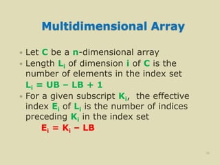
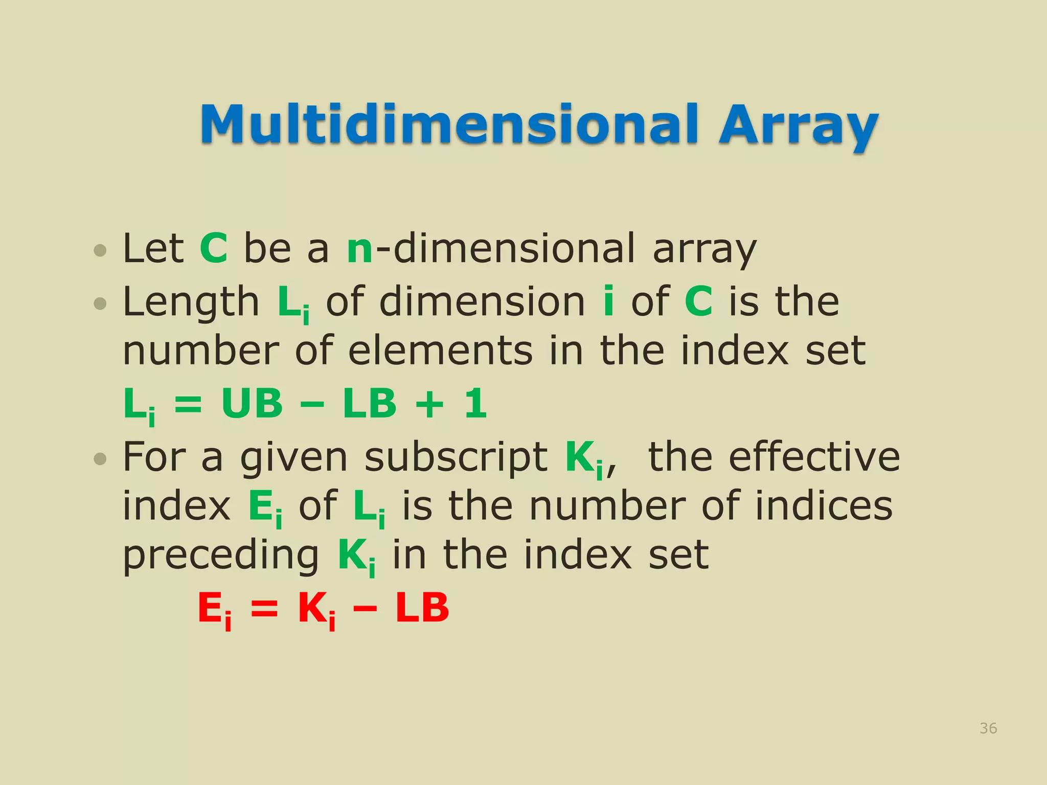
![Multidimensional Array
Address LOC(C[K1,K2, …., Kn]) of an arbitrary
element of C can be obtained as
Column-Major Order
Base( C) + w[((( … (ENLN-1 + EN-1)LN-
2) + ….. +E3)L2+E2)L1+E1]
Row-Major Order
Base( C) + w[(… ((E1L2 + E2)L3 +
E3)L4 + ….. +EN-1)LN +EN]
37](https://image.slidesharecdn.com/arraysindatastructure-230228062337-a6c22909/85/arrays-in-data-structure-pptx-37-320.jpg)

![Representation in Memory
Two basic representation in memory
◦ Have a linear relationship between the elements represented
by means of sequential memory locations [ Arrays]
◦ Have the linear relationship between the elements
represented by means of pointer or links [ Linked List]
5](https://image.slidesharecdn.com/arraysindatastructure-230228062337-a6c22909/75/arrays-in-data-structure-pptx-5-2048.jpg)
![Linear Arrays
Element of an array A may be denoted by
◦ Subscript notation A1, A2, , …. , An
◦ Parenthesis notation A(1), A(2), …. , A(n)
◦ Bracket notation A[1], A[2], ….. , A[n]
The number K in A[K] is called subscript
or an index and A[K] is called a
subscripted variable
9](https://image.slidesharecdn.com/arraysindatastructure-230228062337-a6c22909/75/arrays-in-data-structure-pptx-9-2048.jpg)
![Representation of Linear Array in Memory
Let LA be a linear array in the memory of the
computer
LOC(LA[K]) = address of the element
LA[K] of the array LA
The element of LA are stored in the
successive memory cells
Computer does not need to keep track of the
address of every element of LA, but need to
track only the address of the first element of
the array denoted by Base(LA) called the
base address of LA
11](https://image.slidesharecdn.com/arraysindatastructure-230228062337-a6c22909/75/arrays-in-data-structure-pptx-11-2048.jpg)
![Representation of Linear Array in Memory
LOC(LA[K]) = Base(LA) + w(K – lower
bound) where w is the number of words
per memory cell of the array LA
w is a size of the data type.
12](https://image.slidesharecdn.com/arraysindatastructure-230228062337-a6c22909/75/arrays-in-data-structure-pptx-12-2048.jpg)

![Traversing Linear Arrays
Traversing is accessing and processing
(aka visiting ) each element of the data
structure exactly ones
19
•••
Linear Array
1. Repeat for K = LB to UB
Apply PROCESS to LA[K]
[End of Loop]
2. Exit](https://image.slidesharecdn.com/arraysindatastructure-230228062337-a6c22909/75/arrays-in-data-structure-pptx-19-2048.jpg)
![Insertion Algorithm
INSERT (LA, N , K , ITEM) [LA is a linear
array with N elements and K is a positive integers
such that K ≤ N. This algorithm insert an element
ITEM into the Kth position in LA ]
1. [Initialize Counter] Set J := N
2. Repeat Steps 3 and 4 while J ≥ K
3. [Move the Jth element downward ] Set LA[J +
1] := LA[J]
4. [Decrease Counter] Set J := J -1
5 [Insert Element] Set LA[K] := ITEM
6. [Reset N] Set N := N +1;
7. Exit
26](https://image.slidesharecdn.com/arraysindatastructure-230228062337-a6c22909/75/arrays-in-data-structure-pptx-26-2048.jpg)
![Deletion Algorithm
DELETE (LA, N , K , ITEM) [LA is a linear
array with N elements and K is a positive integers
such that K ≤ N. This algorithm deletes Kth
element from LA ]
1. Set ITEM := LA[K]
2. Repeat for J = K to N -1:
[Move the J + 1st element upward] Set LA[J]
:= LA[J + 1]
3. [Reset the number N of elements] Set N :=
N - 1;
4. Exit
27](https://image.slidesharecdn.com/arraysindatastructure-230228062337-a6c22909/75/arrays-in-data-structure-pptx-27-2048.jpg)
![Two-Dimensional Array
A Two-Dimensional m x n array A is a
collection of m . n data elements such
that each element is specified by a pair of
integer (such as J, K) called subscript with
property that
1 ≤ J ≤ m and 1 ≤ K ≤ n
The element of A with first subscript J and
second subscript K will be denoted by AJ,K
or A[J][K]
29](https://image.slidesharecdn.com/arraysindatastructure-230228062337-a6c22909/75/arrays-in-data-structure-pptx-29-2048.jpg)
![2D Arrays
The elements of a 2-dimensional array a is shown as below
a[0][0] a[0][1] a[0][2]
a[0][3]
a[1][0] a[1][1] a[1][2]
a[1][3]
a[2][0] a[2][1] a[2][2]
a[2][3]](https://image.slidesharecdn.com/arraysindatastructure-230228062337-a6c22909/75/arrays-in-data-structure-pptx-30-2048.jpg)
![Rows Of A 2D Array
a[0][0] a[0][1] a[0][2] a[0][3] row 0
a[1][0] a[1][1] a[1][2] a[1][3] row 1
a[2][0] a[2][1] a[2][2] a[2][3] row 2](https://image.slidesharecdn.com/arraysindatastructure-230228062337-a6c22909/75/arrays-in-data-structure-pptx-31-2048.jpg)
![Columns Of A 2D Array
a[0][0] a[0][1] a[0][2] a[0][3]
a[1][0] a[1][1] a[1][2] a[1][3]
a[2][0] a[2][1] a[2][2] a[2][3]
column 0 column 1 column 2 column 3](https://image.slidesharecdn.com/arraysindatastructure-230228062337-a6c22909/75/arrays-in-data-structure-pptx-32-2048.jpg)
![2D Array
LOC(LA[K]) = Base(LA) + w(K -1)
LOC(A[J,K]) of A[m,n]
Column-Major Order
LOC(A[J,K]) = Base(A) + w[m(K-1) + (J-1)]
Row-Major Order
LOC(A[J,K]) = Base(A) + w[n(J-1) + (K-1)]
35](https://image.slidesharecdn.com/arraysindatastructure-230228062337-a6c22909/75/arrays-in-data-structure-pptx-35-2048.jpg)
![Multidimensional Array
Address LOC(C[K1,K2, …., Kn]) of an arbitrary
element of C can be obtained as
Column-Major Order
Base( C) + w[((( … (ENLN-1 + EN-1)LN-
2) + ….. +E3)L2+E2)L1+E1]
Row-Major Order
Base( C) + w[(… ((E1L2 + E2)L3 +
E3)L4 + ….. +EN-1)LN +EN]
37](https://image.slidesharecdn.com/arraysindatastructure-230228062337-a6c22909/75/arrays-in-data-structure-pptx-37-2048.jpg)


