Downloaded 1,091 times

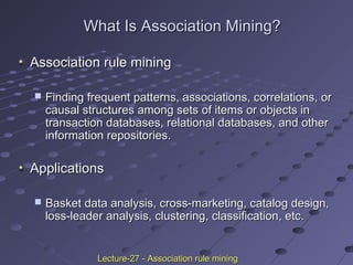
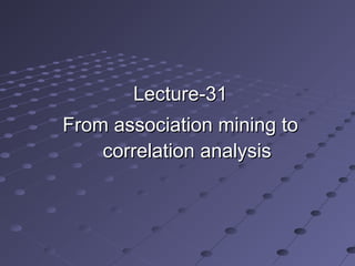
![Association MiningAssociation Mining
Rule formRule form
prediction (Boolean variables)prediction (Boolean variables) =>=>
prediction (Boolean variables) [support,prediction (Boolean variables) [support,
confidence]confidence]
Computer => antivirus_software [supportComputer => antivirus_software [support
=2%, confidence = 60%]=2%, confidence = 60%]
buys (x, “computer”)buys (x, “computer”) →→ buys (x,buys (x,
“antivirus_software”) [0.5%, 60%]“antivirus_software”) [0.5%, 60%]
Lecture-27 - Association rule miningLecture-27 - Association rule mining](https://image.slidesharecdn.com/associationrulemining-160318163143/85/Association-rule-mining-3-320.jpg)
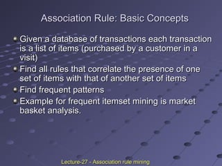
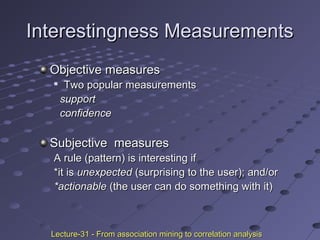
![Association Rule Mining: A Road MapAssociation Rule Mining: A Road Map
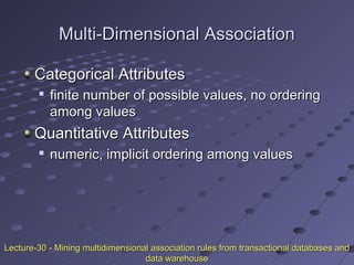
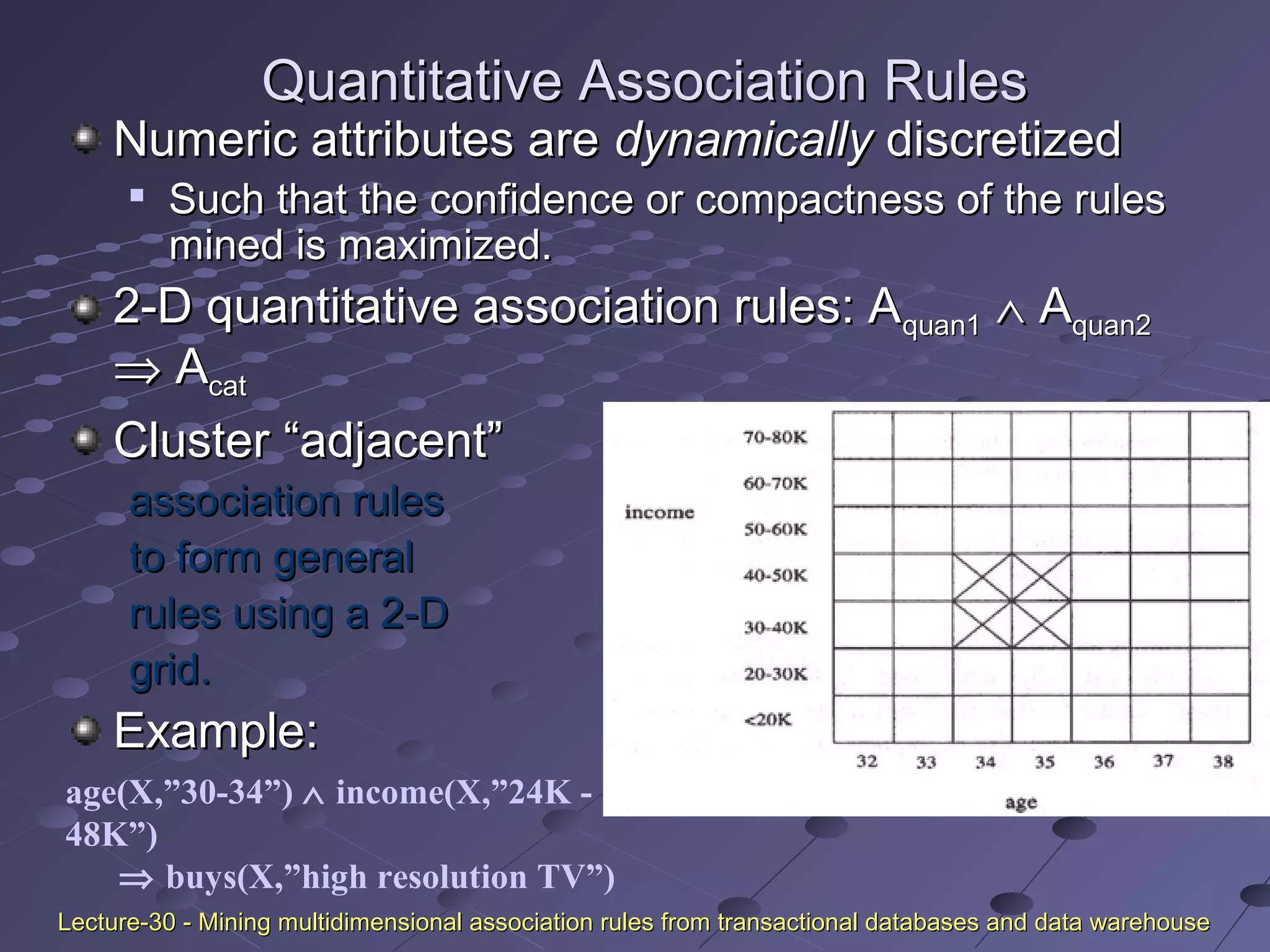
Boolean vs. quantitative associationsBoolean vs. quantitative associations
- Based on the types of values handled- Based on the types of values handled
buys(x, “SQLServer”) ^ buys(x, “DMBook”)buys(x, “SQLServer”) ^ buys(x, “DMBook”) =>=> buys(x,buys(x,
“DBMiner”) [0.2%, 60%]“DBMiner”) [0.2%, 60%]
age(x, “30..39”) ^ income(x, “42..48K”)age(x, “30..39”) ^ income(x, “42..48K”) =>=> buys(x, “PC”)buys(x, “PC”)
[1%, 75%][1%, 75%]
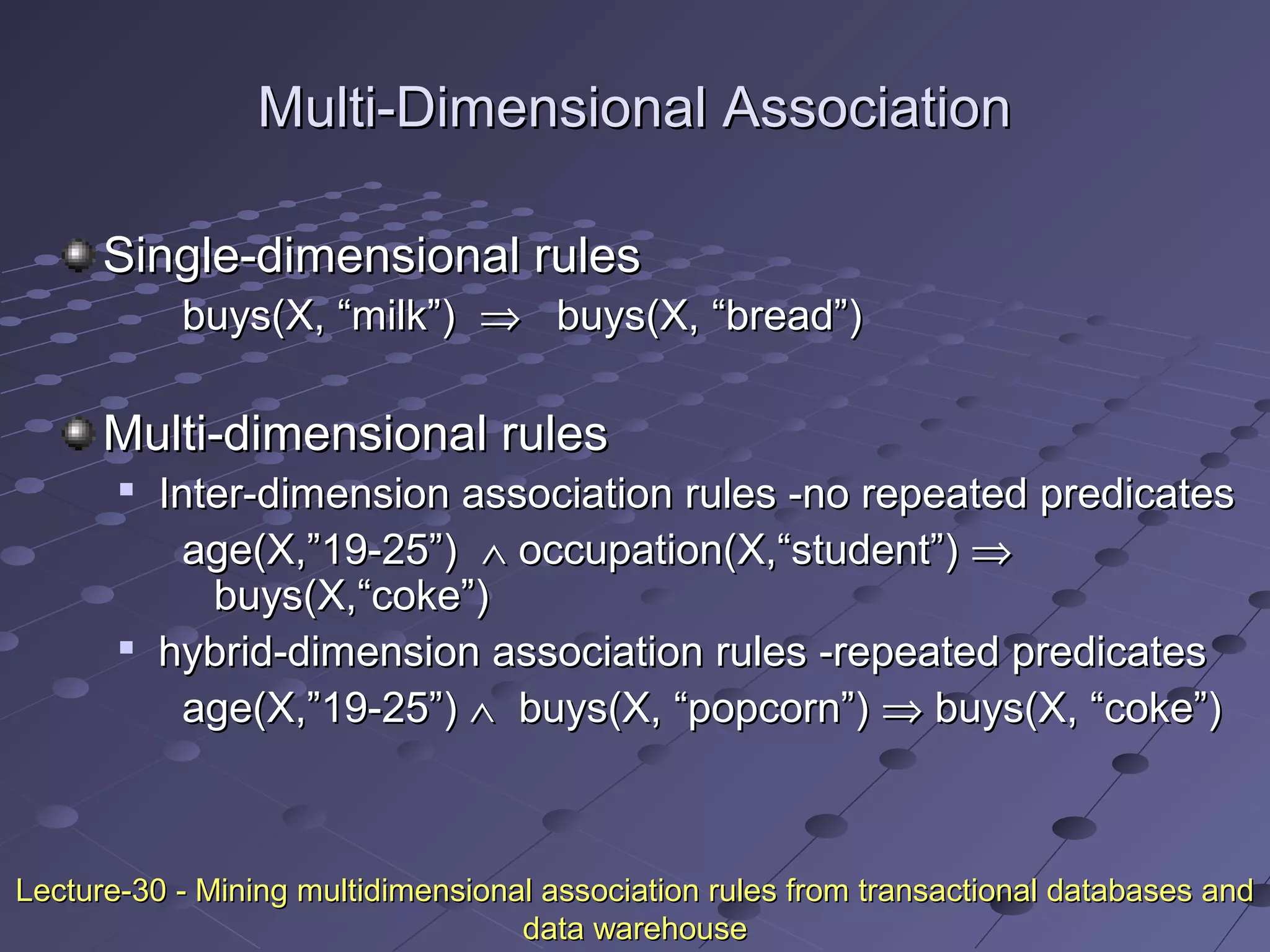
Single dimension vs. multiple dimensionalSingle dimension vs. multiple dimensional
associationsassociations
Single level vs. multiple-level analysisSingle level vs. multiple-level analysis
Lecture-27 - Association rule miningLecture-27 - Association rule mining](https://image.slidesharecdn.com/associationrulemining-160318163143/85/Association-rule-mining-8-320.jpg)

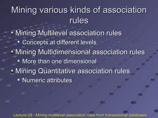
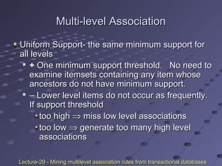
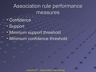
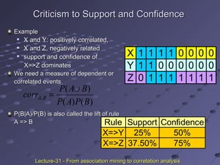
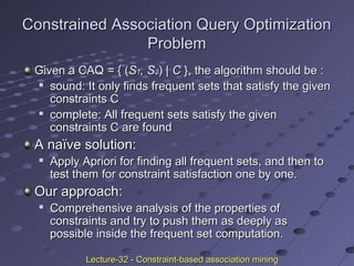
![Uniform SupportUniform Support
Multi-level mining with uniform supportMulti-level mining with uniform support
Milk
[support = 10%]
2% Milk
[support = 6%]
Skim Milk
[support = 4%]
Level 1
min_sup = 5%
Level 2
min_sup = 5%
Back
Lecture-29 - Mining multilevel association rules from transactional databasesLecture-29 - Mining multilevel association rules from transactional databases](https://image.slidesharecdn.com/associationrulemining-160318163143/85/Association-rule-mining-27-320.jpg)
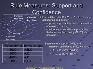
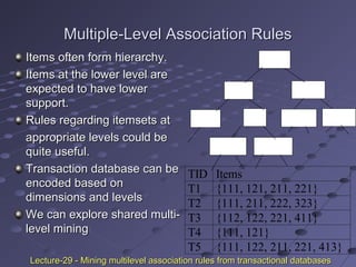
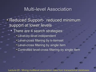
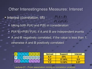
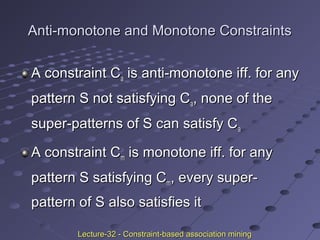
![Reduced SupportReduced Support
Multi-level mining with reduced supportMulti-level mining with reduced support
2% Milk
[support = 6%]
Skim Milk
[support = 4%]
Level 1
min_sup = 5%
Level 2
min_sup = 3%
Milk
[support = 10%]
Lecture-29 - Mining multilevel association rules from transactional databasesLecture-29 - Mining multilevel association rules from transactional databases](https://image.slidesharecdn.com/associationrulemining-160318163143/85/Association-rule-mining-28-320.jpg)
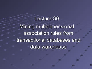
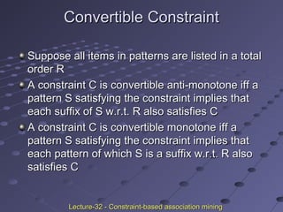
![Multi-level Association: RedundancyMulti-level Association: Redundancy
FilteringFiltering
Some rules may be redundant due to “ancestor”Some rules may be redundant due to “ancestor”
relationships between items.relationships between items.
ExampleExample
milkmilk ⇒⇒ wheat breadwheat bread [support = 8%, confidence = 70%][support = 8%, confidence = 70%]
2% milk2% milk ⇒⇒ wheat breadwheat bread [support = 2%, confidence = 72%][support = 2%, confidence = 72%]
We say the first rule is an ancestor of the secondWe say the first rule is an ancestor of the second
rule.rule.
A rule is redundant if its support is close to theA rule is redundant if its support is close to the
“expected” value, based on the rule’s ancestor.“expected” value, based on the rule’s ancestor.
Lecture-29 - Mining multilevel association rules from transactional databasesLecture-29 - Mining multilevel association rules from transactional databases](https://image.slidesharecdn.com/associationrulemining-160318163143/85/Association-rule-mining-29-320.jpg)
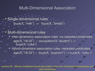
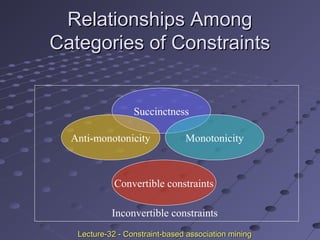
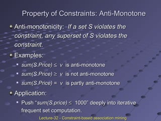
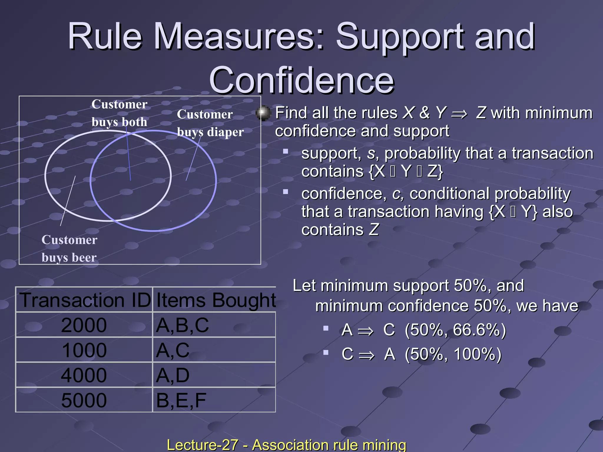
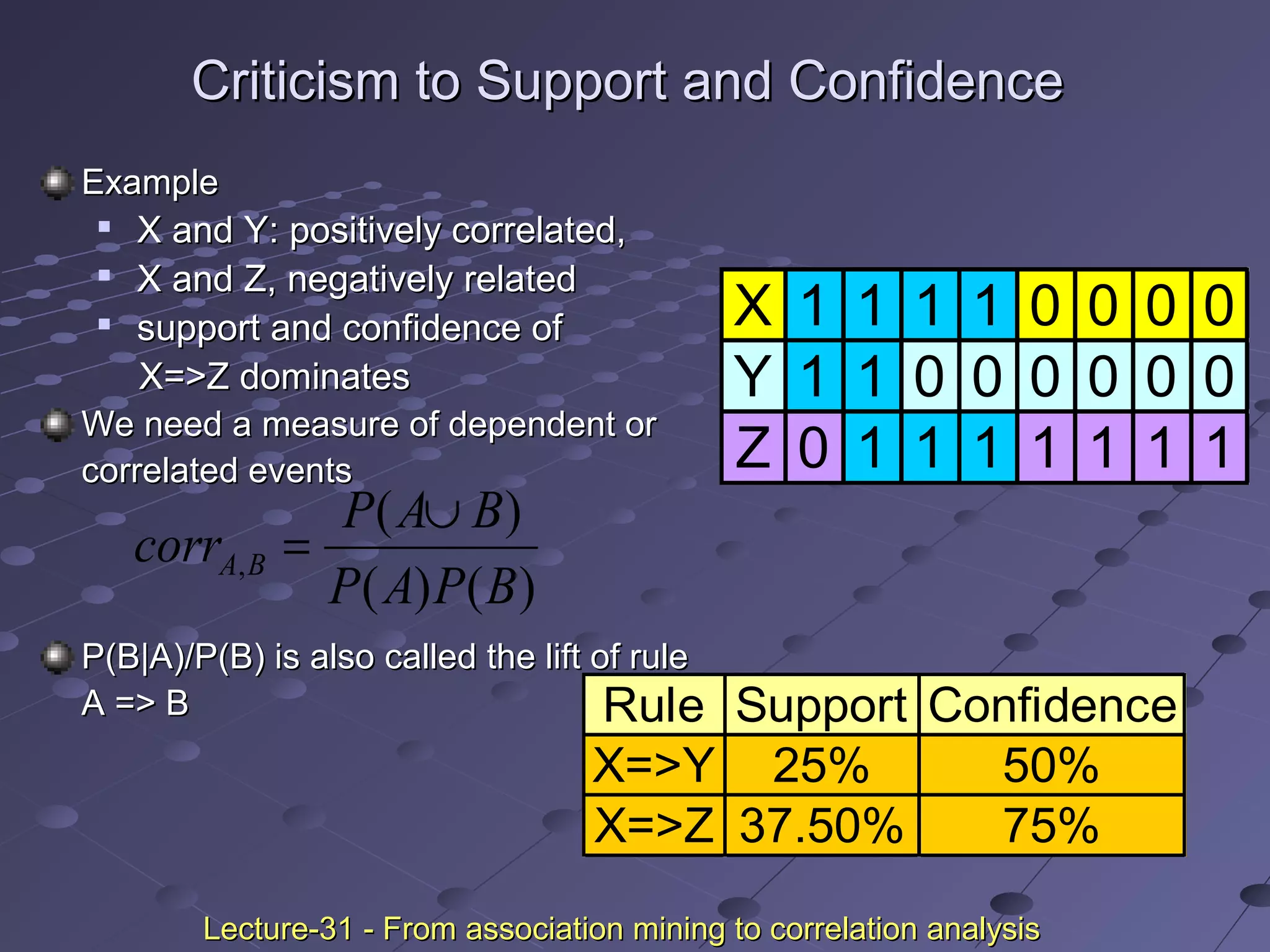
![Criticism to Support and ConfidenceCriticism to Support and Confidence
ExampleExample
Among 5000 studentsAmong 5000 students
3000 play basketball3000 play basketball
3750 eat cereal3750 eat cereal
2000 both play basket ball and eat cereal2000 both play basket ball and eat cereal
play basketballplay basketball ⇒⇒ eat cerealeat cereal [40%, 66.7%] is misleading[40%, 66.7%] is misleading
because the overall percentage of students eating cereal is 75%because the overall percentage of students eating cereal is 75%
which is higher than 66.7%.which is higher than 66.7%.
play basketballplay basketball ⇒⇒ not eat cerealnot eat cereal [20%, 33.3%] is far more[20%, 33.3%] is far more
accurate, although with lower support and confidenceaccurate, although with lower support and confidence
basketball not basketball sum(row)
cereal 2000 1750 3750
not cereal 1000 250 1250
sum(col.) 3000 2000 5000
Lecture-31 - From association mining to correlation analysisLecture-31 - From association mining to correlation analysis](https://image.slidesharecdn.com/associationrulemining-160318163143/85/Association-rule-mining-38-320.jpg)


![Association MiningAssociation Mining
Rule formRule form
prediction (Boolean variables)prediction (Boolean variables) =>=>
prediction (Boolean variables) [support,prediction (Boolean variables) [support,
confidence]confidence]
Computer => antivirus_software [supportComputer => antivirus_software [support
=2%, confidence = 60%]=2%, confidence = 60%]
buys (x, “computer”)buys (x, “computer”) →→ buys (x,buys (x,
“antivirus_software”) [0.5%, 60%]“antivirus_software”) [0.5%, 60%]
Lecture-27 - Association rule miningLecture-27 - Association rule mining](https://image.slidesharecdn.com/associationrulemining-160318163143/75/Association-rule-mining-3-2048.jpg)
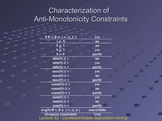
![Association Rule Mining: A Road MapAssociation Rule Mining: A Road Map
Boolean vs. quantitative associationsBoolean vs. quantitative associations
- Based on the types of values handled- Based on the types of values handled
buys(x, “SQLServer”) ^ buys(x, “DMBook”)buys(x, “SQLServer”) ^ buys(x, “DMBook”) =>=> buys(x,buys(x,
“DBMiner”) [0.2%, 60%]“DBMiner”) [0.2%, 60%]
age(x, “30..39”) ^ income(x, “42..48K”)age(x, “30..39”) ^ income(x, “42..48K”) =>=> buys(x, “PC”)buys(x, “PC”)
[1%, 75%][1%, 75%]
Single dimension vs. multiple dimensionalSingle dimension vs. multiple dimensional
associationsassociations
Single level vs. multiple-level analysisSingle level vs. multiple-level analysis
Lecture-27 - Association rule miningLecture-27 - Association rule mining](https://image.slidesharecdn.com/associationrulemining-160318163143/75/Association-rule-mining-8-2048.jpg)

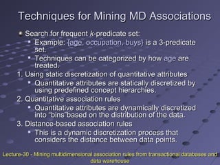
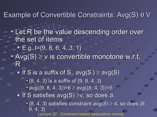
![Uniform SupportUniform Support
Multi-level mining with uniform supportMulti-level mining with uniform support
Milk
[support = 10%]
2% Milk
[support = 6%]
Skim Milk
[support = 4%]
Level 1
min_sup = 5%
Level 2
min_sup = 5%
Back
Lecture-29 - Mining multilevel association rules from transactional databasesLecture-29 - Mining multilevel association rules from transactional databases](https://image.slidesharecdn.com/associationrulemining-160318163143/75/Association-rule-mining-27-2048.jpg)
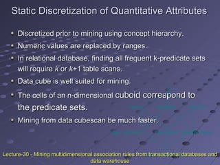
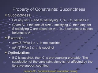
![Reduced SupportReduced Support
Multi-level mining with reduced supportMulti-level mining with reduced support
2% Milk
[support = 6%]
Skim Milk
[support = 4%]
Level 1
min_sup = 5%
Level 2
min_sup = 3%
Milk
[support = 10%]
Lecture-29 - Mining multilevel association rules from transactional databasesLecture-29 - Mining multilevel association rules from transactional databases](https://image.slidesharecdn.com/associationrulemining-160318163143/75/Association-rule-mining-28-2048.jpg)
![Multi-level Association: RedundancyMulti-level Association: Redundancy
FilteringFiltering
Some rules may be redundant due to “ancestor”Some rules may be redundant due to “ancestor”
relationships between items.relationships between items.
ExampleExample
milkmilk ⇒⇒ wheat breadwheat bread [support = 8%, confidence = 70%][support = 8%, confidence = 70%]
2% milk2% milk ⇒⇒ wheat breadwheat bread [support = 2%, confidence = 72%][support = 2%, confidence = 72%]
We say the first rule is an ancestor of the secondWe say the first rule is an ancestor of the second
rule.rule.
A rule is redundant if its support is close to theA rule is redundant if its support is close to the
“expected” value, based on the rule’s ancestor.“expected” value, based on the rule’s ancestor.
Lecture-29 - Mining multilevel association rules from transactional databasesLecture-29 - Mining multilevel association rules from transactional databases](https://image.slidesharecdn.com/associationrulemining-160318163143/75/Association-rule-mining-29-2048.jpg)
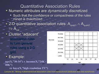
![Criticism to Support and ConfidenceCriticism to Support and Confidence
ExampleExample
Among 5000 studentsAmong 5000 students
3000 play basketball3000 play basketball
3750 eat cereal3750 eat cereal
2000 both play basket ball and eat cereal2000 both play basket ball and eat cereal
play basketballplay basketball ⇒⇒ eat cerealeat cereal [40%, 66.7%] is misleading[40%, 66.7%] is misleading
because the overall percentage of students eating cereal is 75%because the overall percentage of students eating cereal is 75%
which is higher than 66.7%.which is higher than 66.7%.
play basketballplay basketball ⇒⇒ not eat cerealnot eat cereal [20%, 33.3%] is far more[20%, 33.3%] is far more
accurate, although with lower support and confidenceaccurate, although with lower support and confidence
basketball not basketball sum(row)
cereal 2000 1750 3750
not cereal 1000 250 1250
sum(col.) 3000 2000 5000
Lecture-31 - From association mining to correlation analysisLecture-31 - From association mining to correlation analysis](https://image.slidesharecdn.com/associationrulemining-160318163143/75/Association-rule-mining-38-2048.jpg)
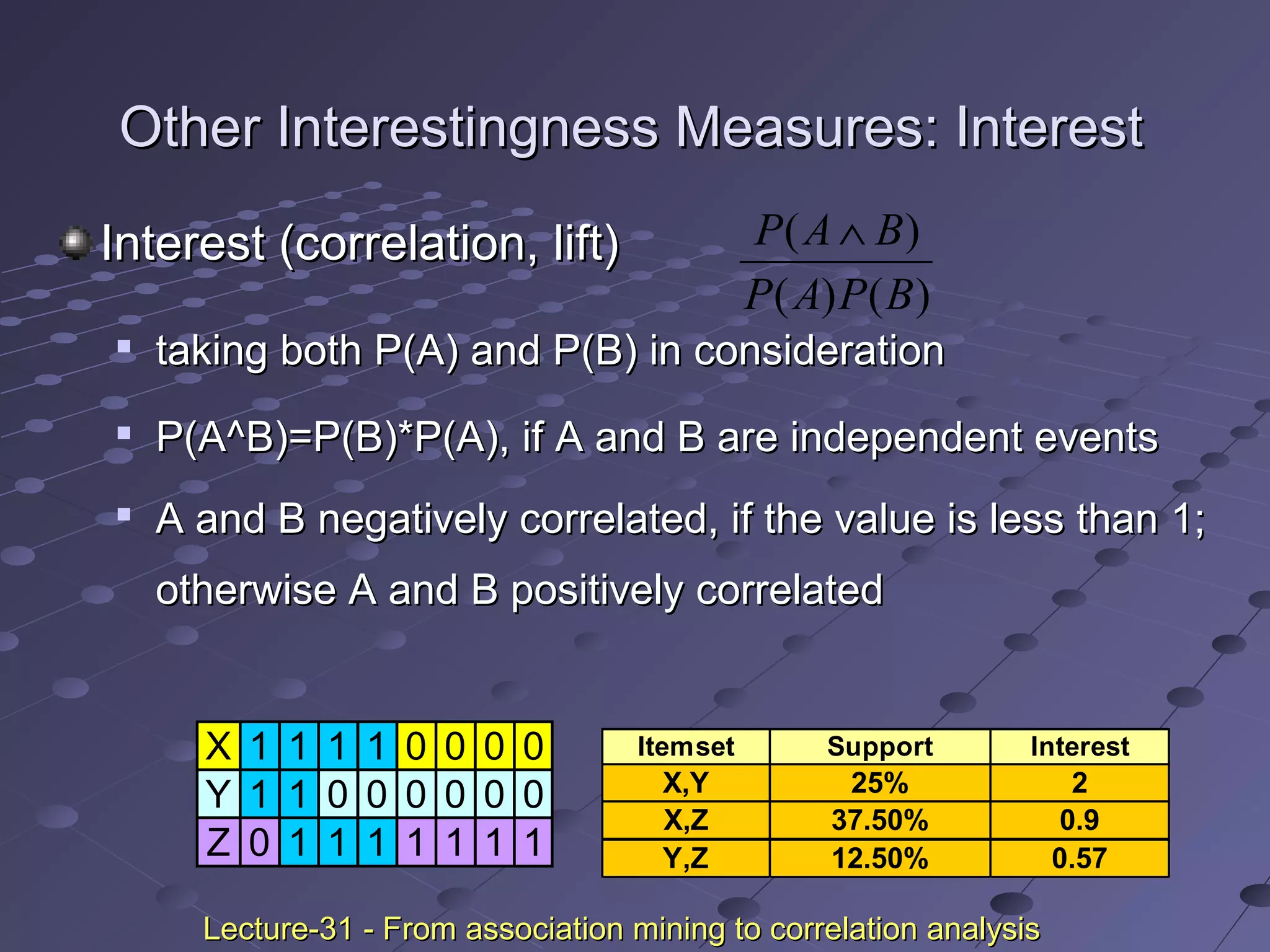


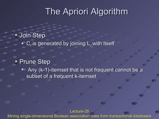
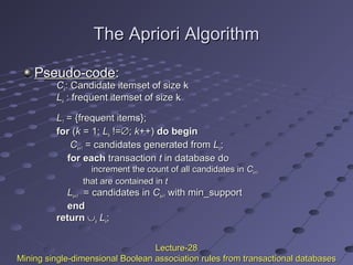
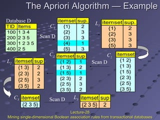
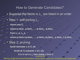
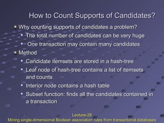
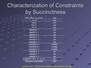
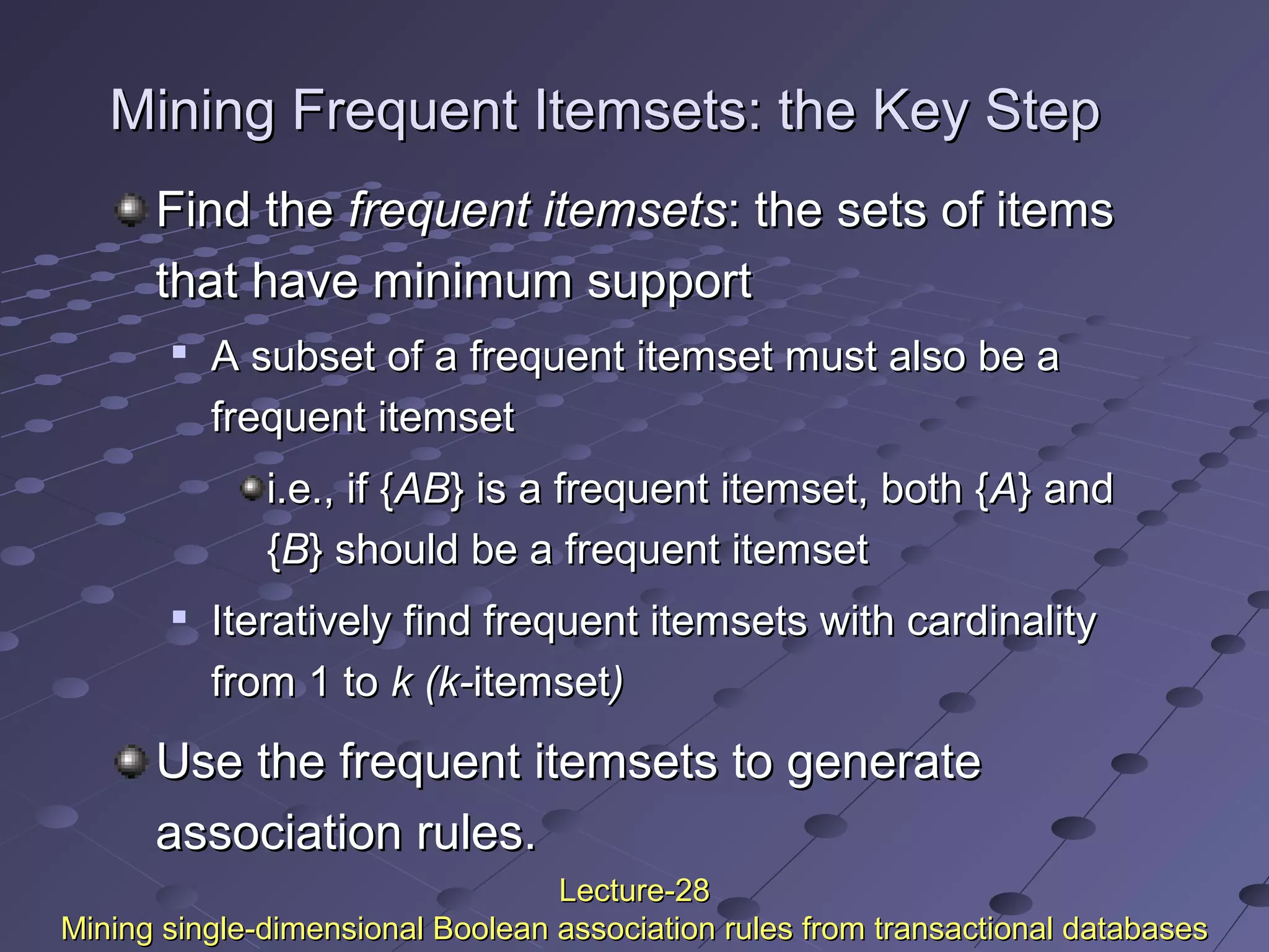
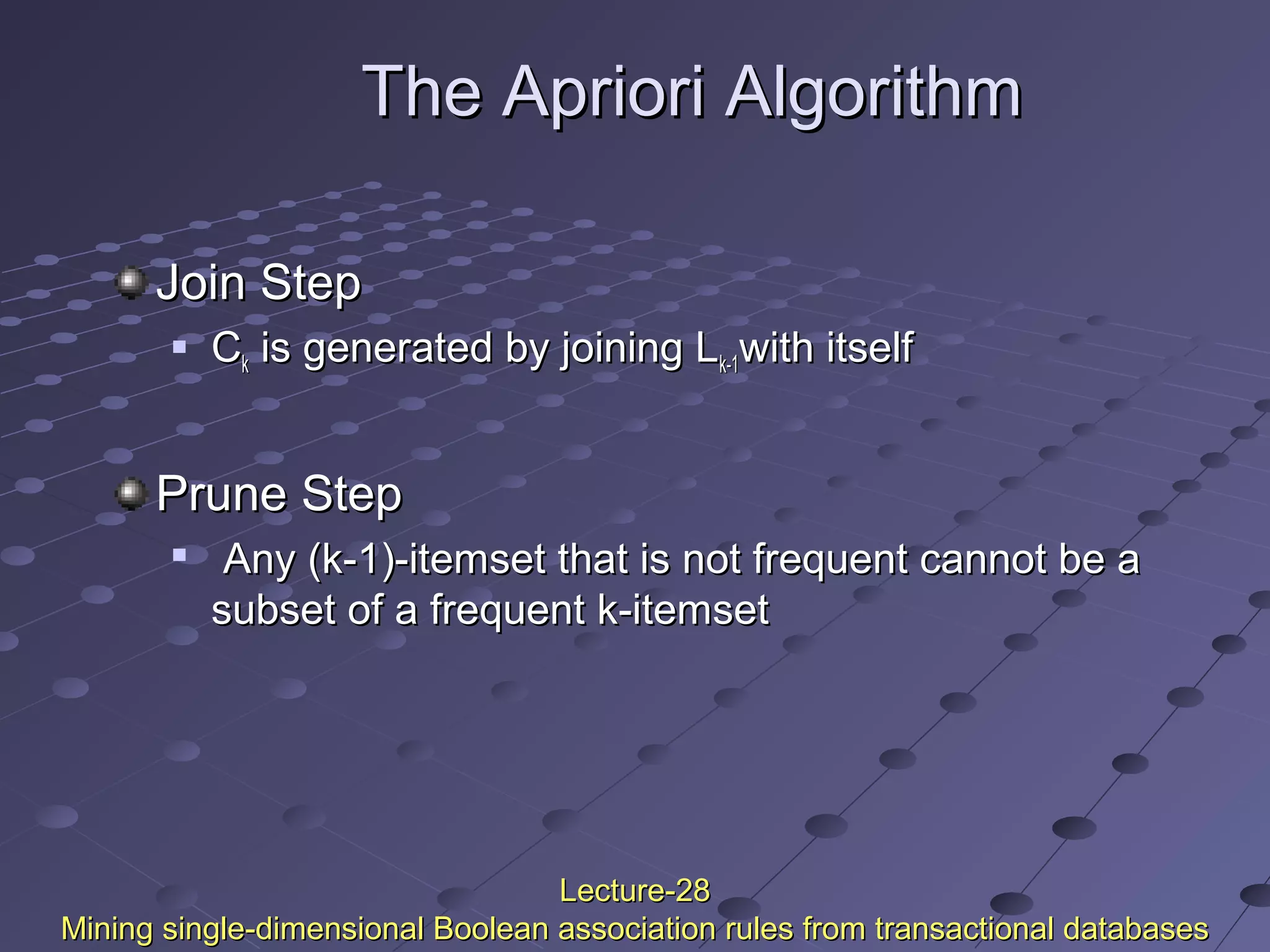
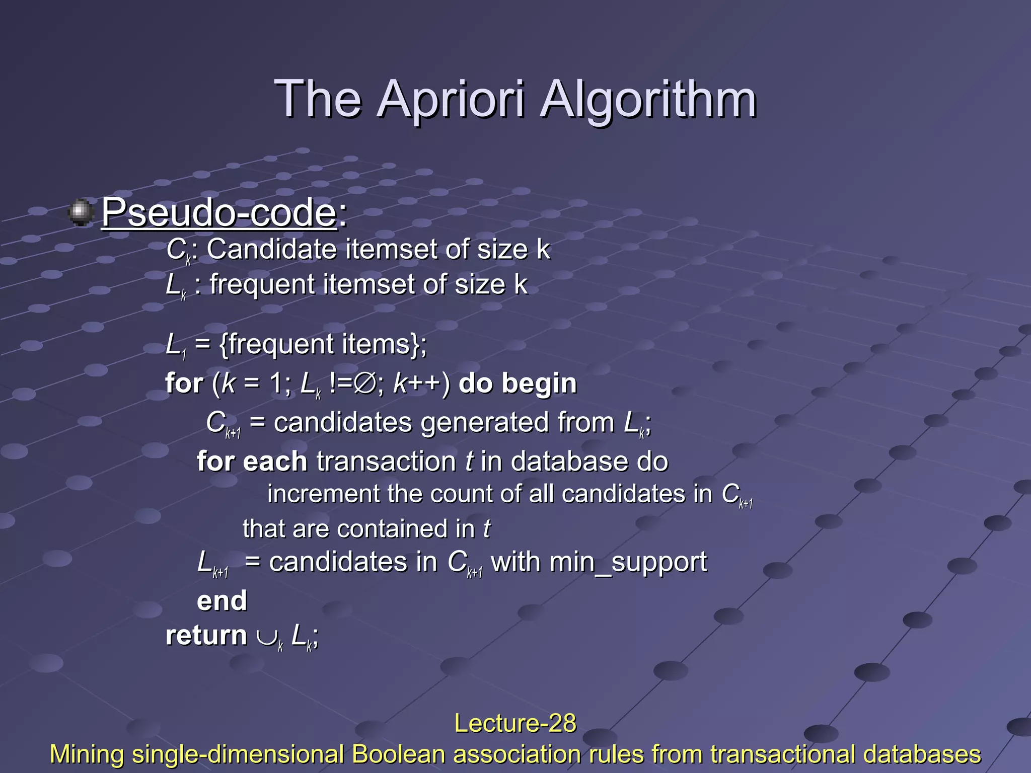
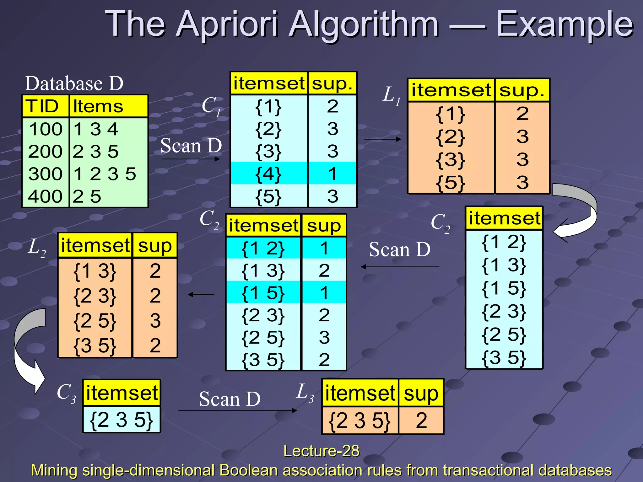
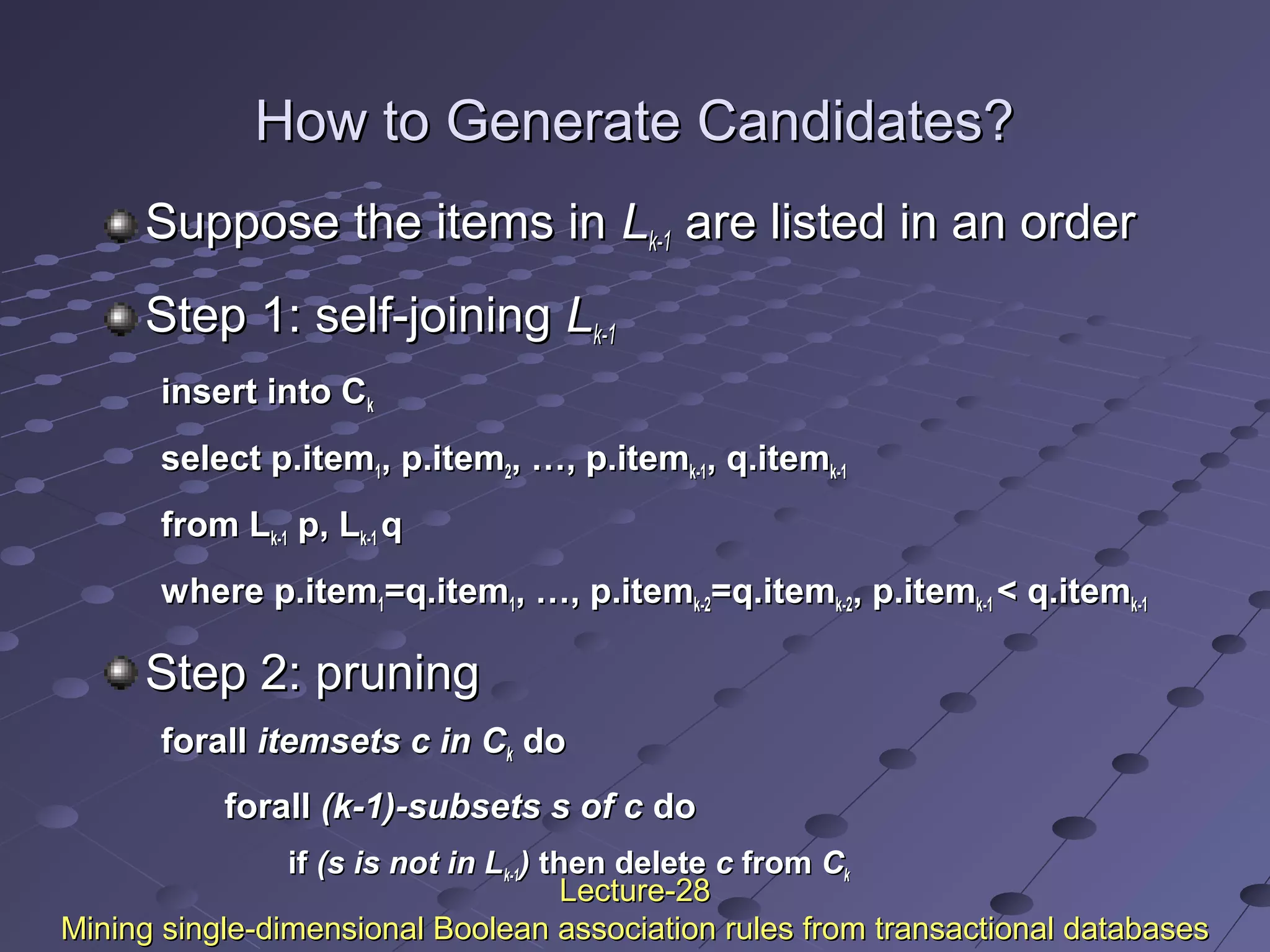
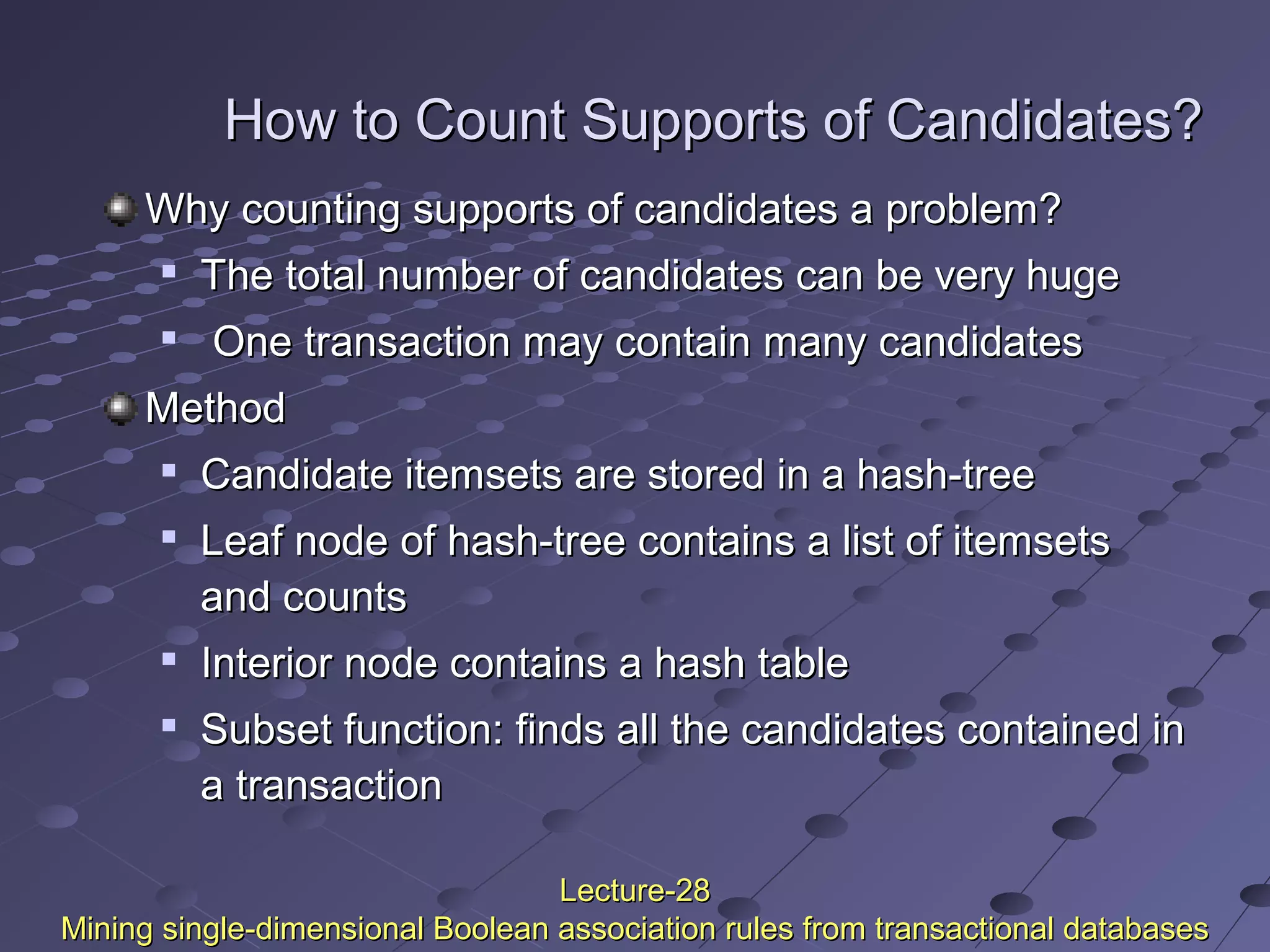
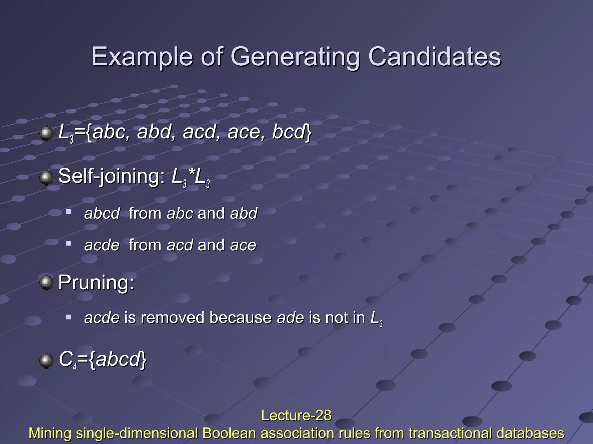
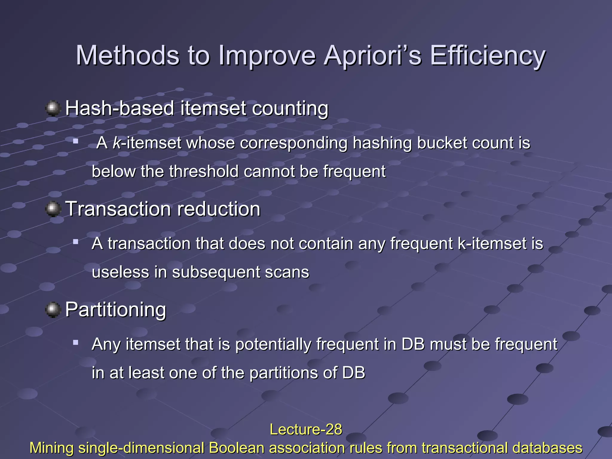
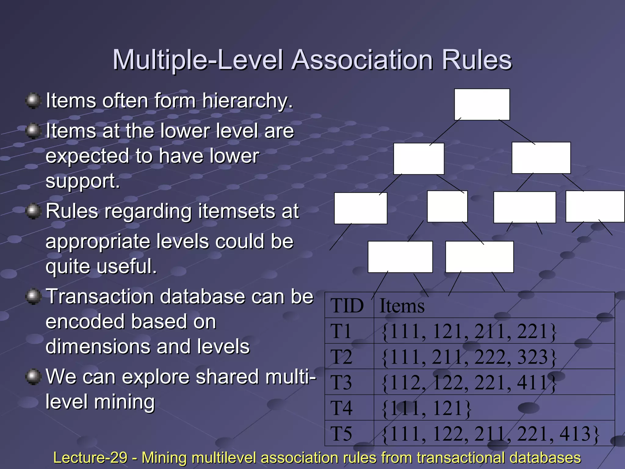
This document discusses association rule mining. Association rule mining finds frequent patterns, associations, correlations, or causal structures among items in transaction databases. The Apriori algorithm is commonly used to find frequent itemsets and generate association rules. It works by iteratively joining frequent itemsets from the previous pass to generate candidates, and then pruning the candidates that have infrequent subsets. Various techniques can improve the efficiency of Apriori, such as hashing to count itemsets and pruning transactions that don't contain frequent itemsets. Alternative approaches like FP-growth compress the database into a tree structure to avoid costly scans and candidate generation. The document also discusses mining multilevel, multidimensional, and quantitative association rules.


