Downloaded 38 times


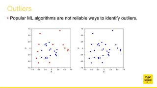
![Outliers
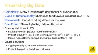
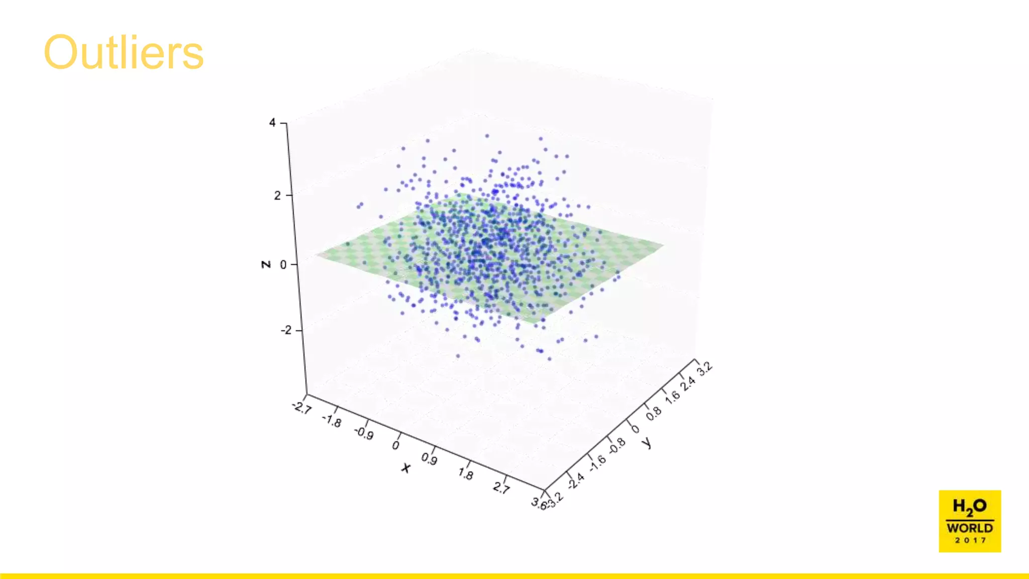
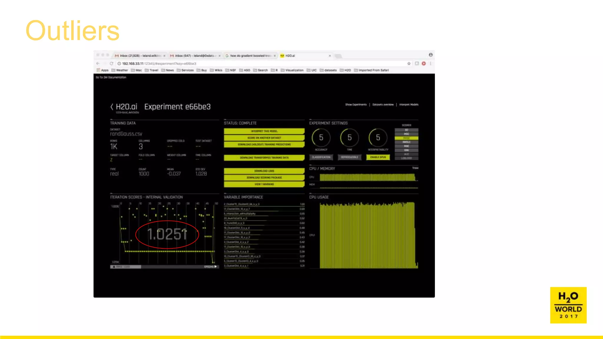
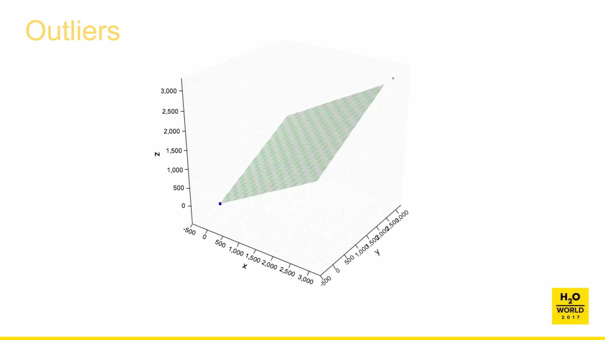
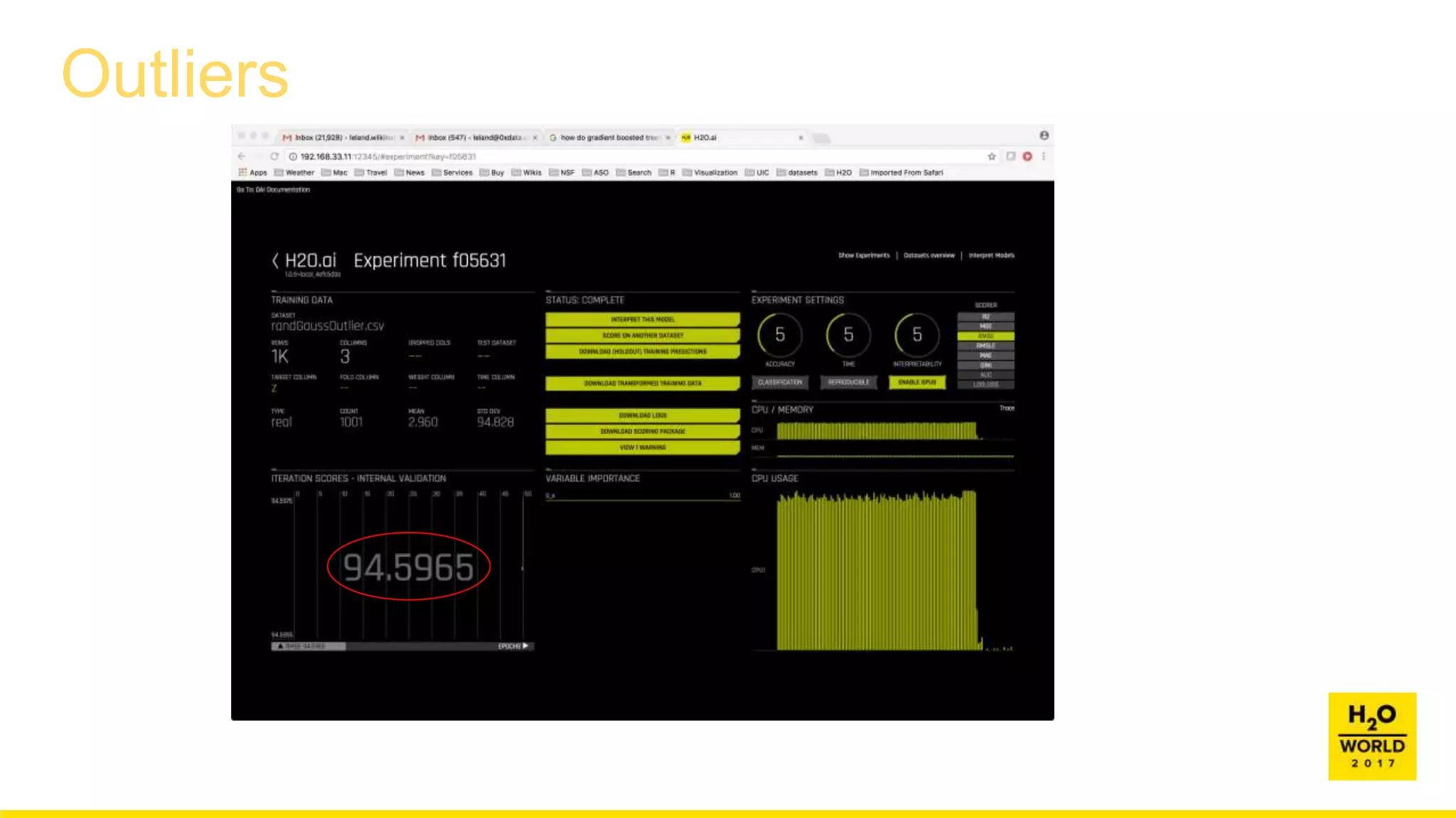
1. Map categorical variables to continuous values (SVD).
2. If p large, use random projections to reduce dimensionality.
3. Normalize columns on [0, 1]
4. If n large, aggregate
• If p = 2, you could use gridding or hex binning
• But general solution is based on Hartigan’s Leader algorithm
5. Compute nearest neighbor distances between points.
6. Fit exponential distribution to largest distances.
7. Reject points in upper tail of this distribution.](https://image.slidesharecdn.com/wilkinson-171208083154/85/Automatic-Visualization-Leland-Wilkinson-Chief-Scientist-H2O-ai-12-320.jpg)


![Outliers
1. Map categorical variables to continuous values (SVD).
2. If p large, use random projections to reduce dimensionality.
3. Normalize columns on [0, 1]
4. If n large, aggregate
• If p = 2, you could use gridding or hex binning
• But general solution is based on Hartigan’s Leader algorithm
5. Compute nearest neighbor distances between points.
6. Fit exponential distribution to largest distances.
7. Reject points in upper tail of this distribution.](https://image.slidesharecdn.com/wilkinson-171208083154/75/Automatic-Visualization-Leland-Wilkinson-Chief-Scientist-H2O-ai-12-2048.jpg)
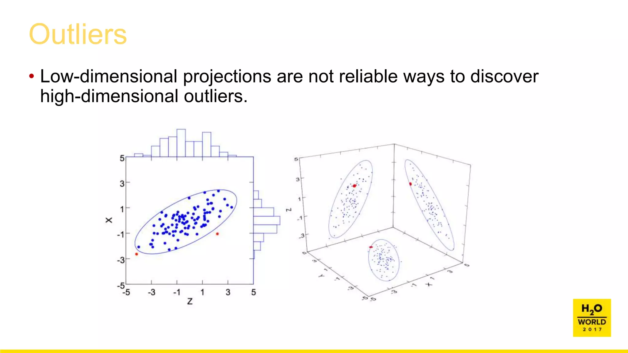
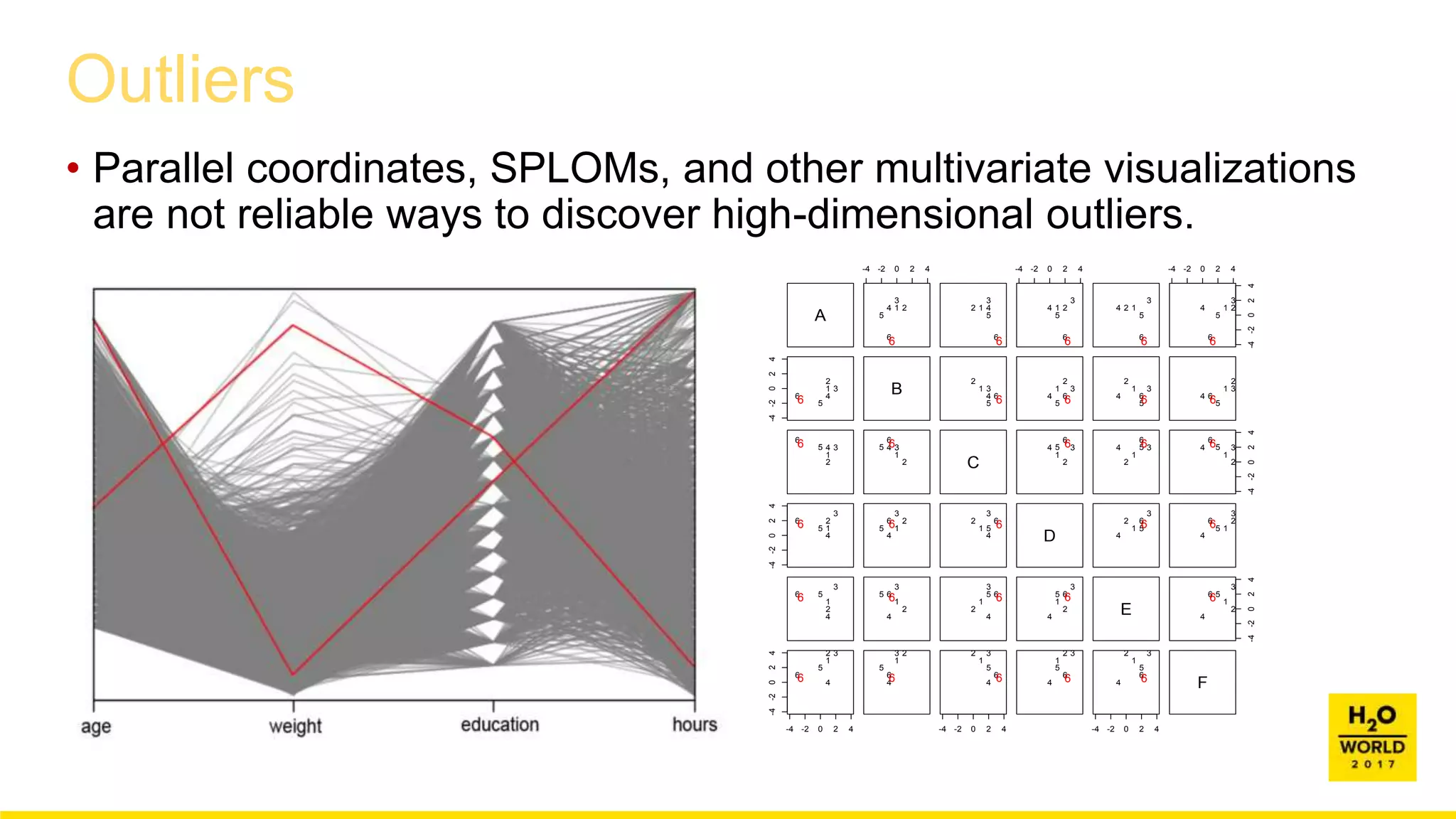
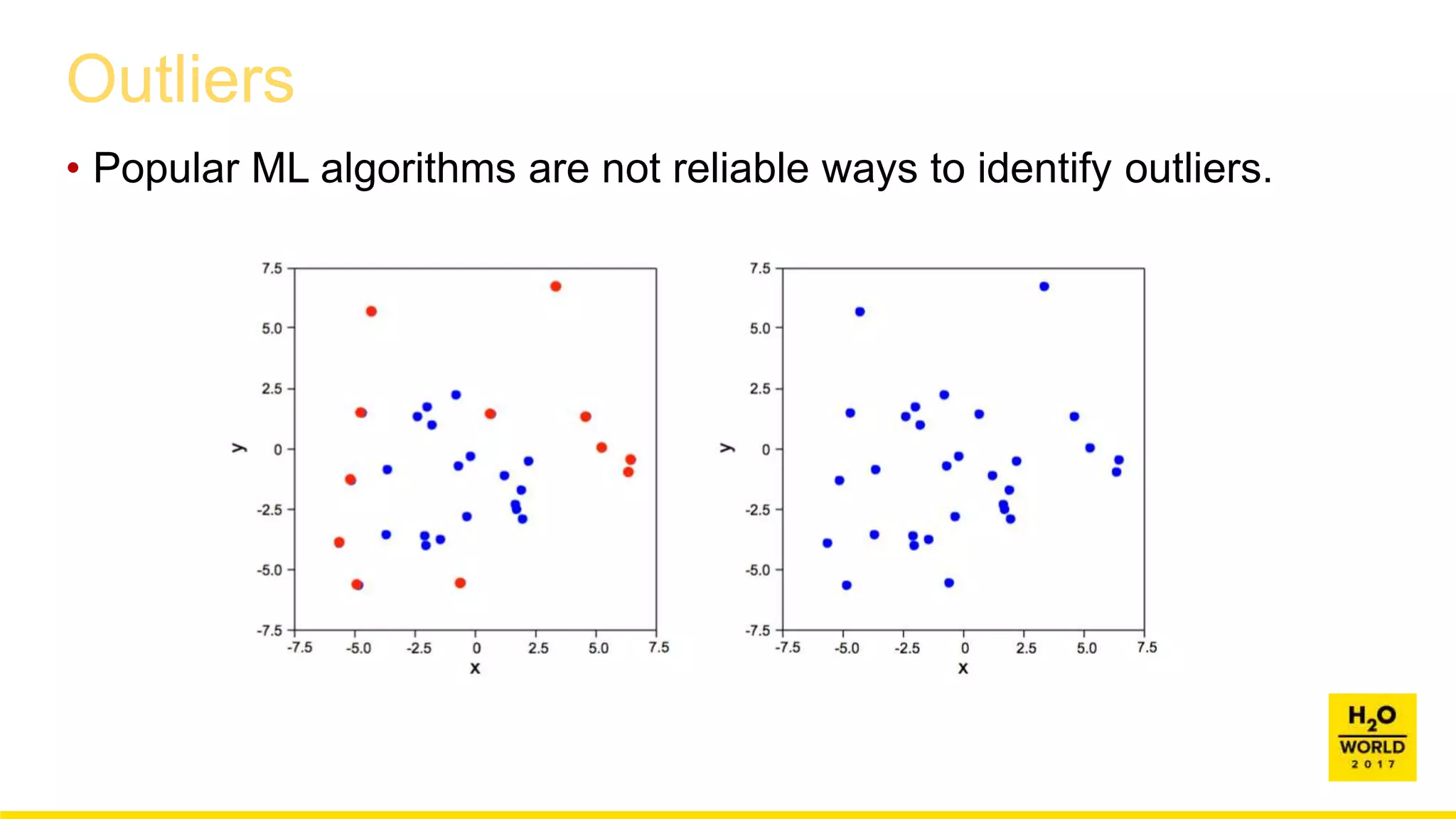
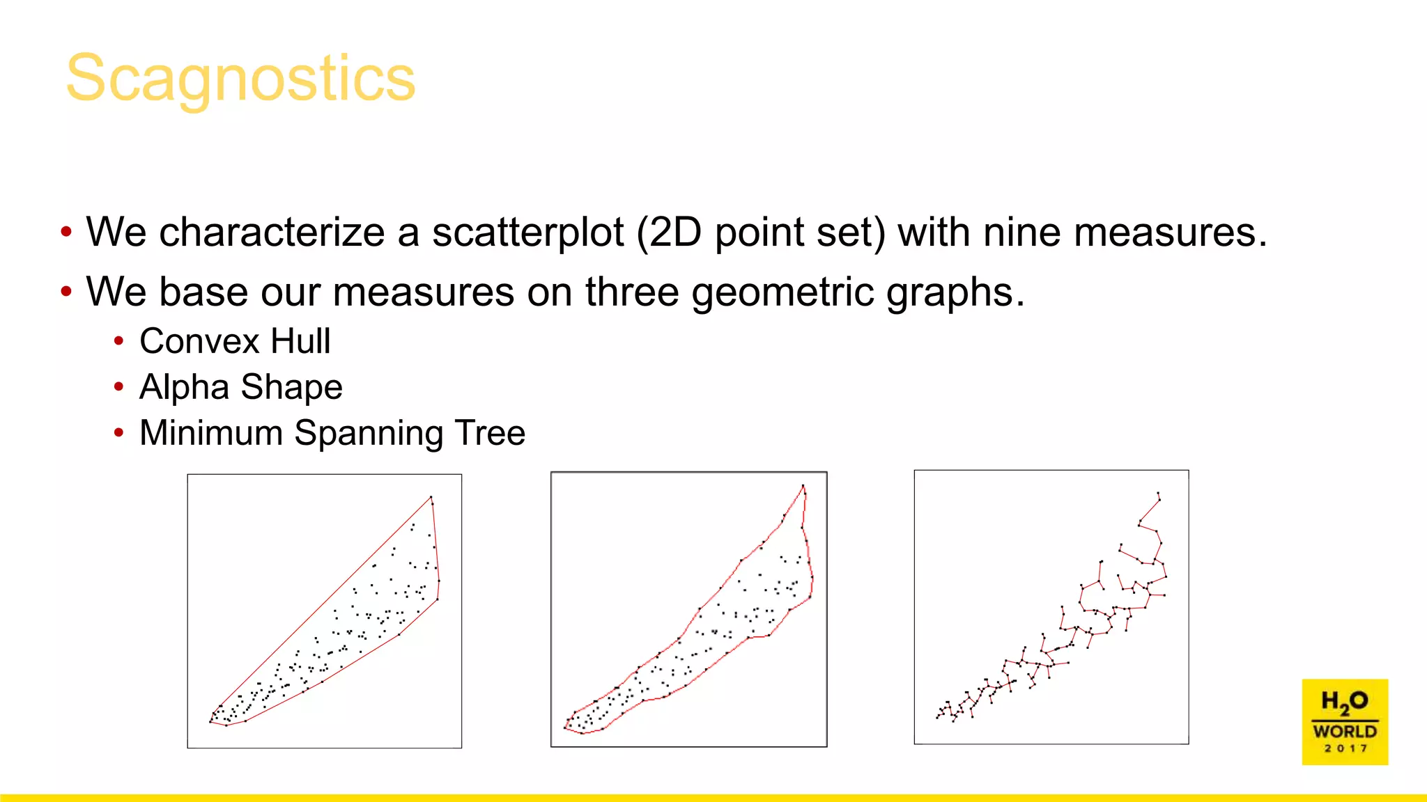
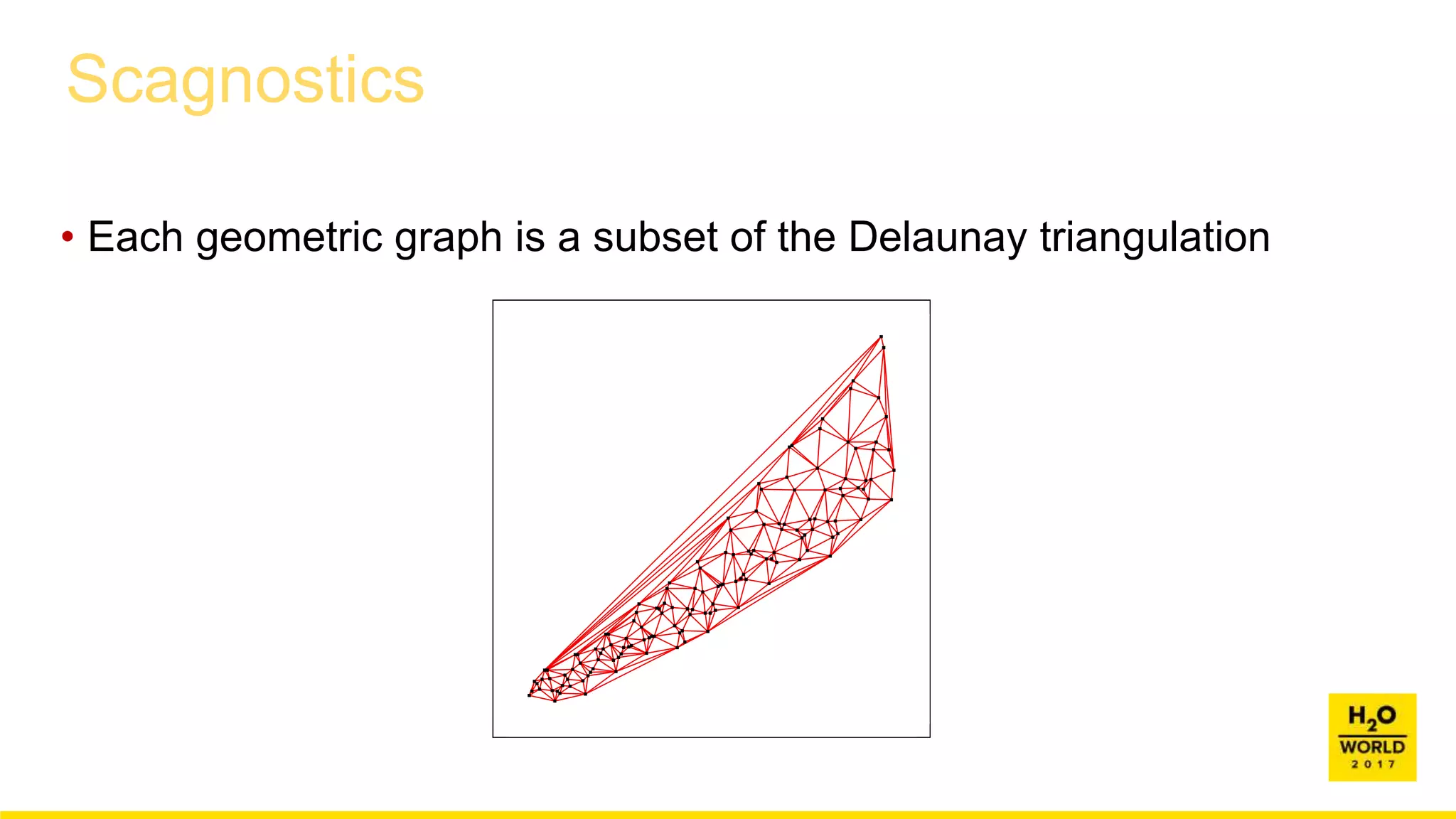


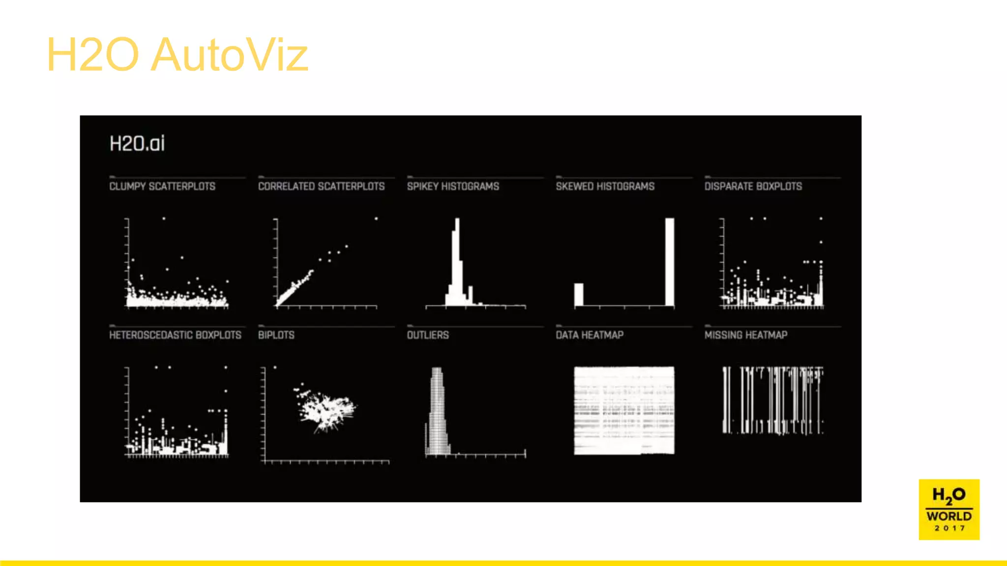


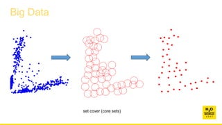
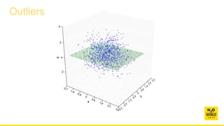
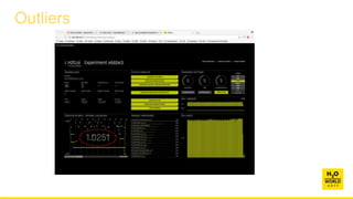
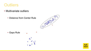
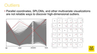
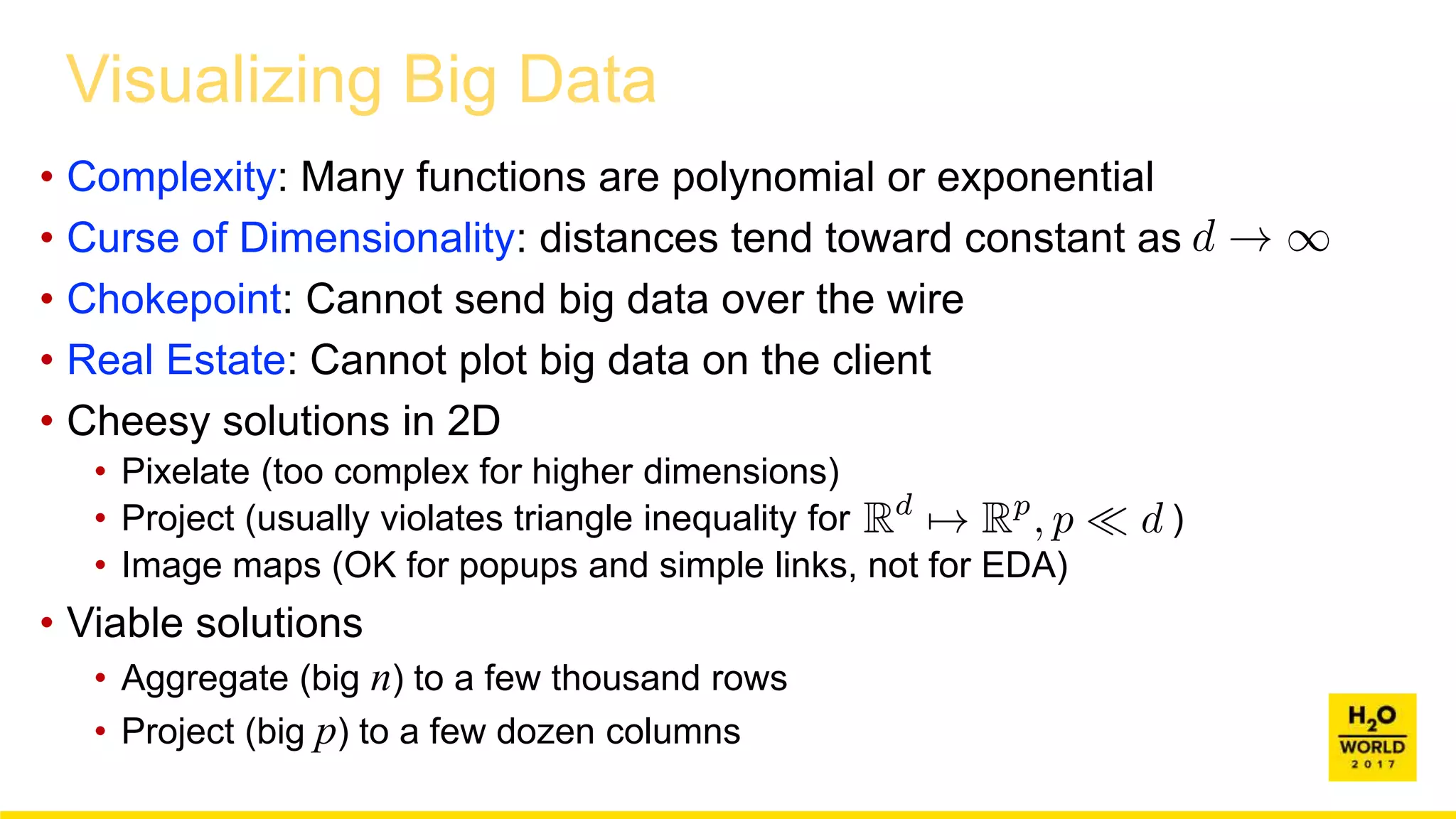
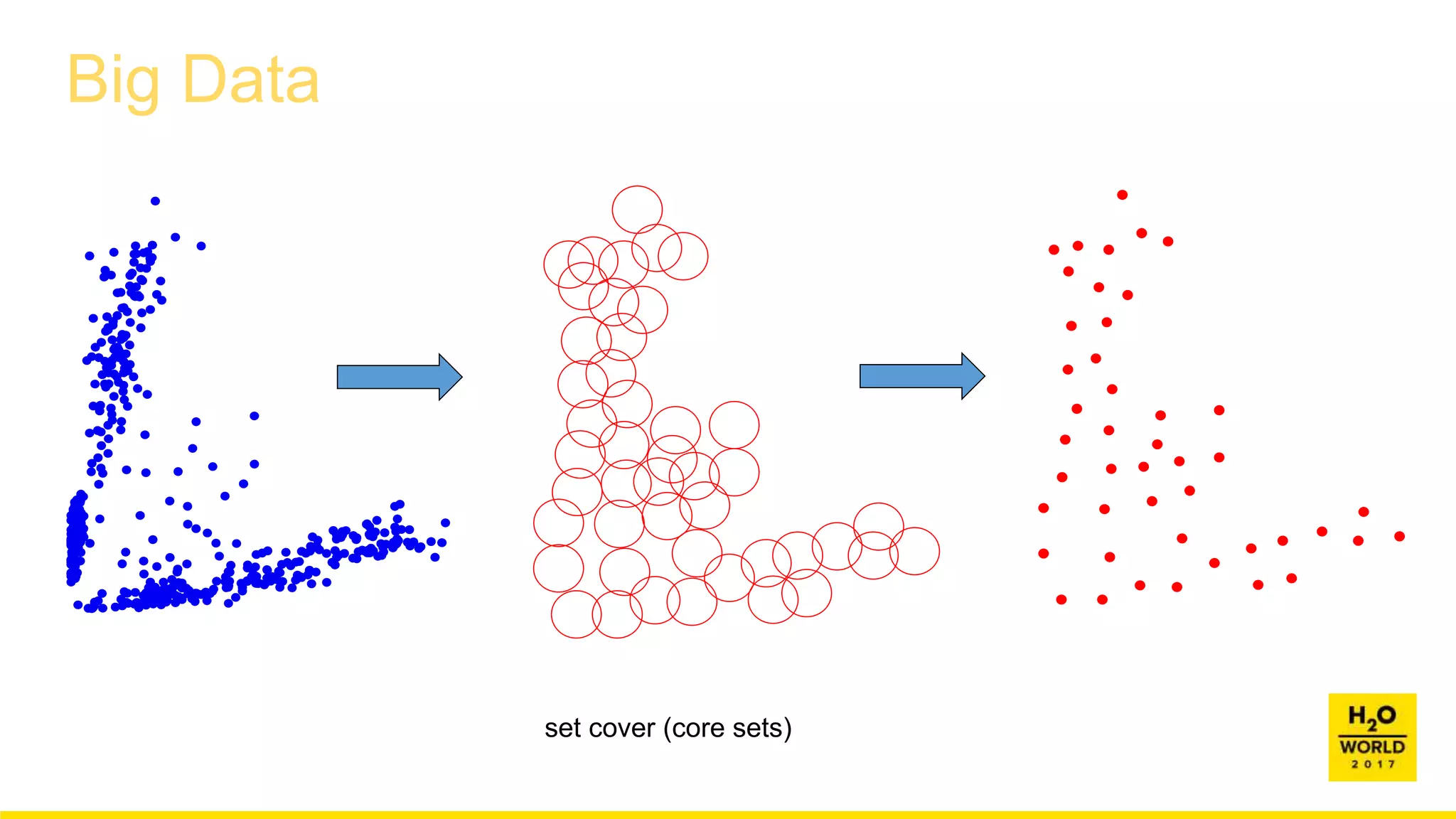
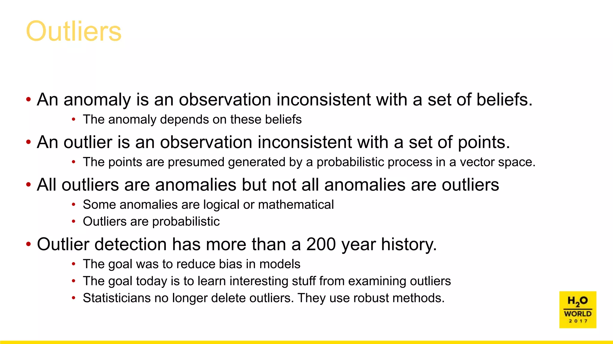
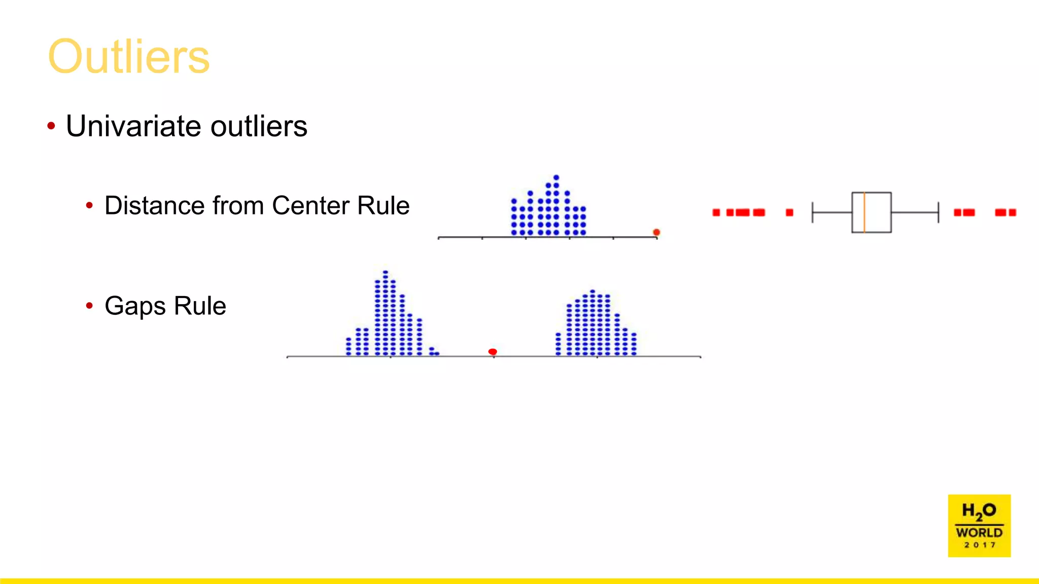
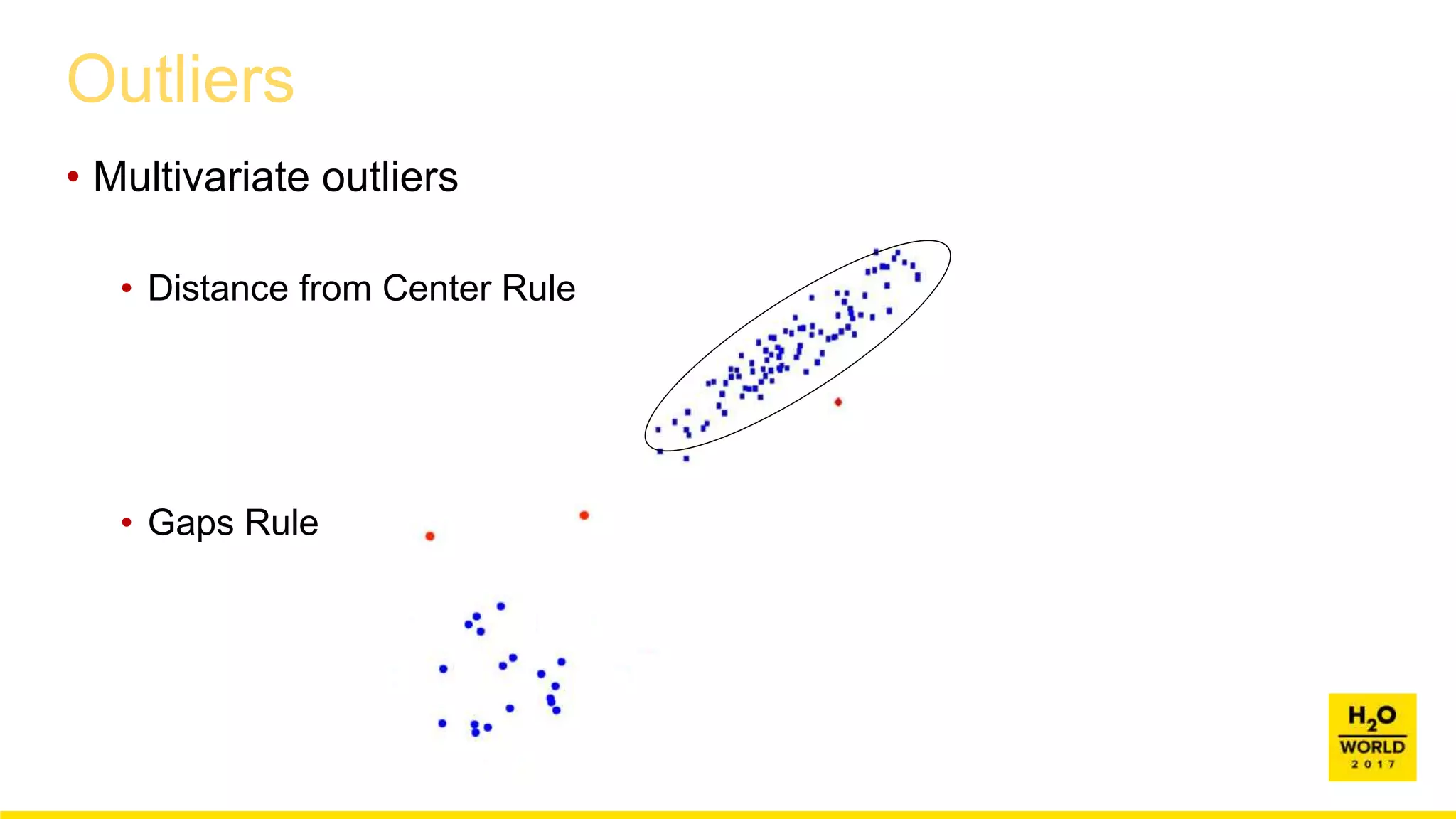
This document discusses automatic visualization of big data and outlier detection in high-dimensional data. It introduces several techniques for visualizing and analyzing big data, including aggregating data to reduce the number of rows/columns, projecting high-dimensional data to lower dimensions, and using core sets to represent large datasets. The document also discusses different types of outliers and algorithms for outlier detection in multivariate data. It notes challenges with visualizing outliers in high dimensions and outlines a process for outlier detection that includes normalization, dimensionality reduction if needed, and fitting an exponential distribution to distances between points.


