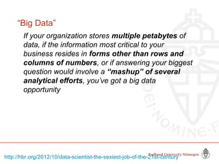
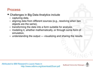
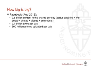
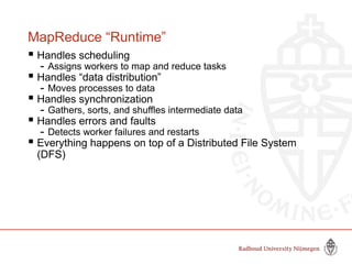
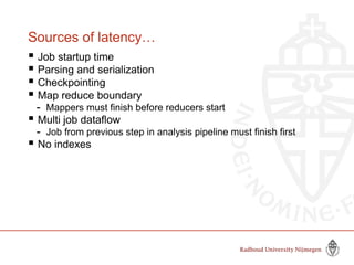
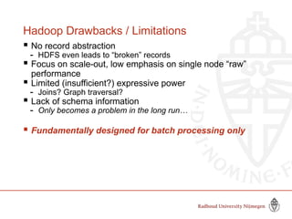
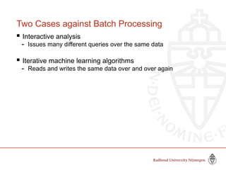
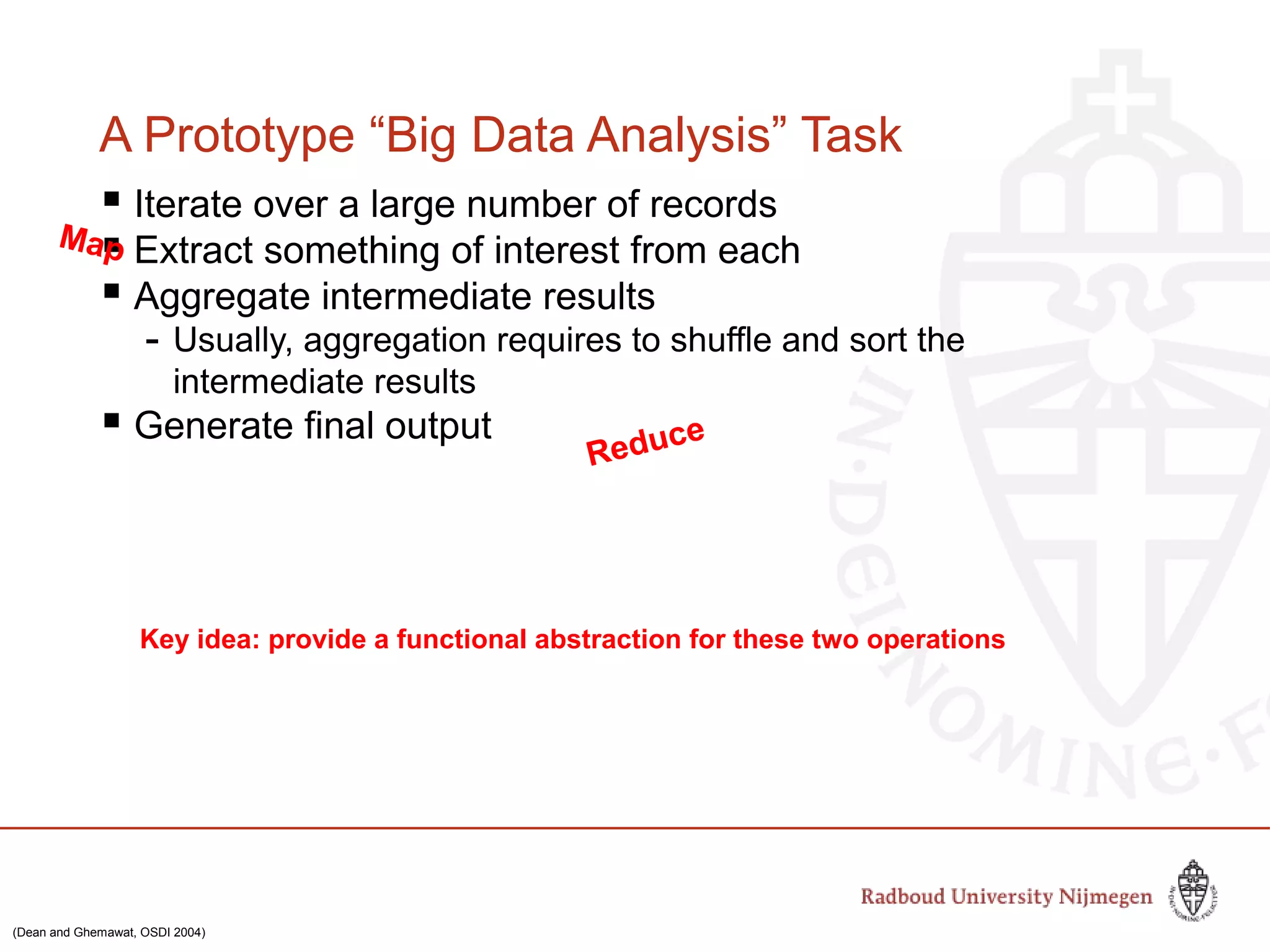
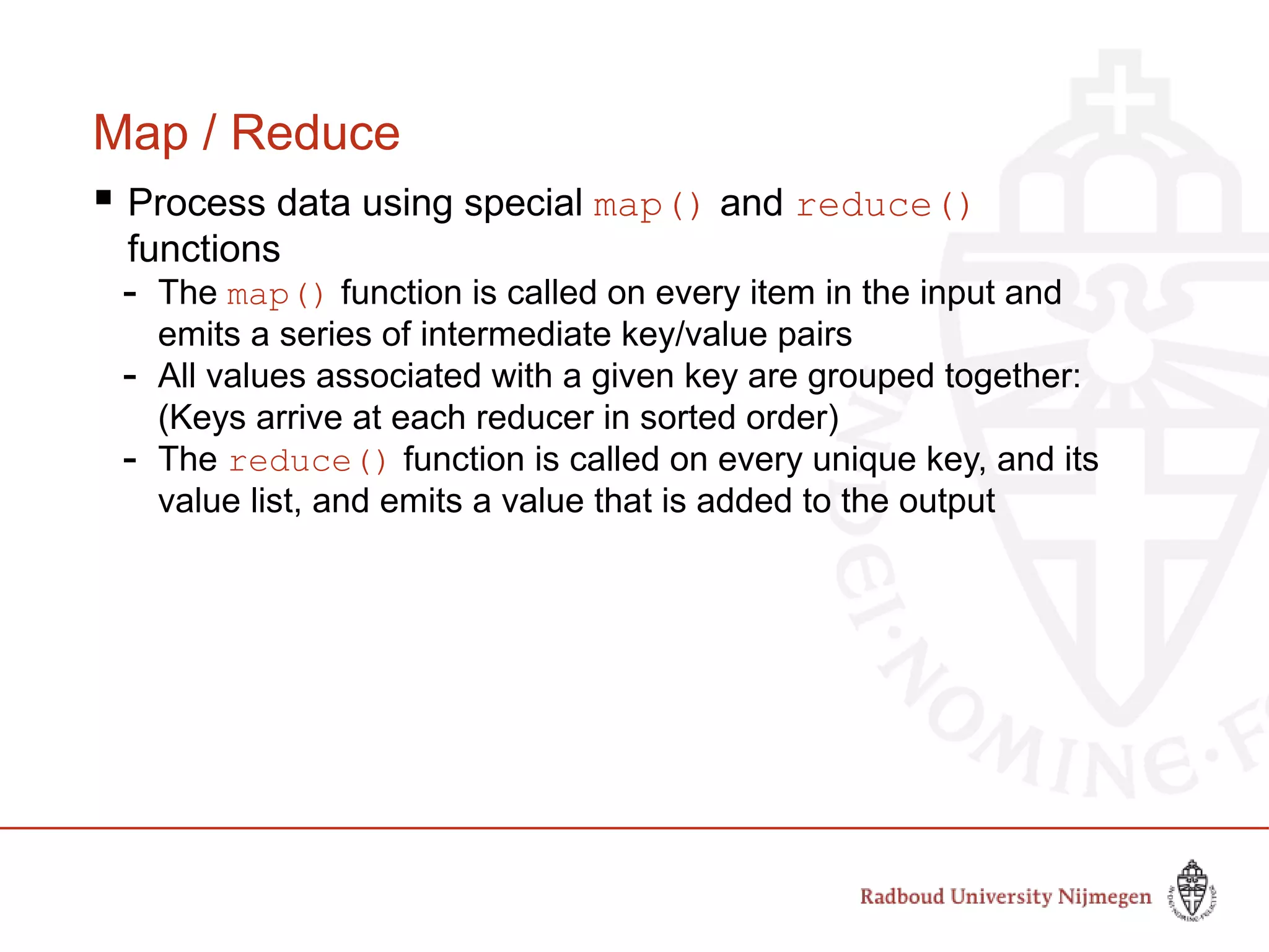
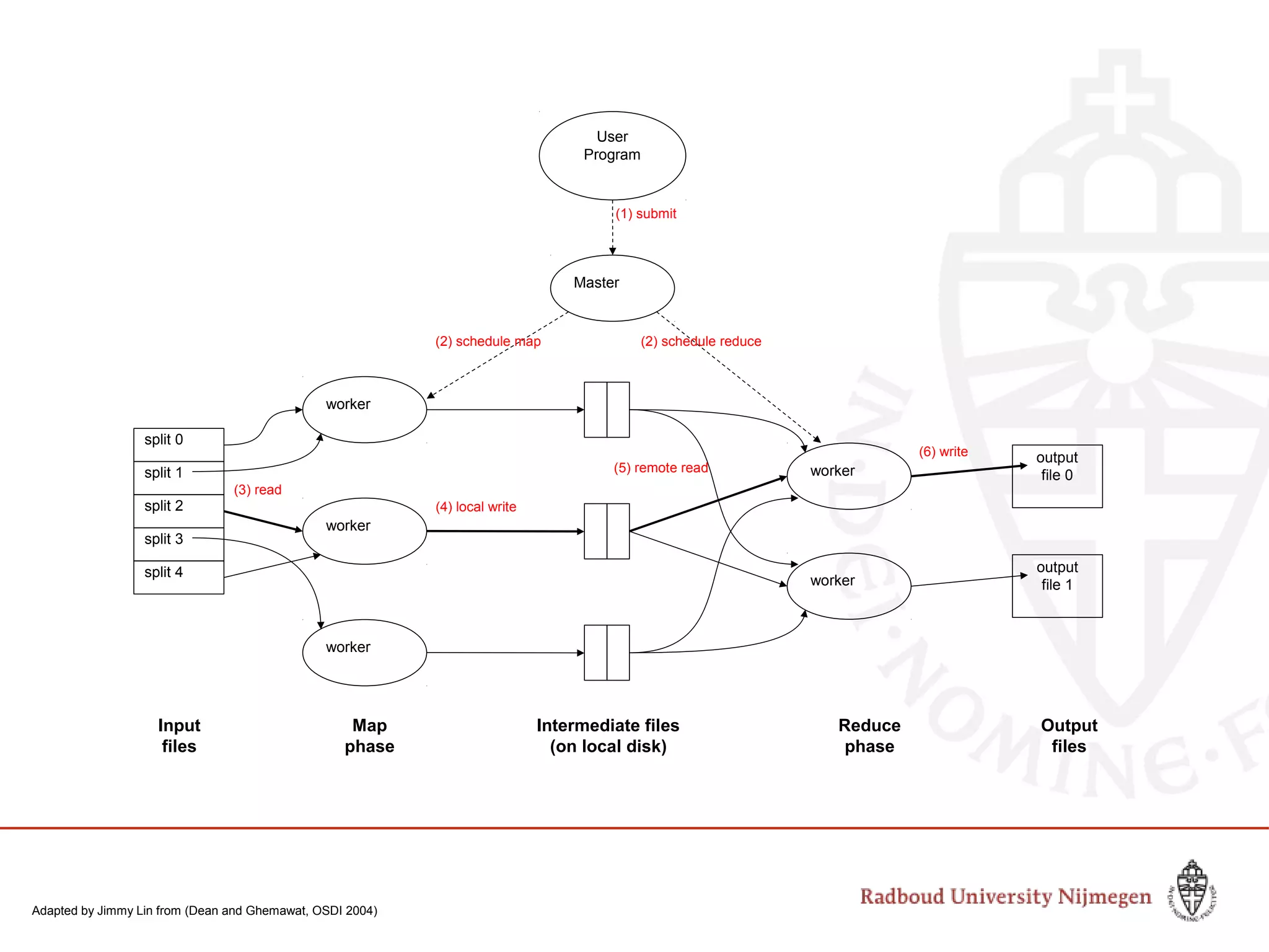
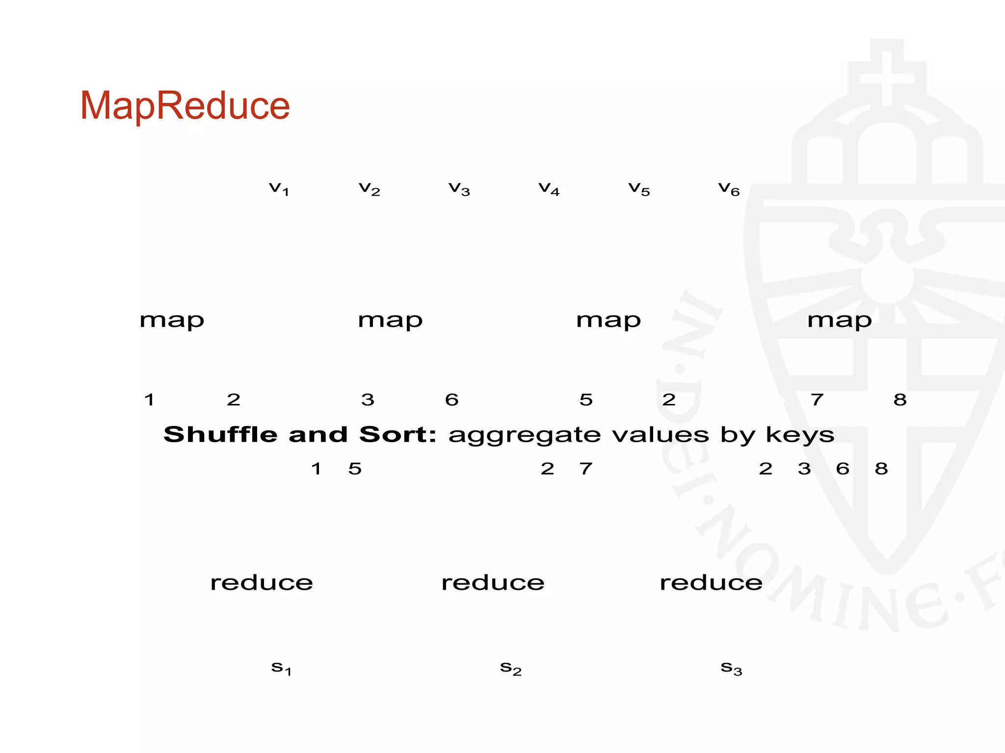
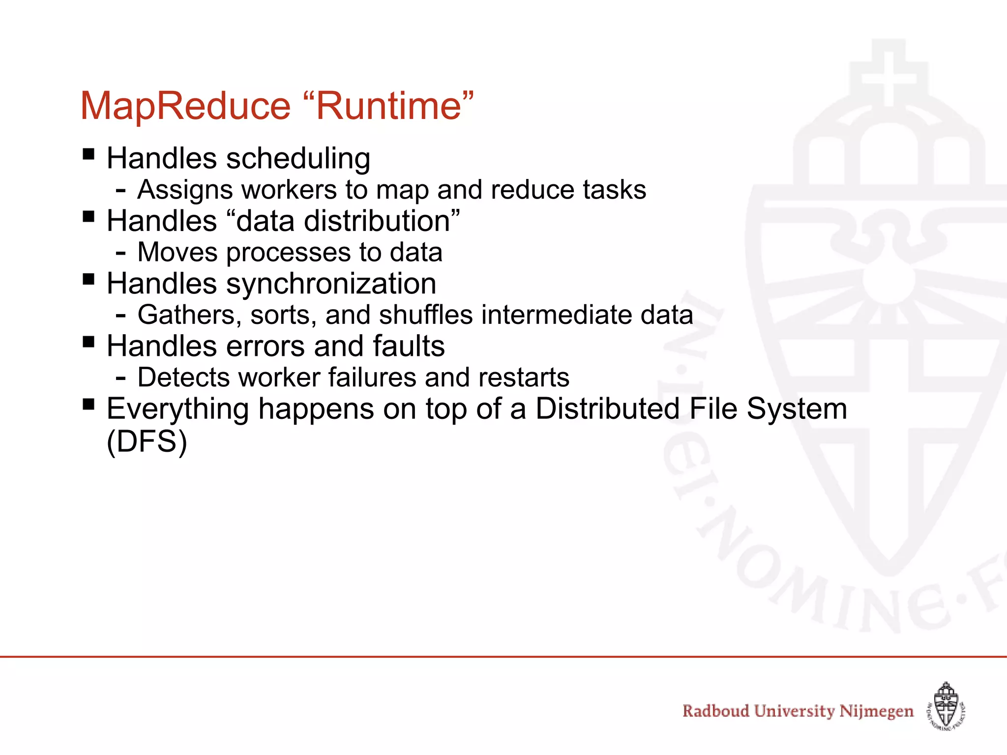
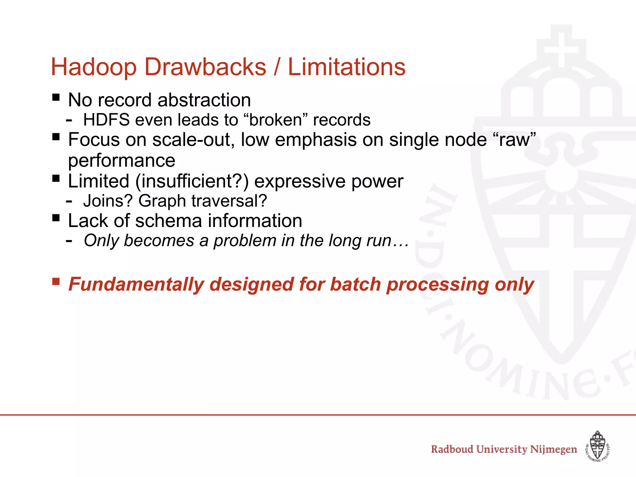
KEMBAR78
Bigdata processing with Spark | PPT
SIKS Big Data Course
Prof.dr.ir. Arjen P. de Vries
arjen@acm.org
Enschede, December 5, 2016
“Big Data”
If your organization stores multiple petabytes of
data, if the information most critical to your
business resides in forms other than rows and
columns of numbers, or if answering your biggest
question would involve a “mashup” of several
analytical efforts, you’ve got a big data
opportunity
http://hbr.org/2012/10/data-scientist-the-sexiest-job-of-the-21st-century
Process
 Challenges in Big Data Analytics include
- capturing data,
- aligning data from different sources (e.g., resolving when two
objects are the same),
- transforming the data into a form suitable for analysis,
- modeling it, whether mathematically, or through some form of
simulation,
- understanding the output — visualizing and sharing the results
Attributed to IBM Research’s Laura Haas in
http://www.odbms.org/download/Zicari.pdf
How big is big?
 Facebook (Aug 2012):
- 2.5 billion content items shared per day (status updates + wall
posts + photos + videos + comments)
- 2.7 billion Likes per day
- 300 million photos uploaded per day
Big is very big!
 100+ petabytes of disk space in one of
FB’s largest Hadoop (HDFS) clusters
 105 terabytes of data scanned via Hive, Facebook’s
Hadoop query language, every 30 minutes
 70,000 queries executed on these databases per day
 500+ terabytes of new data ingested into the databases
every day
http://gigaom.com/data/facebook-is-collecting-your-data-500-terabytes-a-day/
Back of the Envelope
 Note:
“105 terabytes of data scanned every 30 minutes”
 A very very fast disk can do 300 MB/s – so, on one disk,
this would take
(105 TB = 110100480 MB) / 300 (MB/s) =
367Ks =~ 6000m
 So at least 200 disks are used in parallel!
 PS: the June 2010 estimate was that facebook ran on 60K servers
Source: Google
Data Center (is the Computer)
Source: NY Times (6/14/2006), http://www.nytimes.com/2006/06/14/technology/14search.html
FB’s Data Centers
 Suggested further reading:
- http://www.datacenterknowledge.com/the-facebook-data-center-faq/
- http://opencompute.org/
- “Open hardware”: server, storage, and data center
- Claim 38% more efficient and 24% less expensive to build and
run than other state-of-the-art data centers
Building Blocks
Source: Barroso, Clidaras and Hölzle (2013): DOI 10.2200/S00516ED2V01Y201306CAC024
Storage Hierarchy
Source: Barroso, Clidaras and Hölzle (2013): DOI 10.2200/S00516ED2V01Y201306CAC024
Numbers Everyone Should Know
L1 cache reference 0.5 ns
Branch mispredict 5 ns
L2 cache reference 7 ns
Mutex lock/unlock 100 ns
Main memory reference 100 ns
Compress 1K bytes with Zippy 10,000 ns
Send 2K bytes over 1 Gbps network 20,000 ns
Read 1 MB sequentially from memory 250,000 ns
Round trip within same datacenter 500,000 ns
Disk seek 10,000,000 ns
Read 1 MB sequentially from network 10,000,000 ns
Read 1 MB sequentially from disk 30,000,000 ns
Send packet CA->Netherlands->CA 150,000,000 ns
According to Jeff Dean
Storage Hierarchy
Source: Barroso, Clidaras and Hölzle (2013): DOI 10.2200/S00516ED2V01Y201306CAC024
Storage Hierarchy
Source: Barroso, Clidaras and Hölzle (2013): DOI 10.2200/S00516ED2V01Y201306CAC024
Quiz Time!!
 Consider a 1 TB database with 100 byte records
- We want to update 1 percent of the records
Plan A:
Seek to the records and make the updates
Plan B:
Write out a new database that includes the updates
Source: Ted Dunning, on Hadoop mailing list
Seeks vs. Scans
 Consider a 1 TB database with 100 byte records
- We want to update 1 percent of the records
 Scenario 1: random access
- Each update takes ~30 ms (seek, read, write)
- 108
updates = ~35 days
 Scenario 2: rewrite all records
- Assume 100 MB/s throughput
- Time = 5.6 hours(!)
 Lesson: avoid random seeks!
In words of Prof. Peter Boncz (CWI & VU):
“Latency is the enemy”
Source: Ted Dunning, on Hadoop mailing list
Programming for Big Data the Data Center
Emerging Big Data Systems
 Distributed
 Shared-nothing
- None of the resources are logically shared between processes
 Data parallel
- Exactly the same task is performed on different pieces of the
data
Shared-nothing
 A collection of independent, possibly virtual, machines,
each with local disk and local main memory, connected
together on a high-speed network
- Possible trade-off: large number of low-end servers instead of
small number of high-end ones
@UT~1990
Data Parallel
 Remember:
0.5ns (L1) vs.
500,000ns (round trip in datacenter)
Δ is 6 orders in magnitude!
 With huge amounts of data (and resources necessary to
process it), we simply cannot expect to ship the data to
the application – the application logic needs to ship to the
data!
Gray’s Laws
How to approach data engineering challenges for large-scale
scientific datasets:
1. Scientific computing is becoming increasingly data intensive
2. The solution is in a “scale-out” architecture
3. Bring computations to the data, rather than data to the
computations
4. Start the design with the “20 queries”
5. Go from “working to working”
See:
http://research.microsoft.com/en-us/collaboration/fourthparadigm/4th_paradigm_book_part1_szalay.pdf
Distributed File System (DFS)
 Exact location of data is unknown to the programmer
 Programmer writes a program on an abstraction level
above that of low level data
- however, notice that abstraction level offered is usually still
rather low…
GFS: Assumptions
 Commodity hardware over “exotic” hardware
- Scale “out”, not “up”
 High component failure rates
- Inexpensive commodity components fail all the time
 “Modest” number of huge files
- Multi-gigabyte files are common, if not encouraged
 Files are write-once, mostly appended to
- Perhaps concurrently
 Large streaming reads over random access
- High sustained throughput over low latency
GFS slides adapted from material by (Ghemawat et al., SOSP 2003)
GFS: Design Decisions
 Files stored as chunks
- Fixed size (64MB)
 Reliability through replication
- Each chunk replicated across 3+ chunkservers
 Single master to coordinate access, keep metadata
- Simple centralized management
 No data caching
- Little benefit due to large datasets, streaming reads
 Simplify the API
- Push some of the issues onto the client (e.g., data layout)
HDFS = GFS clone (same basic ideas)
A Prototype “Big Data Analysis” Task
 Iterate over a large number of records
 Extract something of interest from each
 Aggregate intermediate results
- Usually, aggregation requires to shuffle and sort the
intermediate results
 Generate final output
Key idea: provide a functional abstraction for these two operations
Map
Reduce
(Dean and Ghemawat, OSDI 2004)
Map / Reduce
“A simple and powerful interface that enables automatic
parallelization and distribution of large-scale computations,
combined with an implementation of this interface that
achieves high performance on large clusters of commodity
PCs”
MapReduce: Simplified Data Processing on Large
Clusters, Jeffrey Dean and Sanjay Ghemawat, 2004
http://research.google.com/archive/mapreduce.html
MR Implementations
 Google “invented” their MR system, a proprietary
implementation in C++
- Bindings in Java, Python
 Hadoop is an open-source re-implementation in Java
- Original development led by Yahoo
- Now an Apache open source project
- Emerging as the de facto big data stack
- Rapidly expanding software ecosystem
Map / Reduce
 Process data using special map() and reduce()
functions
- The map() function is called on every item in the input and
emits a series of intermediate key/value pairs
- All values associated with a given key are grouped together:
(Keys arrive at each reducer in sorted order)
- The reduce() function is called on every unique key, and its
value list, and emits a value that is added to the output
split 0
split 1
split 2
split 3
split 4
worker
worker
worker
worker
worker
Master
User
Program
output
file 0
output
file 1
(1) submit
(2) schedule map (2) schedule reduce
(3) read
(4) local write
(5) remote read
(6) write
Input
files
Map
phase
Intermediate files
(on local disk)
Reduce
phase
Output
files
Adapted by Jimmy Lin from (Dean and Ghemawat, OSDI 2004)
MapReduce
mapmap map map
Shuffle and Sort: aggregate values by keys
reduce reduce reduce
k1 k2 k3 k4 k5 k6v1 v2 v3 v4 v5 v6
ba 1 2 c c3 6 a c5 2 b c7 8
a 1 5 b 2 7 c 2 3 6 8
r1 s1 r2 s2 r3 s3
mapmap map map
Shuffle and Sort: aggregate values by keys
reduce reduce reduce
k1 k2 k3 k4 k5 k6v1 v2 v3 v4 v5 v6k1 k2 k3 k4 k5 k6v1 v2 v3 v4 v5 v6
ba 1 2ba 1 2 c c3 6c c3 6 a c5 2a c5 2 b c7 8b c7 8
a 1 5a 1 5 b 2 7b 2 7 c 2 3 6 8c 2 3 6 8
r1 s1r1 s1 r2 s2r2 s2 r3 s3r3 s3
MapReduce “Runtime”
 Handles scheduling
- Assigns workers to map and reduce tasks
 Handles “data distribution”
- Moves processes to data
 Handles synchronization
- Gathers, sorts, and shuffles intermediate data
 Handles errors and faults
- Detects worker failures and restarts
 Everything happens on top of a Distributed File System
(DFS)
Q: “Hadoop the Answer?”
Data Juggling
 Operational reality of many organizations is that Big Data
is constantly being pumped between different systems:
- Key-value stores
- General-purpose distributed file system
- (Distributed) DBMSs
- Custom (distributed) file organizations
Q: “Hadoop the Answer?”
 Not that easy to write efficient and scalable code!
Controlling Execution
 Cleverly-constructed data structures for keys and values
- Carry partial results together through the pipeline
 Sort order of intermediate keys
- Control order in which reducers process keys
 Partitioning of the key space
- Control which reducer processes which keys
 Preserving state in mappers and reducers
- Capture dependencies across multiple keys and values
Hadoop’s Deficiencies
Sources of latency…
 Job startup time
 Parsing and serialization
 Checkpointing
 Map reduce boundary
- Mappers must finish before reducers start
 Multi job dataflow
- Job from previous step in analysis pipeline must finish first
 No indexes
Hadoop Drawbacks / Limitations
 No record abstraction
- HDFS even leads to “broken” records
 Focus on scale-out, low emphasis on single node “raw”
performance
 Limited (insufficient?) expressive power
- Joins? Graph traversal?
 Lack of schema information
- Only becomes a problem in the long run…
 Fundamentally designed for batch processing only
Two Cases against Batch Processing
 Interactive analysis
- Issues many different queries over the same data
 Iterative machine learning algorithms
- Reads and writes the same data over and over again
Slow due to replication, serialization, and disk IO
Input
query 1query 1
query 2query 2
query 3query 3
result 1
result 2
result 3
. . .
HDFS
read
iter. 2iter. 2 . . .
HDFS
read
HDFS
write
Data Sharing (Hadoop)
iter. 1iter. 1
HDFS
read
HDFS
write
Input
iter. 1iter. 1
HDFS
read
HDFS
write
Input
Intermezzo…
iter. 2iter. 2 . . .
Distributed
memory
Input
query 1query 1
query 2query 2
query 3query 3
. . .
one-time
processing
10-100× faster than network and disk
Data Sharing (Spark)
iter. 1iter. 1
Input
iter. 1iter. 1
Input
Challenge
 Distributed memory abstraction must be
- Fault-tolerant
- Efficient in large commodity clusters
How do we design a programming interface
that can provide fault tolerance efficiently?
Challenge
 Previous distributed storage abstractions have offered an
interface based on fine-grained updates
- Reads and writes to cells in a table
- E.g. key-value stores, databases, distributed memory
 Requires replicating data or update logs across nodes for
fault tolerance
- Expensive for data-intensive apps (i.e., Big Data)
Spark Programming Model
Key idea: Resilient Distributed Datasets (RDDs)
- Distributed collections of objects
- Cached in memory across cluster nodes, upon request
- Parallel operators to manipulate data in RDDs
- Automatic reconstruction of intermediate results upon failure
Interface
- Clean language-integrated API in Scala
- Can be used interactively from Scala console
RDDs: Batch Processing
 Set-oriented operations (instead of tuple-oriented)
- Same basic principle as relational databases, key for efficient
query processing
 A nested relational model
- Allows for complex values that may need to be “flattened” for
further processing
- E.g.:
map vs. flatMap
RDD Operations
Great documentation!
http://spark.apache.org/docs/latest/programming-
guide.html#rdd-operations
Example: Log Mining
 Load error messages from a log into memory, then interactively
search for various patterns
lines = spark.textFile(“hdfs://...”)
errors = lines.filter(_.startsWith(“ERROR”))
messages = errors.map(_.split(‘t’)(2))
cachedMsgs = messages.cache()
Block 1Block 1
Block 2Block 2
Block 3Block 3
WorkerWorker
WorkerWorker
WorkerWorker
DriverDriver
cachedMsgs.filter(_.contains(“foo”)).count
cachedMsgs.filter(_.contains(“bar”)).count
. . .
tasks
results
Cache 1Cache 1
Cache 2Cache 2
Cache 3Cache 3
Base RDDBase RDD
Transformed RDDTransformed RDD
ActionAction
Result: full-text search of Wikipedia
in <1 sec (vs 20 sec for on-disk data)
Result: scaled to 1 TB data in 5-7 sec
(vs 170 sec for on-disk data)
Slide by Matei Zaharia, creator Spark, http://spark-project.org
Example: Logistic Regression val data =
spark.textFile(...).map(readPoint).cache()
 var w = Vector.random(D)
 for (i <- 1 to ITERATIONS) {
 val gradient = data.map(p =>
 (1 / (1 + exp(-p.y*(w dot p.x))) - 1) * p.y *
p.x
 ).reduce(_ + _)
 w -= gradient
 }
 println("Final w: " + w)
Initial parameter vectorInitial parameter vector
Repeated MapReduce steps
to do gradient descent
Repeated MapReduce steps
to do gradient descent
Load data in memory onceLoad data in memory once
Slide by Matei Zaharia, creator Spark, http://spark-project.org
Logistic Regression Performance
127 s / iteration
first iteration 174 s
further iterations 6 s
Slide by Matei Zaharia, creator Spark, http://spark-project.org
Example Job
val sc = new SparkContext(
“spark://...”, “MyJob”, home, jars)
val file = sc.textFile(“hdfs://...”)
val errors = file.filter(_.contains(“ERROR”))
errors.cache()
errors.count()
Resilient distributed
datasets (RDDs)
Resilient distributed
datasets (RDDs)
ActionAction
Transformations build up a DAG, but don’t “do
anything”
54
RDD Graph
HadoopRDD
path = hdfs://...
HadoopRDD
path = hdfs://...
FilteredRDD
func = _.contains(…)
shouldCache = true
FilteredRDD
func = _.contains(…)
shouldCache = true
file:
errors:
Partition-level view:Dataset-level view:
Task 1Task 2 ...
Data Locality
First run: data not in cache, so use HadoopRDD’s
locality prefs (from HDFS)
Second run: FilteredRDD is in cache, so use its
locations
If something falls out of cache, go back to HDFS
Resilient Distributed Datasets (RDDs)
 Offer an interface based on coarse-grained transformations
(e.g. map, group-by, join)
 Allows for efficient fault recovery using lineage
- Log one operation to apply to many elements
- Recompute lost partitions of dataset on failure
- No cost if nothing fails
RDD Fault Tolerance
 RDDs maintain lineage information that can be used to
reconstruct lost partitions
 Ex:
messages = textFile(...).filter(_.startsWith(“ERROR”))
.map(_.split(‘t’)(2))
HDFSFileHDFSFile FilteredRDDFilteredRDD MappedRDDMappedRDD
filter
(func = _.startsWith(...))
map
(func = _.split(...))
Slide by Matei Zaharia, creator Spark, http://spark-project.org
RDD Representation
 Simple common interface:
- Set of partitions
- Preferred locations for each partition
- List of parent RDDs
- Function to compute a partition given parents
- Optional partitioning info
 Allows capturing wide range of transformations
 Users can easily add new transformations
Slide by Matei Zaharia, creator Spark, http://spark-project.org
RDDs in More Detail
RDDs additionally provide:
- Control over partitioning, which can be used to optimize data
placement across queries.
- usually more efficient than the sort-based approach of Map
Reduce
- Control over persistence (e.g. store on disk vs in RAM)
- Fine-grained reads (treat RDD as a big table)
Slide by Matei Zaharia, creator Spark, http://spark-project.org
Wrap-up: Spark
 Avoid materialization of intermediate results
 Recomputation is a viable alternative for replication to
provide fault tolerance
 A good and user-friendly (i.e., programmer-friendly) API
helps gain traction very fast
- In few years, Spark has become the default tool for deploying
code on clusters
Thanks
 Matei Zaharia, MIT (https://people.csail.mit.edu/matei/)
 http://spark-project.org

Bigdata processing with Spark

  • 1.
    SIKS Big DataCourse Prof.dr.ir. Arjen P. de Vries arjen@acm.org Enschede, December 5, 2016
  • 2.
    “Big Data” If yourorganization stores multiple petabytes of data, if the information most critical to your business resides in forms other than rows and columns of numbers, or if answering your biggest question would involve a “mashup” of several analytical efforts, you’ve got a big data opportunity http://hbr.org/2012/10/data-scientist-the-sexiest-job-of-the-21st-century
  • 3.
    Process  Challenges inBig Data Analytics include - capturing data, - aligning data from different sources (e.g., resolving when two objects are the same), - transforming the data into a form suitable for analysis, - modeling it, whether mathematically, or through some form of simulation, - understanding the output — visualizing and sharing the results Attributed to IBM Research’s Laura Haas in http://www.odbms.org/download/Zicari.pdf
  • 4.
    How big isbig?  Facebook (Aug 2012): - 2.5 billion content items shared per day (status updates + wall posts + photos + videos + comments) - 2.7 billion Likes per day - 300 million photos uploaded per day
  • 5.
    Big is verybig!  100+ petabytes of disk space in one of FB’s largest Hadoop (HDFS) clusters  105 terabytes of data scanned via Hive, Facebook’s Hadoop query language, every 30 minutes  70,000 queries executed on these databases per day  500+ terabytes of new data ingested into the databases every day http://gigaom.com/data/facebook-is-collecting-your-data-500-terabytes-a-day/
  • 6.
    Back of theEnvelope  Note: “105 terabytes of data scanned every 30 minutes”  A very very fast disk can do 300 MB/s – so, on one disk, this would take (105 TB = 110100480 MB) / 300 (MB/s) = 367Ks =~ 6000m  So at least 200 disks are used in parallel!  PS: the June 2010 estimate was that facebook ran on 60K servers
  • 7.
    Source: Google Data Center(is the Computer)
  • 8.
    Source: NY Times(6/14/2006), http://www.nytimes.com/2006/06/14/technology/14search.html
  • 9.
    FB’s Data Centers Suggested further reading: - http://www.datacenterknowledge.com/the-facebook-data-center-faq/ - http://opencompute.org/ - “Open hardware”: server, storage, and data center - Claim 38% more efficient and 24% less expensive to build and run than other state-of-the-art data centers
  • 10.
    Building Blocks Source: Barroso,Clidaras and Hölzle (2013): DOI 10.2200/S00516ED2V01Y201306CAC024
  • 11.
    Storage Hierarchy Source: Barroso,Clidaras and Hölzle (2013): DOI 10.2200/S00516ED2V01Y201306CAC024
  • 12.
    Numbers Everyone ShouldKnow L1 cache reference 0.5 ns Branch mispredict 5 ns L2 cache reference 7 ns Mutex lock/unlock 100 ns Main memory reference 100 ns Compress 1K bytes with Zippy 10,000 ns Send 2K bytes over 1 Gbps network 20,000 ns Read 1 MB sequentially from memory 250,000 ns Round trip within same datacenter 500,000 ns Disk seek 10,000,000 ns Read 1 MB sequentially from network 10,000,000 ns Read 1 MB sequentially from disk 30,000,000 ns Send packet CA->Netherlands->CA 150,000,000 ns According to Jeff Dean
  • 13.
    Storage Hierarchy Source: Barroso,Clidaras and Hölzle (2013): DOI 10.2200/S00516ED2V01Y201306CAC024
  • 14.
    Storage Hierarchy Source: Barroso,Clidaras and Hölzle (2013): DOI 10.2200/S00516ED2V01Y201306CAC024
  • 15.
    Quiz Time!!  Considera 1 TB database with 100 byte records - We want to update 1 percent of the records Plan A: Seek to the records and make the updates Plan B: Write out a new database that includes the updates Source: Ted Dunning, on Hadoop mailing list
  • 16.
    Seeks vs. Scans Consider a 1 TB database with 100 byte records - We want to update 1 percent of the records  Scenario 1: random access - Each update takes ~30 ms (seek, read, write) - 108 updates = ~35 days  Scenario 2: rewrite all records - Assume 100 MB/s throughput - Time = 5.6 hours(!)  Lesson: avoid random seeks! In words of Prof. Peter Boncz (CWI & VU): “Latency is the enemy” Source: Ted Dunning, on Hadoop mailing list
  • 17.
    Programming for BigData the Data Center
  • 18.
    Emerging Big DataSystems  Distributed  Shared-nothing - None of the resources are logically shared between processes  Data parallel - Exactly the same task is performed on different pieces of the data
  • 19.
    Shared-nothing  A collectionof independent, possibly virtual, machines, each with local disk and local main memory, connected together on a high-speed network - Possible trade-off: large number of low-end servers instead of small number of high-end ones
  • 21.
  • 22.
    Data Parallel  Remember: 0.5ns(L1) vs. 500,000ns (round trip in datacenter) Δ is 6 orders in magnitude!  With huge amounts of data (and resources necessary to process it), we simply cannot expect to ship the data to the application – the application logic needs to ship to the data!
  • 23.
    Gray’s Laws How toapproach data engineering challenges for large-scale scientific datasets: 1. Scientific computing is becoming increasingly data intensive 2. The solution is in a “scale-out” architecture 3. Bring computations to the data, rather than data to the computations 4. Start the design with the “20 queries” 5. Go from “working to working” See: http://research.microsoft.com/en-us/collaboration/fourthparadigm/4th_paradigm_book_part1_szalay.pdf
  • 24.
    Distributed File System(DFS)  Exact location of data is unknown to the programmer  Programmer writes a program on an abstraction level above that of low level data - however, notice that abstraction level offered is usually still rather low…
  • 25.
    GFS: Assumptions  Commodityhardware over “exotic” hardware - Scale “out”, not “up”  High component failure rates - Inexpensive commodity components fail all the time  “Modest” number of huge files - Multi-gigabyte files are common, if not encouraged  Files are write-once, mostly appended to - Perhaps concurrently  Large streaming reads over random access - High sustained throughput over low latency GFS slides adapted from material by (Ghemawat et al., SOSP 2003)
  • 26.
    GFS: Design Decisions Files stored as chunks - Fixed size (64MB)  Reliability through replication - Each chunk replicated across 3+ chunkservers  Single master to coordinate access, keep metadata - Simple centralized management  No data caching - Little benefit due to large datasets, streaming reads  Simplify the API - Push some of the issues onto the client (e.g., data layout) HDFS = GFS clone (same basic ideas)
  • 27.
    A Prototype “BigData Analysis” Task  Iterate over a large number of records  Extract something of interest from each  Aggregate intermediate results - Usually, aggregation requires to shuffle and sort the intermediate results  Generate final output Key idea: provide a functional abstraction for these two operations Map Reduce (Dean and Ghemawat, OSDI 2004)
  • 28.
    Map / Reduce “Asimple and powerful interface that enables automatic parallelization and distribution of large-scale computations, combined with an implementation of this interface that achieves high performance on large clusters of commodity PCs” MapReduce: Simplified Data Processing on Large Clusters, Jeffrey Dean and Sanjay Ghemawat, 2004 http://research.google.com/archive/mapreduce.html
  • 29.
    MR Implementations  Google“invented” their MR system, a proprietary implementation in C++ - Bindings in Java, Python  Hadoop is an open-source re-implementation in Java - Original development led by Yahoo - Now an Apache open source project - Emerging as the de facto big data stack - Rapidly expanding software ecosystem
  • 30.
    Map / Reduce Process data using special map() and reduce() functions - The map() function is called on every item in the input and emits a series of intermediate key/value pairs - All values associated with a given key are grouped together: (Keys arrive at each reducer in sorted order) - The reduce() function is called on every unique key, and its value list, and emits a value that is added to the output
  • 31.
    split 0 split 1 split2 split 3 split 4 worker worker worker worker worker Master User Program output file 0 output file 1 (1) submit (2) schedule map (2) schedule reduce (3) read (4) local write (5) remote read (6) write Input files Map phase Intermediate files (on local disk) Reduce phase Output files Adapted by Jimmy Lin from (Dean and Ghemawat, OSDI 2004)
  • 32.
    MapReduce mapmap map map Shuffleand Sort: aggregate values by keys reduce reduce reduce k1 k2 k3 k4 k5 k6v1 v2 v3 v4 v5 v6 ba 1 2 c c3 6 a c5 2 b c7 8 a 1 5 b 2 7 c 2 3 6 8 r1 s1 r2 s2 r3 s3 mapmap map map Shuffle and Sort: aggregate values by keys reduce reduce reduce k1 k2 k3 k4 k5 k6v1 v2 v3 v4 v5 v6k1 k2 k3 k4 k5 k6v1 v2 v3 v4 v5 v6 ba 1 2ba 1 2 c c3 6c c3 6 a c5 2a c5 2 b c7 8b c7 8 a 1 5a 1 5 b 2 7b 2 7 c 2 3 6 8c 2 3 6 8 r1 s1r1 s1 r2 s2r2 s2 r3 s3r3 s3
  • 33.
    MapReduce “Runtime”  Handlesscheduling - Assigns workers to map and reduce tasks  Handles “data distribution” - Moves processes to data  Handles synchronization - Gathers, sorts, and shuffles intermediate data  Handles errors and faults - Detects worker failures and restarts  Everything happens on top of a Distributed File System (DFS)
  • 34.
    Q: “Hadoop theAnswer?”
  • 35.
    Data Juggling  Operationalreality of many organizations is that Big Data is constantly being pumped between different systems: - Key-value stores - General-purpose distributed file system - (Distributed) DBMSs - Custom (distributed) file organizations
  • 36.
    Q: “Hadoop theAnswer?”  Not that easy to write efficient and scalable code!
  • 37.
    Controlling Execution  Cleverly-constructeddata structures for keys and values - Carry partial results together through the pipeline  Sort order of intermediate keys - Control order in which reducers process keys  Partitioning of the key space - Control which reducer processes which keys  Preserving state in mappers and reducers - Capture dependencies across multiple keys and values
  • 38.
  • 39.
    Sources of latency… Job startup time  Parsing and serialization  Checkpointing  Map reduce boundary - Mappers must finish before reducers start  Multi job dataflow - Job from previous step in analysis pipeline must finish first  No indexes
  • 40.
    Hadoop Drawbacks /Limitations  No record abstraction - HDFS even leads to “broken” records  Focus on scale-out, low emphasis on single node “raw” performance  Limited (insufficient?) expressive power - Joins? Graph traversal?  Lack of schema information - Only becomes a problem in the long run…  Fundamentally designed for batch processing only
  • 41.
    Two Cases againstBatch Processing  Interactive analysis - Issues many different queries over the same data  Iterative machine learning algorithms - Reads and writes the same data over and over again
  • 42.
    Slow due toreplication, serialization, and disk IO Input query 1query 1 query 2query 2 query 3query 3 result 1 result 2 result 3 . . . HDFS read iter. 2iter. 2 . . . HDFS read HDFS write Data Sharing (Hadoop) iter. 1iter. 1 HDFS read HDFS write Input iter. 1iter. 1 HDFS read HDFS write Input
  • 43.
  • 44.
    iter. 2iter. 2. . . Distributed memory Input query 1query 1 query 2query 2 query 3query 3 . . . one-time processing 10-100× faster than network and disk Data Sharing (Spark) iter. 1iter. 1 Input iter. 1iter. 1 Input
  • 45.
    Challenge  Distributed memoryabstraction must be - Fault-tolerant - Efficient in large commodity clusters How do we design a programming interface that can provide fault tolerance efficiently?
  • 46.
    Challenge  Previous distributedstorage abstractions have offered an interface based on fine-grained updates - Reads and writes to cells in a table - E.g. key-value stores, databases, distributed memory  Requires replicating data or update logs across nodes for fault tolerance - Expensive for data-intensive apps (i.e., Big Data)
  • 47.
    Spark Programming Model Keyidea: Resilient Distributed Datasets (RDDs) - Distributed collections of objects - Cached in memory across cluster nodes, upon request - Parallel operators to manipulate data in RDDs - Automatic reconstruction of intermediate results upon failure Interface - Clean language-integrated API in Scala - Can be used interactively from Scala console
  • 48.
    RDDs: Batch Processing Set-oriented operations (instead of tuple-oriented) - Same basic principle as relational databases, key for efficient query processing  A nested relational model - Allows for complex values that may need to be “flattened” for further processing - E.g.: map vs. flatMap
  • 49.
  • 50.
    Example: Log Mining Load error messages from a log into memory, then interactively search for various patterns lines = spark.textFile(“hdfs://...”) errors = lines.filter(_.startsWith(“ERROR”)) messages = errors.map(_.split(‘t’)(2)) cachedMsgs = messages.cache() Block 1Block 1 Block 2Block 2 Block 3Block 3 WorkerWorker WorkerWorker WorkerWorker DriverDriver cachedMsgs.filter(_.contains(“foo”)).count cachedMsgs.filter(_.contains(“bar”)).count . . . tasks results Cache 1Cache 1 Cache 2Cache 2 Cache 3Cache 3 Base RDDBase RDD Transformed RDDTransformed RDD ActionAction Result: full-text search of Wikipedia in <1 sec (vs 20 sec for on-disk data) Result: scaled to 1 TB data in 5-7 sec (vs 170 sec for on-disk data) Slide by Matei Zaharia, creator Spark, http://spark-project.org
  • 51.
    Example: Logistic Regressionval data = spark.textFile(...).map(readPoint).cache()  var w = Vector.random(D)  for (i <- 1 to ITERATIONS) {  val gradient = data.map(p =>  (1 / (1 + exp(-p.y*(w dot p.x))) - 1) * p.y * p.x  ).reduce(_ + _)  w -= gradient  }  println("Final w: " + w) Initial parameter vectorInitial parameter vector Repeated MapReduce steps to do gradient descent Repeated MapReduce steps to do gradient descent Load data in memory onceLoad data in memory once Slide by Matei Zaharia, creator Spark, http://spark-project.org
  • 52.
    Logistic Regression Performance 127s / iteration first iteration 174 s further iterations 6 s Slide by Matei Zaharia, creator Spark, http://spark-project.org
  • 53.
    Example Job val sc= new SparkContext( “spark://...”, “MyJob”, home, jars) val file = sc.textFile(“hdfs://...”) val errors = file.filter(_.contains(“ERROR”)) errors.cache() errors.count() Resilient distributed datasets (RDDs) Resilient distributed datasets (RDDs) ActionAction
  • 54.
    Transformations build upa DAG, but don’t “do anything” 54
  • 55.
    RDD Graph HadoopRDD path =hdfs://... HadoopRDD path = hdfs://... FilteredRDD func = _.contains(…) shouldCache = true FilteredRDD func = _.contains(…) shouldCache = true file: errors: Partition-level view:Dataset-level view: Task 1Task 2 ...
  • 56.
    Data Locality First run:data not in cache, so use HadoopRDD’s locality prefs (from HDFS) Second run: FilteredRDD is in cache, so use its locations If something falls out of cache, go back to HDFS
  • 57.
    Resilient Distributed Datasets(RDDs)  Offer an interface based on coarse-grained transformations (e.g. map, group-by, join)  Allows for efficient fault recovery using lineage - Log one operation to apply to many elements - Recompute lost partitions of dataset on failure - No cost if nothing fails
  • 58.
    RDD Fault Tolerance RDDs maintain lineage information that can be used to reconstruct lost partitions  Ex: messages = textFile(...).filter(_.startsWith(“ERROR”)) .map(_.split(‘t’)(2)) HDFSFileHDFSFile FilteredRDDFilteredRDD MappedRDDMappedRDD filter (func = _.startsWith(...)) map (func = _.split(...)) Slide by Matei Zaharia, creator Spark, http://spark-project.org
  • 59.
    RDD Representation  Simplecommon interface: - Set of partitions - Preferred locations for each partition - List of parent RDDs - Function to compute a partition given parents - Optional partitioning info  Allows capturing wide range of transformations  Users can easily add new transformations Slide by Matei Zaharia, creator Spark, http://spark-project.org
  • 60.
    RDDs in MoreDetail RDDs additionally provide: - Control over partitioning, which can be used to optimize data placement across queries. - usually more efficient than the sort-based approach of Map Reduce - Control over persistence (e.g. store on disk vs in RAM) - Fine-grained reads (treat RDD as a big table) Slide by Matei Zaharia, creator Spark, http://spark-project.org
  • 61.
    Wrap-up: Spark  Avoidmaterialization of intermediate results  Recomputation is a viable alternative for replication to provide fault tolerance  A good and user-friendly (i.e., programmer-friendly) API helps gain traction very fast - In few years, Spark has become the default tool for deploying code on clusters
  • 62.
    Thanks  Matei Zaharia,MIT (https://people.csail.mit.edu/matei/)  http://spark-project.org

Editor's Notes

  • #51 Add “variables” to the “functions” in functional programming
  • #52 Key idea: add “variables” to the “functions” in functional programming
  • #53 This is for a 29 GB dataset on 20 EC2 m1.xlarge machines (4 cores each)