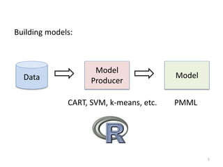
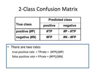
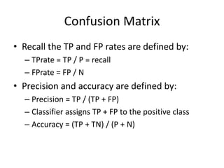
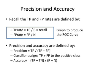
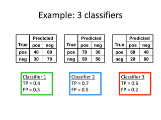
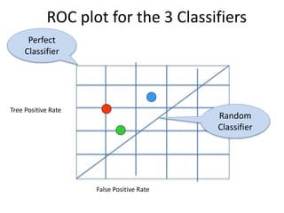
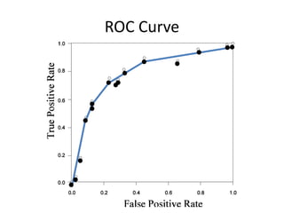
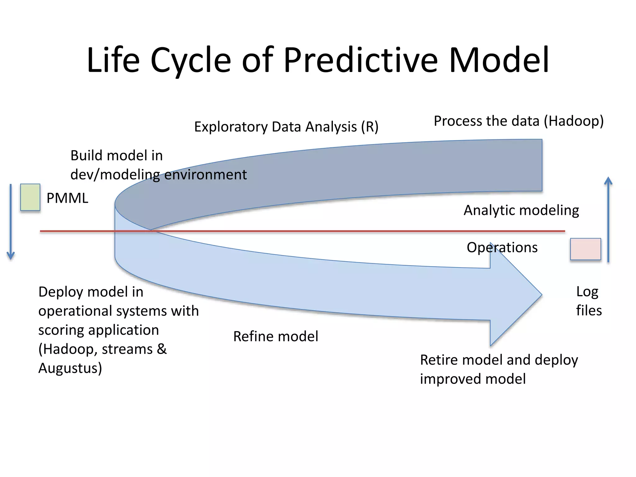
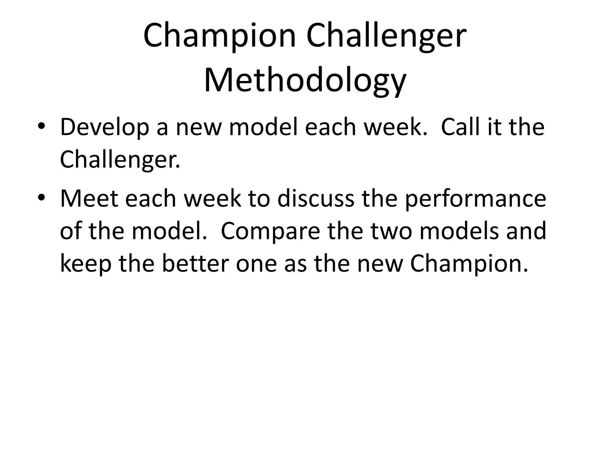
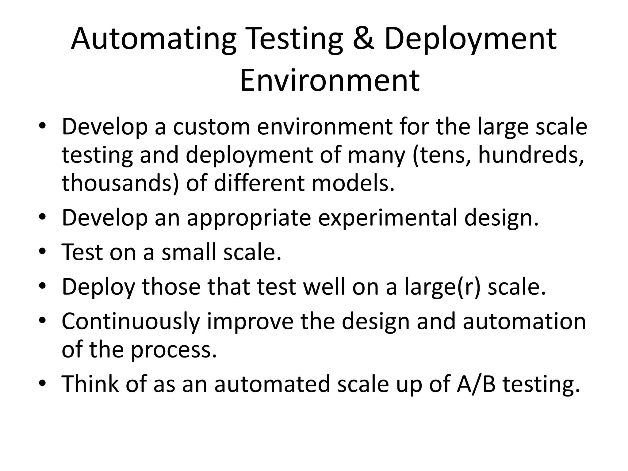
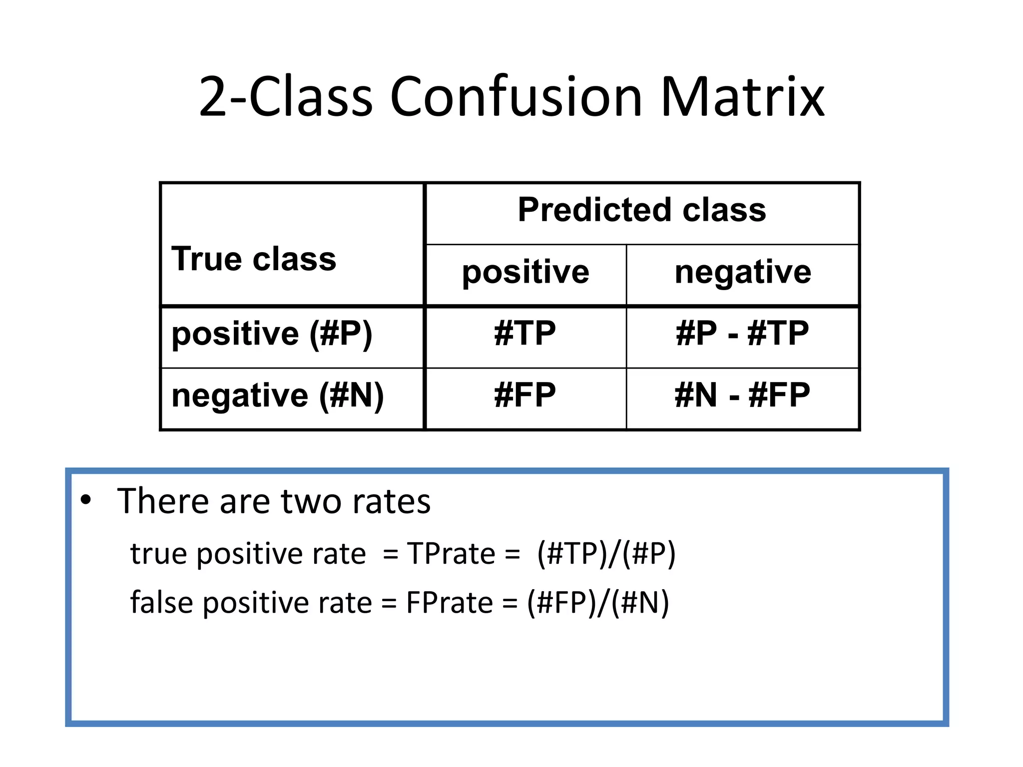
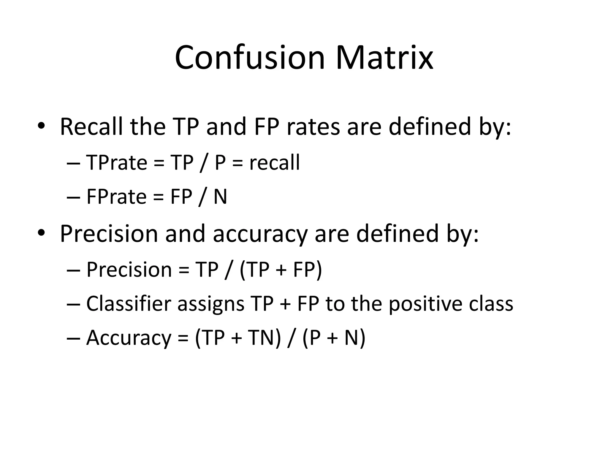
Robert Grossman and Collin Bennett of the Open Data Group discuss building and deploying big data analytic models. They describe the life cycle of a predictive model from exploratory data analysis to deployment and refinement. Key aspects include generating meaningful features from data, building and evaluating multiple models, and comparing models through techniques like confusion matrices and ROC curves to select the best performing model.


![Computing Count Distributions
def valueDistrib(b, field, select=None):
# given a dataframe b and an attribute field,
# returns the class distribution of the field
ccdict = {}
if select:
for i in select:
count = ccdict.get(b[i][field], 0)
ccdict[b[i][field]] = count + 1
else:
for i in range(len(b)):
count = ccdict.get(b[i][field], 0)
ccdict[b[i][field]] = count + 1
return ccdict](https://image.slidesharecdn.com/05-building-deploying-analytics-v2-170905012852/85/Building-and-deploying-analytics-17-320.jpg)
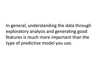
![Features
• Normalize
– [0, 1] or [-1, 1]
• Aggregate
• Discretize or bin
• Transform continuous to continuous or
discrete to discrete
• Compute ratios
• Use percentiles
• Use indicator variables](https://image.slidesharecdn.com/05-building-deploying-analytics-v2-170905012852/85/Building-and-deploying-analytics-18-320.jpg)


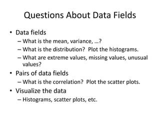
![Computing Count Distributions
def valueDistrib(b, field, select=None):
# given a dataframe b and an attribute field,
# returns the class distribution of the field
ccdict = {}
if select:
for i in select:
count = ccdict.get(b[i][field], 0)
ccdict[b[i][field]] = count + 1
else:
for i in range(len(b)):
count = ccdict.get(b[i][field], 0)
ccdict[b[i][field]] = count + 1
return ccdict](https://image.slidesharecdn.com/05-building-deploying-analytics-v2-170905012852/75/Building-and-deploying-analytics-17-2048.jpg)
![Features
• Normalize
– [0, 1] or [-1, 1]
• Aggregate
• Discretize or bin
• Transform continuous to continuous or
discrete to discrete
• Compute ratios
• Use percentiles
• Use indicator variables](https://image.slidesharecdn.com/05-building-deploying-analytics-v2-170905012852/75/Building-and-deploying-analytics-18-2048.jpg)


![[ppt]](https://cdn.slidesharecdn.com/ss_thumbnails/ppt2931-thumbnail.jpg?width=600ounds&width=560&fit=bounds)
![[ppt]](https://cdn.slidesharecdn.com/ss_thumbnails/ppt3441-thumbnail.jpg?width=600ounds&width=560&fit=bounds)


![Agentic Systems and Compliance - A brief intro [1.2]](https://cdn.slidesharecdn.com/ss_thumbnails/agenticsystemsandcompliace-1-251018025303-958a42ec-thumbnail.jpg?width=600ounds&width=560&fit=bounds)


![RTP_AR_Basic_Learners' Workbook_KS2 [FOR REPRODUCTION] (1).pdf](https://cdn.slidesharecdn.com/ss_thumbnails/rtparbasiclearnersworkbookks2forreproduction1-251016024943-e51a16ac-thumbnail.jpg?width=600ounds&width=560&fit=bounds)