Business Process Modeling
OnderwerpenMC II
Laguna, M. & Marklund, J. (2019 ). Business Process Modeling Simulation and Design
De volgende
onderwerpen
worden in deze les
behandeld:
(Her)ontwerp
proces
Framework voor
Business Process-
Design projecten
Gereedschappen
voor
procesbeschrijving
Geldende principes
voor
procesontwerp
4.
Business Process Modeling
OnderwerpenMC II
Laguna, M. & Marklund, J. (2019 ). Business Process Modeling Simulation and Design
Vorige keer I&II =>
definitie van:
Business process
Process design
Process management
Tacticts
Six sigma
BPM
Vandaag:
Framework voor “structuring business
process design projects”
Basis Tools for Process design
5.
Business Process Modeling
Laguna,M. & Marklund, J. (2019 ). Business Process Modeling Simulation and Design
The Overall Framework
• Step 1: Case for Action and Vision Statement
• Step 2: Process Identification and Selection
• Step 3: Obtain Management Commitment
• Step 4: Evaluate Design Enablers
• Step 5: Acquire Process Understanding
• Step 6: Creative Process Design
– Benchmarking
– Design Principles
• Step 7: Process Modeling and Simulation
• Step 8: Implementation of the New Process
Design
6.
A Simulation BasedFramework for
BPD Projects
1. Case for action
and vision
2. Process Identification
and selection
3. Obtaining Management
commitment
4. Evaluation of Design
Enablers
5. Acquiring Process
understanding
6. Creative Process
Design
7. Process Modeling and
Simulation
8. Implementation of the
New Process Design
Laguna, M. & Marklund, J. (2019 ). Business Process Modeling Simulation and Design
7.
A clearmessage about the need for change and where the
change is going to take us is necessary for successfully selling
the redesign concept to the company’s employees
Case for Action
– Here is where we are as a company and this is why we cannot stay here
– Five major elements build an effective argumentation
1. Business context – what is important and what is changing
2. Business problems – source of the company’s concern
3. Marketplace demand – performance standards & demands to
meet
4. Diagnostics – why are we unable to meet the posed demands
5. Cost of inaction – consequences of not changing
Case for Action and Vision Statements
(I)
Laguna, M. & Marklund, J. (2019 ). Business Process Modeling Simulation and Design
8.
• Process selectionis critical for the success of a design
project
– Core processes have the highest impact on overall performance
but are also more costly and risky to change
– The implementation tactic cannot be ignored, even due to
budget constraints
• Useful criteria for prioritization of projects are:
Dysfunction
Importance
Feasibility
• Other relevant screening issues/questions are:
What are the project’s scope and costs involved?
Can a strong and effective team be formed?
Is it likely to obtain strong management commitment?
Can other programs (e.g. continuous improvement) be used
instead?
Is the process obsolete or the technology outdated?
Process Identification and Selection
9.
• Top managementmust set the stage both for the design
project and the subsequent implementation
– Without top management support the improvement effort is bound
to fail
– The more profound and strategic the change is the more crucial the
top management support becomes
Obtaining Management Commitment
• Commitment assumes understanding
and cannot be achieved without
education
– People are more likely to be fearful and
resisting change if there is a lack of
direction and they do not understand the
implications of the change
– Occurrence of “resisting change” issues is
particularly prevalent in rapid revolutionary
change scenarios
10.
• New (information)technology is an essential
design enabler…
• …but could also reinforce old ways of thinking
– Automation redesign
– Do not look for problems first and then the
technology to fix them
– Evaluating new technology needs inductive thinking
• New technology should not be evaluated
within the structure of the existing process
– New technology enables us to break old rules and
compromises
• To avoid the automation trap the question to
ask is:
– How can new technology enable us to do new things
or to do things in new ways?
Evaluation of Design Enablers
11.
Technology as aMechanism to Break
Rules and Compromises
Old Rule New Technology New Rule
Information can appear Shared databases Information can appear
in only one place at a time. simultaneously in as many
places as needed.
Only experts can perform Expert systems A generalist may be able to do
complex work. the work of an expert.
The best contact with a potential Interactive videodisk The best contact with a potential
buyer is personal contact. and web pages. buyer is effective contact.
Businesses must choose Telecommunication Businesses can simultaneously
Between centralization networks reap the benefits of centralization
and decentralization.
and decentralization.
People must find where Automatic identification Things tell you where they are.
tracking technology. Plans get revised instantaneously.
things are.
Field personnel need offices Wireless data Field personnel can send and
Where to receive, store, retrieve
portable computers.
receive information wherever
and transmit information.
communication and
they are.
Plans get revised periodically. High performance
computers.
Plans get revised
instantaneously.
Managers make all decisions. (databases, modeling tools) everyone’s job.
Decision support tools -
Decision making is part of
12.
• Subtle differencebetween redesigning an existing
process and designing a new currently non-existing
process
– In both cases we need to understand the purpose of the
process and what the customers desire from it
– If the process exists, we need to understand what it is
currently doing and why it is unsatisfactory
• Business Process Benchmarking may be a useful
tool
– To gain process understanding
– To inspire creative new designs
Acquiring Process Understanding
13.
• Questions thedesign team needs to answer
What is the existing process doing?
How well does it perform?
What are the critical issues that impact the process performance?
• The redesign team must understand the process but should
not overanalyze it in order to avoid “analysis paralysis”
– Becoming so familiar with the process it is impossible to think of
new ways of doing it
• Essential activities for building process understanding
1. Configure the redesign team
2. Build a high level process map
3. Test the initial scope and scale
4. Identify the process owner
Understanding the Existing Process
14.
1. Configure theredesign team
– A mix of business insiders (managers and workers directly involved in
the current process) and business outsiders (consultants and employees
not involved in the process)
2. Build a high level process map
– Neither a low level flow chart nor an organizational chart
– Shows interactions between sub-processes, not the flow of data
– Focuses on customers and business outcomes
– Objectives
1. Build common understanding 4. Use a cross
functional vocabulary
2. Highlight critical sub-processes 5. Test initial scope
and scale
3. Identify key interfaces 6. Pinpoint redundancies and
waste
Activities for Building Process
Understanding (I)
15.
3. Test theinitial scope and scale
– Self examination
– Environmental
scanning/benchmarking
– Customer visits
4. Identify the process owner
– The person that will take
responsibility and be accountable for
the performance of the new process
Activities for Building Process
Understanding (II)
16.
Understanding the Customer
•The customer end is the best place to start
understanding a business process
– What are the customers’ real requirements?
– What do they say they need and what do they
really need?
– What problems do they have?
– What do they do with the process output?
• The ultimate goal with a business process
is to satisfy the customers’ real needs in an
efficient way!
17.
Creative Process Design(I)
• Designing new processes is more of an art than a
science
– Cannot be achieved through a formalized method
• Most existing processes were not designed; they just
emerged as new parts were added iteratively to
satisfy immediate needs
• The end result of any design is very much dependent
on the order in which information becomes available
– Inefficient processes are created when iterative design
methods are applied
18.
Illustration Process Evolution(I)
• Two pieces of plastic are given to you with instructions to
arrange them in an easily described shape
Illustration Process Evolution(III)
• Two more pieces are added, but very few people are
able to incorporate these and still obtain a simple shape
?
21.
Illustration Process Evolution(IV)
• Considering the pieces independently of the sequence
by which they appear leads to a much better solution!
22.
Benchmarking
• In thesame company, in the same industry or across industries
Comparing the firm’s/process’s activities and performance with what others are
doing
• The initiator firm – who initiates contact and observes (the pupil)
• The target firm (or benchmark) – who is being observed (the master)
Every benchmarking relationship involves two parties
Fruitful benchmarking relationships are usually characterized by reciprocity
• To assess the firm’s/process’s performance relative to the competition identify performance gaps and
goals
• To stimulate creativity and inspire innovative ideas for how to do things better, i.e. improve process
designs & process performance
Two basic benchmarking purposes
For BPD projects both purposes are relevant
23.
Design Principles
General people-orientedand conceptual process design principles
1. Organize work around
outcomes, not tasks
2. Let those who use the process
output perform the process
3. Merge information processing
and data gathering activities
5. Put the decision point where
the work is performed and build
control into the process
4. Capture the information once –
at the source
8. Design the process for the
dominant flow not the exceptions
6. Treat geographically dispersed
resources as though they were
centralized
7. Link parallel activities instead
of just integrating their output
9. Look for ways to mistake-proof
the process
10. Examine process interactions
to avoid sub-optimization
Themes:
Horizontal and vertical integration of
work, hand-off elimination, improved
quality and task coordination
Coordination of activities,
simplification of flows, elimination
of waste and rework
24.
1. Organize workaround outcomes not tasks
– Focus on horizontal integration of activities
– Eliminates unnecessary handoff and control steps
– Process complexity is reduced while activity complexity grows
• This integration approach often referred to as case management
2. Let those who use the process perform the process
– Work should be carried out where it makes most sense to do it
– Risk of coordination inefficiencies due to excessive delegation decreases
3. Merge information processing and data gathering
activities
– The people collecting the data should also process it into information
– Reduces the risk of errors and incorrect information
4. Capture information once – at the source
– Reduces costly reentry and frequency of erroneous data
– Speeds up the process, increases the quality of information and reduces
costs
Ten Conceptual Design Principles (I)
25.
5. Put thedecision point where the work is performed
and build control into the process
– Case management compresses processes horizontally and
employee empowerment compresses them vertically
– Workers are taking over previous management responsibilities
6. Treat geographically dispersed resources as though
they were centralized
– IT breaks spatial compromises through virtual co-location
– Geographically disbursed resources should not constrain the
design team to only consider decentralized approaches
7. Link/coordinate parallel activities instead of just
integrating their results
– If parallel activities are operated independently operational
errors are not detected until the outcomes are integrated
– Reduces the amount of rework
Ten Conceptual Design Principles (II)
26.
8. Design theprocess for the dominant flow not for
the exceptions
– Reduces the risk of fragmentation and overly complex
processes with inherent coordination problems
9. Look for ways to mistake-proof (or fail-safe) the
process
– Design so that certain critical errors cannot occur
– Mistake-proofing = Poke Yoke
10.Examining interactions to avoid sub-optimization
– By neglecting interactions, isolated improvements to sub-processes
will lead to sub-optimal solutions
– Known in systems theory as “disjointed incrementalism”
Ten Conceptual Design Principles (III)
27.
• Stems fromthe field of industrial engineering
– Successfully used for designing manufacturing systems for
decades
Seven Workflow Oriented Design
Principles
Establish product orientation in the process
Eliminate Buffers
Establish one at a time processing
Balance the flow to the bottleneck
Minimize sequential processing and hand-offs
Schedule work based on its critical characteristics
Minimize multiple paths due to specialized operations
for exception handling
Traditional, technically oriented workflow design principles
Focus: Efficient process flows, managing resource capacity,
throughput and cycle times
28.
• Conceptual processdesigns need to be tested before they are implemented in full
scale
– Pilot projects or process modeling techniques
• Business processes are often too complex and dynamic to be analyzed only with
simple tools like flowcharts and spreadsheets
• Discrete event simulation is a powerful and realistic tool to complement the more
simplistic methods
– Allows exploration of the redesign effects without costly interruptions of current operations
– Helps reduce the risks inherent in any design/change project
• Compared to pilot projects simulation is faster and cheaper
– Simulation not good for capturing soft people issues and attitudes
Simulation and pilots complement each other
Process Modeling and Simulation
29.
• A discreteevent simulation model mimics the
real world but in compressed time
– Focus only on events when the state of the system
changes and skips the time between these events
• Basic steps in evaluating a process design
through discrete event simulation
1. Building the simulation model
2. Running the simulation
3. Analyzing performance measures
4. Evaluation of alternative scenarios
Process Modeling and Simulation (II)
30.
Advantages with discreteevent simulation
• Promotes creativity by enabling easy testing of ideas
• Captures system dynamics but avoids disturbances
of current process
• Can capture interactions between sub-processes
– Mitigates the risk of sub-optimization
• Graphical reporting features promotes better process
understanding and facilitates communication
• The quantitative nature brings a sense of objectivity
into the picture
Process Modeling and Simulation (III)
31.
• Detailed implementationissues beyond the scope
of the design project
• High level implementation issues need to be
considered when selecting a process to design
– No point in designing a process which cannot be
implemented
• Crucial high level implementation issues
Time
Cost
Improvement potential
Likelihood of success
Implementation of the Process Design
(I)
32.
• Conceptually animplementation strategy can be
characterized as revolutionary, evolutionary or on
a continuum in between
– A rapid revolutionary approach tends to require more
external resources
• Regardless of the implementation tactic important
factors for a successful implementation are
Strong leadership
Buy-in from line managers and employees
Training of the workforce
Implementation of the Process Design
(II)
33.
• Important toreflect on what can be learned from a
given design and/or implementation project
– What worked, what didn’t and why?
– What were the main challenges?
– What design ideas didn’t work out in practice and why?
• The process of designing and implementing new
process designs also needs improvement
– Sharing experiences and collecting feedback is key to
any improvement effort
Final Notes
34.
In de vorigeles heb je een decompositie gemaakt wat de basis vormt
bij deze opdracht.
• Bespreek welke inzichten uit de de vorige les relevant zijn voor de
opzet van het kernproces.
• Vervaardig een model met de kernprocessen.
Opdracht Modelbouw
Groep van 2, 20 min
Deze opdracht is bedoeld om nogmaals stil te staan bij
het relevante processtappen, aangezien dit de
uitgangspunten zijn voor het ontwerp van het model
dat voor de simulatie wordt gebruikt.
35.
Overview
• Introduction BasicTools for BPD
• Graphical tools
– General Process Charts
– Process Activity Charts
– Process Flow Diagrams
– Flow Charts
– Service System Mapping
• Workflow Design Principles and Tools
– Establish product orientation in the process
– Eliminate buffers
– One-at-a-time processing
– Balancing bottleneck flows
– Minimize sequential processing and handoffs
– Scheduling based on job characteristics
– Minimize multiple paths
36.
• Deterministic toolsand modeling approaches to help
designers analyze processes and check proposed designs for
– Feasibility
– Completeness
– Efficiency
• Quantitative tools require data regarding important process
characteristics
– Steps required to complete the process
– Processing and activity times are key
• Tagging is an important technique for gathering process data
– Follow a job through the process
– Data is collected on a document (a tag) accompanying the job
– Particularly useful for gathering data on processing and activity
times
Basic Tools for Process Design
37.
• Summarizes thecurrent process the redesigned process
and the expected improvements
• Characterizes the process by
– The number of activities per category
– The amount of time spent in each activity category
– The percentage of the total processing time spent on each category
• Clearly indicates
– Major problems with the existing process
– How the redesigned process remedies these problems
• Problems measured in terms of the time and the percentage of
time spent on non-value adding activities
General Process Charts
38.
Illustration of aGeneral Process
Chart
Activities Current Process Redesigned Process
Difference
No. Time % No. Time % No.
Time
Operations 5 30 10 5 30 37.5 0 0
Inspections 3 60 20 1 20 25.0 -2 -
40
Transport. 10 120 40 2 20 25.0 -8 -
100
Storage 0 0 0 0 0 0 0 0
Delays 7 90 30 1 10 12.5 -6 -
80
Total 25 300 100 9 80 100 -16 -
39.
• Complements thegeneral process chart
– Provides details regarding the sequence of activities
• Disadvantages
– Only considers average activity times
– If the process includes several variants with different paths (i.e.
multiple paths through the process) each variant needs its own
activity chart
– Cannot depict parallel activities
Process Activity Charts
40.
Illustration of aProcess Activity Chart
Process Activity Chart
Process: __________________________
Developed by: ____________________
Page: ____ of _____
Date: __________
Current Process
Proposed Process
Description Time
Value code
(V/N/C) Symbol
No.
For each activity, fill in the required information. Also, connect
the symbols to show the flow through the process.
The value code indicates whether the activity adds value (V),
does not add value (N), or controls (C).
Adoption
1 6
9/14/99
X
1 Find where to go 2-10 N
2 Walk through 10-45 V
3 What’s next? 1-5 N
Operation
Inspection
Storage
Delay
Transportation of
a physical item
Symbols
41.
Je gaat insubgroepen aan het werk en vergelijkt je uitwerkingen van de voorbereidingsopdracht.
Ga tijdens het "modelleren in een gereedschap" met elkaar in gesprek.
Geef elkaar kritisch commentaar.
Ga hierbij na:
• Waarom welke techniek is gebruikt
• Wat de voor- en nadelen zijn van de verschillende technieken
• De juistheid en volledigheid van de toepassing.
• De duidelijkheid van de uitwerking met het oog op het beoogde doel.
Opdracht Modelleren in een gereedschap
Groep van 2, 20 min
Het doel van de opdracht is om inzicht te krijgen in de
verschillende modelleer methoden.
Wees kritisch bij het bepalen van de methode die je wilt
gebruiken.
Des te beter de methode aansluit bij het vraagstuk, des te
waardevoller zijn de resultaten uit het onderzoek.
Studenten vergelijken de uitwerkingen van de voorbereidingsopdracht Modelleren in een gereedschap
met elkaar
42.
• Provide apicture of the spatial relationships between
activities
– Typical application is for production floor layout problems.
• The diagram is used for measuring process performance in
units of time and distance
– Including both horizontal and vertical movements.
– Assumes that moving items requires a time proportional to the
distance.
• Can be used in conjunction with Process Activity Charts
– By labeling areas in the process flow diagram and by adding a
column to the activity chart, indicating for each activity which area
it belongs to.
– Alternatively, the flow diagram includes the activity numbers in
the activity chart.
Process Flow Diagrams (I)
43.
Illustration of aProcess Flow Diagram
C
B
A
F
E
D
Finished request
Incoming request
Before Redesign
C
B
A
F
E
Incoming request
Finished request
D
After Redesign
44.
• Analysis gearedtowards reducing excessive and
unnecessary transportation and movements of items/jobs
– Long distances
– Crisscrossing paths
– Repeated movements between the same activities
– Other illogical flows
• Can be used as a basis for computing Load Distance (LD)
scores
– Useful for quantitatively comparing alternative designs/layouts
with regards to flow rates and distances
Process Flow Diagrams (II)
45.
• LD(i,j) =LD score between work centers i and j
• The LD score measures the attraction between two work
centers (activities)
– The larger the traffic volume the higher the score and the higher
the incentive to keep the work centers together
• The goal is to find a design that minimizes the total LD
score (the sum of individual scores between work centers)
• The Load Matrix summarizes the load (flow rate = # of
jobs) that needs to be shipped between each pair of work
centers
Load Distance Analysis
LD(i,j) = Load(i,j)*Distance(i,j)
46.
A Sample LoadMatrix
A B C D E F
A 20 20 80
B 10 75
C 15 90
D 70
• See also example exercise on LD Analysis
47.
• One ofthe fundamental graphical tools for process
analysis and design
– Typically depicts activities sequentially from left to right
– Can help to identify, loops, multiple alternative paths, decision
points etc.
• Symbols often used in flow charting
Flow Charts
Transportation of a
physical item
Transportation of
information
Operation
Inspection
Storage
Delay
48.
Illustration of aSample Flow Chart
Operator
takes phone
order.
Orders wait
to be picked
up.
Supervisor
inspects
orders.
Order is
fulfilled.
Order waits
for sales rep.
Is order
complete?
Yes
No
Orders are
moved to
supervisor’s
in-box.
Orders
wait for
supervisor.
49.
• Flowcharts maybe used to estimate the total average process
time from the estimated activity times
– Assumes that the standard processing time is known (estimated)
– Assumes that the standard setup time is known (estimated)
– The standard times assumes 100% worker efficiency. If the worker is
less efficient the times must be adjusted as above.
Activity Times and Path Frequencies (I)
Average activity time =
(Unit processing time)*(batch size)+setup time
Efficiency
50.
Example: Inspection activity
•Inspection of one unit takes 3 minutes
• Each inspection batch includes 10 units
• It takes 15 minutes to prepare for the inspection of a batch
• The inspector is new on the job and it currently takes 25%
longer time to inspect a batch than when she is fully trained
What is the estimated activity time for inspecting a batch?
The average activity time = ((3*10) + 15)/0.75 = 60 minutes
Activity Times and Path Frequencies (II)
51.
• An extensionof traditional flowcharting
– Illustrates how effectively a business process satisfies customers across
all encounters
– Documents the role played by the customer in the service delivery
process
– A combination of service blue printing and traditional flowcharting
• Goals with SSM
– Build consistent perceptions of customer’s experience with core processes
– Identify all points of contact between the process and its customers
– Provide a basis for developing an economic business model
– Identify opportunities within the process
– Provide a design framework
– Aid in pinpointing control points and strategic performance measures
Service System Mapping (I)
52.
• An extensionof traditional flowcharting
– Illustrates how effectively a business process satisfies customers across all
encounters
– Documents the role played by the customer in the service delivery process
SSM Horizontal Bands
• The purpose is to organize activities according to the people or “players
in the process. – Who does what?
• A SSM typically consists of 5 bands
1. Customer band – end user
2. Frontline or distribution channel band
3. Back-room activity band
4. Centralized support or information systems band
5. Vendor or supplier band
SSM Process Segments
• A process segment or sub process is a set of activities that produces a
well defined output given some input
Service System Mapping
53.
Sample SSM foran Order Fulfillment
Process
Customer
Band
Front line
Band
Back-room
Band
IS
Band
Supplier
Band
Receiving Filling Shipping Billing
54.
• Software productsfor flowcharting and diagramming…
Micrografx PaceStar
RFFlow Visual Thought
SmartDraw TeamFlow
Tension Software Visio 2000
• A specialized approach for “enterprise modeling and
analysis” is the so called IDEF methodology
– A family of structured methods (functional, information and data
modeling)
– Based on an established graphical language SADT (Structured
Analysis and Design Technique)
– Used by many consulting firms not least in design of information
systems
Additional Diagramming Tools
55.
Organizing Activities
• Twobasic ways of organizing activities
1. By process (Process Orientation)
2. By product (Product Orientation)
• Process orientation (functional layout) groups activities or
workstations according to function
– Most common when the same activity is used for producing
different products or services or when serving many different
customers
– Utilization of equipment and personnel tends to be high
Workflow Design Principles and Tools (I)
56.
• Product orientationgroups all necessary activities to
complete a finished product into an integrated sequence of
work nodes or work stations
– A typical example is an assembly/production line for making a
particular car model
– Activities are organized around the route (needs) of a particular
product or service
– Advantages with product orientation include
• Faster processing rate
• Lower WIP
• Less unproductive time due to setups
• Less transportation time
• Less handoffs
– A capital intensive way of organizing activities
Workflow Design Principles and Tools (II)
57.
Product v.s. ProcessOrientation
1 2
4 5
3
Customer B
Customer A
(a)
1 2 4 5 3
3 1 4 2 5
Customer B
Customer A
(b)
Process Orientation Product Orientation
58.
• To justifya product orientation from a resource utilization
perspective the product/service volumes must be quite high.
• A popular hybrid between product and process orientation in
manufacturing is known as Group Technology (or product
clustering)
– Groups products with similar characteristics into families and
organizes activities around these families instead of around the
individual products
– “Product Family” orientation
• The equivalent in business processes would be to group jobs
with similar characteristics into families.
• The hybrid orientation simplifies customer routings, reduces
process time and can be justified even if the volumes of
individual products/services are not that large
A Hybrid Orientation
59.
Illustration of aHybrid Orientation
1
2 4 5
3
1
3
4 2 5
1
3
Customer C
Cell AC
Cell BD
Customer A
Customer B
Customer D
60.
Buffer Elimination
• Buffersare put in place to protect against variability in demand,
processing times, etc.
– Jobs stacked up at different parts of the process, waiting to be processed.
• WIP = Work In Process inventories.
– All jobs currently in the process, i.e. in queues/buffers, under
transportation or under processing.
• Buffers tend to cause logistical and communication problems
due to slower information feedback.
– Implies the need for advanced tracking systems to identify what job is in
which buffer.
• Product orientation implies less WIP but needs to be well
balanced in order to minimize buffers.
Workflow Design Principles and Tools (III)
61.
One-at-a-time Processing
• Reductionof the batch size to the size of one unit
• By reducing batch sizes (and setup times) the throughput
time and WIP can be minimized
• Two types of batches
1. Process batch
– All jobs being processed before the resource needs to be
changed to process jobs of a different kind
2. Transfer batch
– Number of items/jobs transported together to the next resource for
processing
– Usually the process batch
– By reducing the transfer batch total processing time and WIP are also
reduced
Workflow Design Principles and Tools (IV)
62.
• Three activitiesin
sequence 1, 2 & 3
• Processing times:
1 h/job in 1&3 and
0.5 h/job in
activity 2
• Consider the total
throughput time
for a batch of 100
units when the
transfer batch size
is: A) 100 B) 20
Example – Effect of Reducing Batch Sizes
1
2
3
Process
Batch
Transfer
Batch
100 100
100
100
100
100
100
50
100
250
100 20
20
20
20
100
20
130
1
2
3
Process
Batch
Transfer
Batch
63.
Balancing bottleneck flows
•Linked to the OM principle known as Theory of Constraints
(TOC) popularized by Eliyahu Goldrat in his book The Goal
– Balance flow not capacity!
– Keep bottlenecks fed!
• Historically manufacturers had tried to balance capacity
across processes to match market demands
– Making all activity capacities the same makes sense only if
processing times are constant or display marginal variability
– Variation in processing times causes inventory build up and idleness
at different parts of the process
• Only two ways of handling variation
– Increase WIP to smooth variation
– Differentiate/balance capacity according to the job flows
Workflow Design Principles and Tools (V)
64.
Line Balancing
• Auseful approach when processing times are fairly constant
– Should not be used when processing times display high variability
• The goal is to balance the capacity of the different workstations
constituting the production line (the process)
Procedure
1. Specify sequential (precedence) relationships among the
activities using a precedence diagram
2. Use market demand to determine the line’s desired cycle time per
work station (C)
Workflow Design Principles and Tools (VI)
C =
Process time per day
Market demand per day (in # of jobs)
65.
Line Balancing Procedure(continued)
3. Determine the theoretical minimum # of workstations (TM)
4. Select a primary rule to assign activities to workstations and a
secondary rule to break ties
5. Assign activities one at a time to workstation 1 as long as the
sum of activity times C. Repeat this for workstations 2,3, …
– Must satisfy the activities’ precedence relationships
6. Evaluate the line efficiency = Total process time/(C*#stations)
7. Rebalance using a different priority rule in case the efficiency is
unsatisfactory
Workflow Design Principles and Tools (VII)
TM =
Sum of activity times
C
66.
Potential Line BalancingComplications
• Market demand may require a work station
cycle time shorter than the longest activity time
Need to change the process in some way!
• Approaches:
– Split the activity
– Use parallel workstations
– Train the workers or upgrade machinery
for faster processing time
– Work overtime
– Redesign the entire process
Workflow Design Principles and Tools (VIII)
67.
Minimize Sequential Processingand Handoffs
• Sequential processing implies longer process throughput time
– Operations are dependent constrained by the slowest activity
– No one person is responsible for the entire service encounter
Illustrative example (see figure on next slide)
• A process with 4 activities, throughput time 30 minutes and
processing times 10, 7, 8 & 5 minutes in the 4 activities
• Sequential set up – each individual performs a different activity
– The process output is 60/10=6 jobs per hour
– The efficiency = (10+7+8+5)/(10*4) = 75%
• Parallel set up – each individual performs all 4 activities
– The process output is now 4*(60/30) = 8 jobs per hour
– The efficiency = 30/30 = 100%
Workflow Design Principles and Tools (IX)
68.
Illustrative Example –Sequential v.s.
Parallel Processing
30
min
30
min
30
min
30
min
Sequential processing
10
min
7
min
8
min
5
min
6 jobs/hour
Parallel processing
8 jobs/hour
69.
Scheduling based onjob characteristics (I)
• Scheduling involves sequencing the order at which a number of
different jobs are to pass through a workstation or process with
limited capacity
– Becomes more important as the diversity of jobs increases
• Characteristics that are commonly used as a basis for
scheduling
– Arrival time
– Estimated processing time
– Due date
– Importance
Workflow Design Principles and Tools (X)
70.
• Finding the“right”objective function and the best scheduling
characteristic to satisfy this objective is tricky
• Three common overall objectives
– Maximize process output over a given time period
– Satisfying customer desires for quality and promptness
– Minimizing current out-of-pocket costs
• Common surrogate objectives that are easier to quantify
– Minimize the makespan (the throughput time for a defined set of jobs)
– Minimize total (or average weighted ) tardiness (the time by which the
completion time surpasses the due date)
– Minimize the maximum tardiness
– Minimize the number of tardy jobs
• The weighted tardiness is obtained as the product between the
tardiness value and the importance weight of the job in question
Scheduling Based on Job Characteristics (II)
71.
• Commonly usedpriority rules are
– First-In-First-Out (FIFO) – scheduling according to arrival times
– Earliest-Due-Date first (EDD)
– Shortest Processing Time first (SPT)
(See example illustrating the application and effect of the different rules)
• Observations for a single server situation
– EDD render the optimal solution to the problem of minimizing the
maximum tardiness
– SPT render the schedule that minimizes the average throughput time
per job for a given set of jobs
Scheduling Based on Job Characteristics (III)
72.
Moore’s Algorithm
• Amethod for minimizing the number of tardy jobs, when all
jobs are considered equally important
1. Order the jobs according to the EDD rule.
2. Stop if no jobs are tardy – the optimal solution is found!
Go to step 6.
3. Find the first tardy job in the sequence.
4. Assuming that this tardy job is the kth
in the sequence. Find and
remove job j (j=1, 2, 3, …, k) with the longest processing time.
5. Revise the completion times and return to step 2
6. Insert the removed jobs at the end of the sequence in the order
they were removed
• See example illustrating the application of Moore’s algorithm
Scheduling Based on Job Characteristics (IV)
73.
Minimize the numberof multiple
paths through the process
• Reduces complexity and confusion
– Simplifies resource management and
scheduling
– Fewer jobs are routed the wrong path and need
to be rerouted or reworked
Workflow Design Principles and Tools (XI)
• One way of reducing the number of paths without
compromising the efficiency and customization ability is to
use case teams, i.e., horizontal compression of work flow
74.
Dado Cukor
Lecturer ofInnovation & Strategic Management
Member of board of examiners (Master & Bachelor)
NCOI Business School
d.cukor@gmail.com
www.linkedin.com/in/cukor
+31 6 5160 36 88
Bedankt
Slides are available: e-connect
Think Free & don’t forget a Fun
Voorbereiding:
• Modelbouw
• Modelleren in een gereedschap
75.
Business Process Modeling
Dataverzameling
Laguna, M. & Marklund, J. (2019 ). Business Process Modeling Simulation and Design
In deze les wordt ingegaan op het verzamelen van gegevens, die van
belang zijn voor het management van proces-flows. Ook wordt uitvoerig
ingegaan op het modelleren van wachtrijen. Hiermee wordt inzicht
ontwikkeld in de meer mathematische aanpak bij het bestuderen van
wachtrijsituaties.
Analyse van de
capaciteit
Cycle time
Beslissingsmodellen
bij wachtrijen
Theory of
Constraints (TOC)
Gegevens
verzamelen
Problemen bij het
verzamelen van
gegevens
76.
1. Id en tify a
p ro b le m
3. M a ke
d e c is io n s
2 . An alys e th e
p ro b le m
4 . Im p le m e n t
th e d e cisio n s
B u ild a m o d e l
an d te s t it
An alyse th e
re su lts
Stu d y th e
d e ta ils o f th e
p ro b le m
Te st th e m o d e l
an d d a ta
Id e n tify ke y
v ariab le s an d
re la tio n s h ip s
b e tw e e n th e m
C o lle ct an d
a n alyse d ata
Ex p e rim e n t w ith
th e m o d e l an d
g e t re su lts
Solving a problem
Q u alita tiv e
an alyse s
Q u a n titativ e
a n a lyse s
M odelling
Figure 1.3 The role of modelling in solving a problems
C h e ck p re v io u s
w o rk
C o n s id e r
d iffe re n t
ap p ro a ch e s
77.
Overview
• Processes andFlows – Important Concepts
– Throughput
– WIP
– Cycle Time
– Little’s Formula
• Cycle Time Analysis
• Capacity Analysis
• Managing Cycle Time and Capacity
– Cycle time reduction
– Increasing Process Capacity
• Theory of Constraints
78.
A process =A set of activities that transforms inputs to outputs
Two main methods for processing jobs
1. Discrete – Identifiable products or services
Examples: Cars, cell phones, clothes etc.
2. Continuous – Products and services not in identifiable distinct units
Examples: Gasoline, electricity, paper etc.
• Three main types of flow structures
1. Divergent – Several outputs derived from one input
Example: Dairy and oil products
2. Convergent – Several inputs put together to one output
Example: Car manufacturing, general assembly lines
3. Linear – One input gives one output
Example: Hospital treatment
Processes and Flows – Concepts
79.
• Inflow andOutflow rates typically vary over time
– IN(t) = Arrival/Inflow rate of jobs at time t
– OUT(t) = Departure/Outflow rate of finished jobs at time t
– IN = Average inflow rate over time
– OUT = Average outflow rate over time
• A stable system must have IN=OUT=
– = the process flow rate
– = process throughput
Process Throughput
80.
0
2
4
6
8
10
12
1 3 57 9 11 13 15 17 19 21 23 25 27 29
t
Jobs
IN(t)
OUT(t)
Process Inflow and Outflow vary over
time
81.
• All jobsthat have entered the process but not yet left it
• A long lasting trend in manufacturing has been to lower WIP by
reducing batch sizes
– The JIT philosophy
– Forces reduction in set up times and set up costs
• WIP = Average work in process over time
• WIP(t) = Work in process at time t
– WIP(t) increases when IN(t)>OUT(t)
– WIP(t) decreases when IN(t)<OUT(t)
Work-In-Process
82.
The WIP LevelVaries With
Process Inflow and Outflow
t1 t2 t3
WIP(t)
WIP
OUT(t) > IN(t)
IN(t) > OUT(t)
OUT(t) = IN(t)
83.
The difference betweena job’s departure time and its arrival time = cycle time
• One of the most important attributes of a process
• Also referred to as throughput time
The cycle time includes both value adding and non-value adding activity times
• Processing time
• Inspection time
• Transportation time
• Storage time
• Waiting time
Cycle time is a powerful tool for identifying process improvement potential
Process Cycle Time
84.
• States afundamental and very general relationship between the
average: WIP, Throughput (= ) and Cycle time (CT)
– The cycle time refers to the time the job spends in the system or process
• Implications, everything else equal
– Shorter cycle time lower WIP
– If increases to keep WIP at current levels CT must be reduced
• A related measure is (inventory) turnover ratio
– Indicates how often the WIP is entirely replaced by a new set of jobs
Little’s Formula
(Due to J.D.C. Little (1961))
Little’s Formula: WIP = ·CT
Turnover ratio = 1/CT
• The taskof calculating the average cycle time for an entire process or
process segment:
– Assumes that the average activity times for all involved activities are available
• In the simplest case a process consists of a sequence of activities on a
single path
– The average cycle time is just the sum of the average activity times involved
• … but in general we must be able to account for
– Rework
– Multiple paths
– Parallel activities
Cycle Time Analysis
87.
• Many processesinclude control or inspection points where
if the job does not conform it will be sent back for rework
– The rework will directly affect the average cycle time!
• Definitions
– T = sum of activity times in the rework loop
– r = percentage of jobs requiring rework (rejection rate)
• Assuming a job is never reworked more than once
• Assuming a reworked job is no different than a regular job
Rework
CT = (1+r)T
CT = T/(1-r)
88.
Example – Reworkeffects on the
average cycle time
• Consider a process consisting of
– Three activities, A, B & C taking on average 10 min. each
– One inspection activity (I) taking 4 minutes to complete.
– X% of the jobs are rejected at inspection and sent for rework
What is the average cycle time?
a) If no jobs are rejected and sent for rework.
b) If 25% of the jobs need rework but never more than once.
c) If 25% of the jobs need rework but reworked jobs are no different in
quality than ordinary jobs.
0.75
0.25
A
(10)
B
(10)
C
(10)
I
(4)
89.
• It iscommon that there are alternative routes through the process
– For example: jobs can be split in “fast track”and normal jobs
• Assume that m different paths originate from a decision point
– pi = The probability that a job is routed to path i
– Ti = The time to go down path i
Multiple Paths
CT = p1T1+p2T2+…+pmTm=
m
1
i
i
iT
p
90.
Example – Processeswith Multiple
Paths
• Consider a process segment consisting of 3 activities A, B & C with activity times 10,15 & 20 minutes
respectively
• On average 20% of the jobs are routed via B and 80% go straight to activity C.
What is the average cycle time?
0.8
0.2
A
(10)
B
(15)
C
(20)
91.
• If twoactivities related to the same job are done in parallel
the contribution to the cycle time for the job is the
maximum of the two activity times.
• Assuming
– M process segments in parallel
– Ti = Average process time for process segment i to be completed
Processes with Parallel Activities
CTparallel = Max{T1, T2,…, TM}
92.
• Consider aprocess segment with 5 activities A, B, C, D & E
with average activity times: 12, 14, 20, 18 & 15 minutes
What is the average cycle time for the process segment?
Example – Cycle Time Analysis of
Parallel Activities
A
(12)
B
(14)
C
(20)
D
(18)
E
(15)
93.
Lesopdracht: Berekenen vangemiddelde en
variantie. Gr van 3. 20 min
Inleiding docent
Studenten gaan in groepjes van 3-4 personen om hun bevindingen met elkaar te delen
betreffende het verkrijgen van de data bij de ICT dienst.
Bespreek plenair de verschillende grafieken en tabellen.
Ga daarbij in op de verschillen in data binnen een proces:
• zoals de verschillen in omvang,
• tijdsduur,
• aantallen (klanten en producten), etc.
De bevindingen wordt met elkaar gedeeld in de les om het inzicht te verbeteren in de
wiskundige benadering.
94.
• Measured asthe percentage of the total cycle time spent on value adding activities.
• Theoretical Cycle Time = the cycle time which we would have if only value adding
activities were performed
– That is if the activity times, which include waiting times, are replaced by the processing times
Cycle Time Efficiency
Cycle Time Efficiency =
CT
Time
Cycle
l
Theoretica
95.
• Focus onassessing the capacity needs and resource utilization in the
process
1. Determine the number of jobs flowing through different process segments
2. Determine capacity requirements and utilization based on the flows obtained in 1.
• The capacity requirements are directly affected by the process
configuration
Þ Flowcharts are valuable tools
Þ Special features to watch out for
Rework
Multiple Paths
Parallel Activities
• Complements the cycle time analysis!
Capacity Analysis
96.
• A reworkloop implies an increase of the flow rate for that
process segment
• Definitions
– N = Number of jobs flowing through the rework loop
– n = Number of jobs arriving to the rework loop from other
parts of the process
– r = Probability that a job needs rework
• Assuming a job is never reworked more than once
• Assuming a reworked job is no different than a regular job
The Effect of Rework on Process Flows
N = (1+r)n
N = n/(1-r)
97.
N = (1+r)n= (1+0.25)100 = 125
Example – Capacity Analysis with Rework
0.75
0.25
A B C I
100 jobs 125 jobs 125 jobs 125 jobs
98.
Multiple Paths andprocess flows
• The flow along a certain path depends on
– The number of jobs entering the process as a whole (n)
– The probability for a job to go along a certain path
• Defining
– Ni = number of jobs taking path i
– pi = Probability that a job goes along path i
Parallel Activities and process flows
• All jobs still have to go through all activities
– if they are in parallel or sequential does not affect the number of
jobs flowing through a particular activity
Multiple Paths and Parallel Activities
Ni = n·pi
99.
Need toknow
– Processing times for all activities
– The type of resource required to perform the activity
– The number of jobs flowing through each activity
– The number of available resources of each type
Step 1 – Calculate unit load for each resource
• The total resource time required to process one job
– Ni = Number of jobs flowing through activity i for every new job entering the process
– Ti = The processing time for activity i in the current resource
– M = Total number of activities using the resource
Analyzing Capacity Needs and Utilization
Unit load for resource j =
M
1
i
i
i T
N
100.
Step 2 –Calculate the unit capacity
• The number of jobs per time unit that can be processed
Step 3 – Determine the resource pool capacity
• A resource pool is a set of identical resources available for use
• Pool capacity is the number of jobs per time unit that can be processed
– Let M = Number of resources in the pool
Analyzing Capacity Needs and Utilization
Unit capacity for resource j = 1/Unit load for resource j
Pool capacity = MUnit capacity = M/unit load
101.
Capacity isrelated to resources not to activities!
• The process capacity is determined by the bottleneck
– The bottleneck is the resource or resource pool with the smallest capacity (the
slowest resource in terms of jobs/time unit)
– The slowest resource will limit the process throughput
Capacity Utilization
• The theoretical process capacity is obtained by focusing on processing
times as opposed to activity times
– Delays and waiting times are disregarded
ÞThe actual process throughput The theoretical capacity!
Analyzing Capacity Needs and Utilization
Capacity Utilization =
Capacity
ocess
Pr
l
Theoretica
Throughput
Actual
102.
Cycle timeand capacity analysis provide valuable information about
process performance
– Helps identify problems
– Increases process understanding
– Useful for assessing the effect of design changes
• Ways of reducing cycle times through process redesign
1. Eliminate activities
2. Reduce waiting and processing time
3. Eliminate rework
4. Perform activities in parallel
5. Move processing time to activities not on the critical path
6. Reduce setup times and enable batch size reduction
Cycle time Reduction
103.
• Consider aprocess with three sequences or paths
Þ By moving 2 minutes of activity time from path 2 to path 1 the cycle
time is reduced by 2 minutes to CT=45 minutes
Example – Critical Activity Reduction
A
B
C
D
E
12 1
5
18
20
14
Sequence (Path) Time required (minutes)
1. AB E 12+14+15 = 41
2. AC E 12+20+15 = 47 = CT
3. A D E 12+18+15 = 45
Critical path
104.
• Two fundamentalways of increasing process capacity
1. Add resource capacity at the bottleneck
– Additional equipment, labor or overtime
– Automation
2. Reduce bottleneck workload
– Process redesign
Shifting activities from the bottleneck to other resources
Reducing activity time for bottleneck jobs
• When the goal is to reduce cycle time and increase
capacity careful attention must be given to
– The resource availability
– The assignment of activities to resources
• See also example 5.15 in Laguna & Marklund
Increasing Process Capacity
105.
• An approachfor identifying and managing bottlenecks
– To increase process flow and thereby process efficiency
• TOC is focusing on improving the bottom line through
– Increasing throughput
– Reducing inventory
– Reducing operating costs
Þ Need operating policies that move the variables in the right directions
without violating the given constraints
• Three broad constraint categories
1. Resource constraints
2. Market constraints
3. Policy constraints
Theory of Constraints (TOC)
106.
• TOC Methodology
1.Identify the system’s constraints
2. Determine how to exploit the constraints
– Choose decision/ranking rules for processing jobs in bottleneck
3. Subordinate everything to the decisions in step 2
4. Elevate the constraints to improve performance
– For example, increasing bottleneck capacity through investments in
new equipment or labor
5. If the current constraints are eliminated return to step 1
– Don’t loose inertia, continuous improvement is necessary!
• See example 5.18 , Chapter 5 in Laguna & Marklund
Theory of Constraints (TOC)
107.
• Consider aprocess with 9 activities and three resource types.
Activities 1, 2 & 3 require 10 minutes of processing and the
other activities 5 minutes each.
• There are 3 jobs, following different paths being processed
• Activities 1, 2 & 3 utilize resource X, activities 4, 5, & 6
resource Y and activities 7, 8 & 9 resource Z. Each resource
have 2400 minutes of weekly processing time available
Example – Applying the TOC Methodology
Job Routing Demand
(Units/week)
Profit Margin
A 4, 8, and 9 50 20
B
1, 2, 3, 5, 6,
7, and 8
100 75
C
2, 3, 4, 5, 6,
7, 8, and 9
60 60
108.
What is QueuingTheory?
• Mathematical analysis of queues and waiting
times in stochastic systems.
– Used extensively to analyze production and
service processes exhibiting random
variability in market demand (arrival
times) and service times.
• Queues arise when the short term demand for
service exceeds the capacity
– Most often caused by random variation in
service times and the times between
customer arrivals.
– If long term demand for service > capacity
the queue will explode!
108
109.
• Capacity problemsare very common in industry and one of the main
drivers of process redesign
– Need to balance the cost of increased capacity against the gains of increased
productivity and service
• Queuing and waiting time analysis is particularly important in service
systems
– Large costs of waiting and of lost sales due to waiting
Prototype Example – ER at County Hospital
• Patients arrive by ambulance or by their own accord
• One doctor is always on duty
• More and more patients seeks help longer waiting times
Question: Should another MD position be instated?
Why is Queuing Analysis
Important?
• Commercial QueuingSystems
– Commercial organizations serving external customers
– Ex. Dentist, bank, ATM, gas stations, plumber, garage …
• Transportation service systems
– Vehicles are customers or servers
– Ex. Vehicles waiting at toll stations and traffic lights, trucks or ships
waiting to be loaded, taxi cabs, fire engines, elevators, buses …
• Business-internal service systems
– Customers receiving service are internal to the organization providing
the service
– Ex. Inspection stations, conveyor belts, computer support …
• Social service systems
– Ex. Judicial process, the ER at a hospital, waiting lists for organ
transplants or student dorm rooms …
Examples of Real World Queuing Systems?
112.
Components of aBasic Queuing
Process
Calling
Population
Queue
Service
Mechanism
Input Source The Queuing System
Jobs
Arrival
Process
Queue
Configuration
Queue
Discipline
Served
Jobs
Service
Process
leave the
system
113.
The callingpopulation
– The population from which customers/jobs originate
– The size can be finite or infinite (the latter is most common)
– Can be homogeneous (only one type of customers/ jobs) or
heterogeneous (several different kinds of customers/jobs)
The Arrival Process
– Determines how, when and where customer/jobs arrive to the system
– Important characteristic is the customers’/jobs’ inter-arrival times
– To correctly specify the arrival process requires data collection of
interarrival times and statistical analysis.
Components of a Basic Queuing
Process
114.
The queueconfiguration
– Specifies the number of queues
• Single or multiple lines to a number of service stations
– Their location
– Their effect on customer behavior
• Balking and reneging
– Their maximum size (# of jobs the queue can hold)
• Distinction between infinite and finite capacity
Components of a Basic Queuing
Process
115.
Example – TwoQueue Configurations
Servers
Multiple Queues
Servers
Single Queue
116.
1. The serviceprovided can be
differentiated
– Ex. Supermarket express lanes
2. Labor specialization possible
3. Customer has more flexibility
4. Balking behavior may be
deterred
– Several medium-length lines
are less intimidating than one
very long line
1. Guarantees fairness
– FIFO applied to all arrivals
2. No customer anxiety
regarding choice of queue
3. Avoids “cutting in” problems
4. The most efficient set up for
minimizing time in the queue
5. Jockeying (line switching) is
avoided
Multiple v.s. Single Customer Queue
Configuration
Multiple Line
Advantages
Single Line Advantages
117.
A Commonly SeenQueuing Model (I)
C C C … C
Customers (C)
C S = Server
C S
•
•
•
C S
Customer =C
The Queuing System
The Queue
The Service Facility
118.
• Service timesas well as interarrival times are assumed independent and
identically distributed
– If not otherwise specified
• Commonly used notation principle: A/B/C
– A = The interarrival time distribution
– B = The service time distribution
– C = The number of parallel servers
• Commonly used distributions
– M = Markovian (exponential) - Memoryless
– D = Deterministic distribution
– G = General distribution
• Example: M/M/c
– Queuing system with exponentially distributed service and inter-arrival times and c servers
A Commonly Seen Queuing Model
119.
The most commonlyused queuing models are based on the
assumption of exponentially distributed service times and
interarrival times.
Definition: A stochastic (or random) variable Texp( ),
i.e., is exponentially distributed with parameter , if its
frequency function is:
The Exponential Distribution and
Queuing
0
t
when
0
0
t
when
e
)
t
(
f
t
T
t
T e
1
)
t
(
F
The Cumulative Distribution Function is:
The mean = E[T] = 1/
The Variance = Var[T] = 1/ 2
Stochastisch = De aanwezigheid
van een toevalsvariabele.
Een stochastisch proces houdt in dat
het systeem een element van toeval
kent (bijvoorbeeld merkenwissel
wordt vaak als
een stochastisch proces gezien).
T = random variabele representing
either interarrival times or services
times in a queuing proces.
Relationship tothe Poisson distribution and the Poisson Process
Let X(t) be the number of events occurring in the interval
[0,t]. If the time between consecutive events is T and
Texp()
X(t)Po(t) {X(t), t0} constitutes a Poisson Process
Properties of the Exp-distribution (IV)
...
,
1
,
0
n
for
!
n
e
)
t
(
)
n
)
t
(
X
(
P
nt
n
122.
Definition: Astochastic process in continuous time is a family
{X(t)} of stochastic variables defined over a continuous set of
t-values.
• Example: The number of phone calls connected through a
switch board
Definition: A stochastic process {X(t)} is said to have
independent increments if for all disjoint intervals (ti, ti+hi) the
differences Xi(ti+hi)Xi(ti) are mutually independent.
Stochastic Processes in Continuous
Time
X(t)=# Calls
t
123.
The standardassumption in many queuing models is that the
arrival process is Poisson
Two equivalent definitions of the Poisson Process
1. The times between arrivals are independent, identically
distributed and exponential
2. X(t) is a Poisson process with arrival rate iff.
a) X(t) have independent increments
b) For a small time interval h it holds that
P(exactly 1 event occurs in the interval [t, t+h]) = h + o(h)
P(more than 1 event occurs in the interval [t, t+h]) = o(h)
The Poisson Process
124.
Illustration – Disaggregatinga
Poisson Process
X(t)Po(t)
)
t
(
Po
)
t
p
(
Po
)
t
(
X 1
1
1
)
t
(
Po
)
t
p
(
Po
)
t
(
X 2
2
2
)
t
(
Po
)
t
p
(
Po
)
t
(
X N
N
N
p1
p2
pN
125.
The stateof the system = the number of customers in the system
Queue length = (The state of the system) – (number of customers being served)
N(t) = Number of customers/jobs in the system at time t
Pn(t) = The probability that at time t, there are n customers/jobs in the system.
n = Average arrival intensity (= # arrivals per time unit) at n customers/jobs
in the system
n = Average service intensity for the system when there are n customers/jobs
in it.
(Note, the total service intensity for all occupied servers)
= The utilization factor for the service facility.
(= The expected fraction of the time that the service facility is being used)
Terminology and Notation
126.
Example – ServiceUtilization Factor
• Consider an M/M/1 queue with arrival rate = and service intensity =
• = Expected capacity demand per time unit
• = Expected capacity per time unit
μ
λ
Capacity
Available
Demand
Capacity
ρ
*
c
Capacity
Available
Demand
Capacity
• Similarly if there are c servers in parallel, i.e., an M/M/c system
but the expected capacity per time unit is then c*
127.
• Steady Statecondition
– Enough time has passed for the system state to be independent of the
initial state as well as the elapsed time
– The probability distribution of the state of the system remains the same
over time (is stationary).
• Transient condition
– Prevalent when a queuing system has recently begun operations
– The state of the system is greatly affected by the initial state and by the
time elapsed since operations started
– The probability distribution of the state of the system changes with
time
Queuing Theory Focus on Steady
State
With few exceptions Queuing Theory has focused on analyzing
steady state behavior
128.
Transient and SteadyState Conditions
• Illustration of transient and steady-state conditions
– N(t) = number of customers in the system at time t,
– E[N(t)] = represents the expected number of customers in the system.
Transient condition
0
5
10
15
20
25
30
0 5 10 15 20 25 30 35 40 45 50
time, t
Number
of
jobs
in
the
system,
N(t)
Steady State condition
E[N(t)]
N(t)
129.
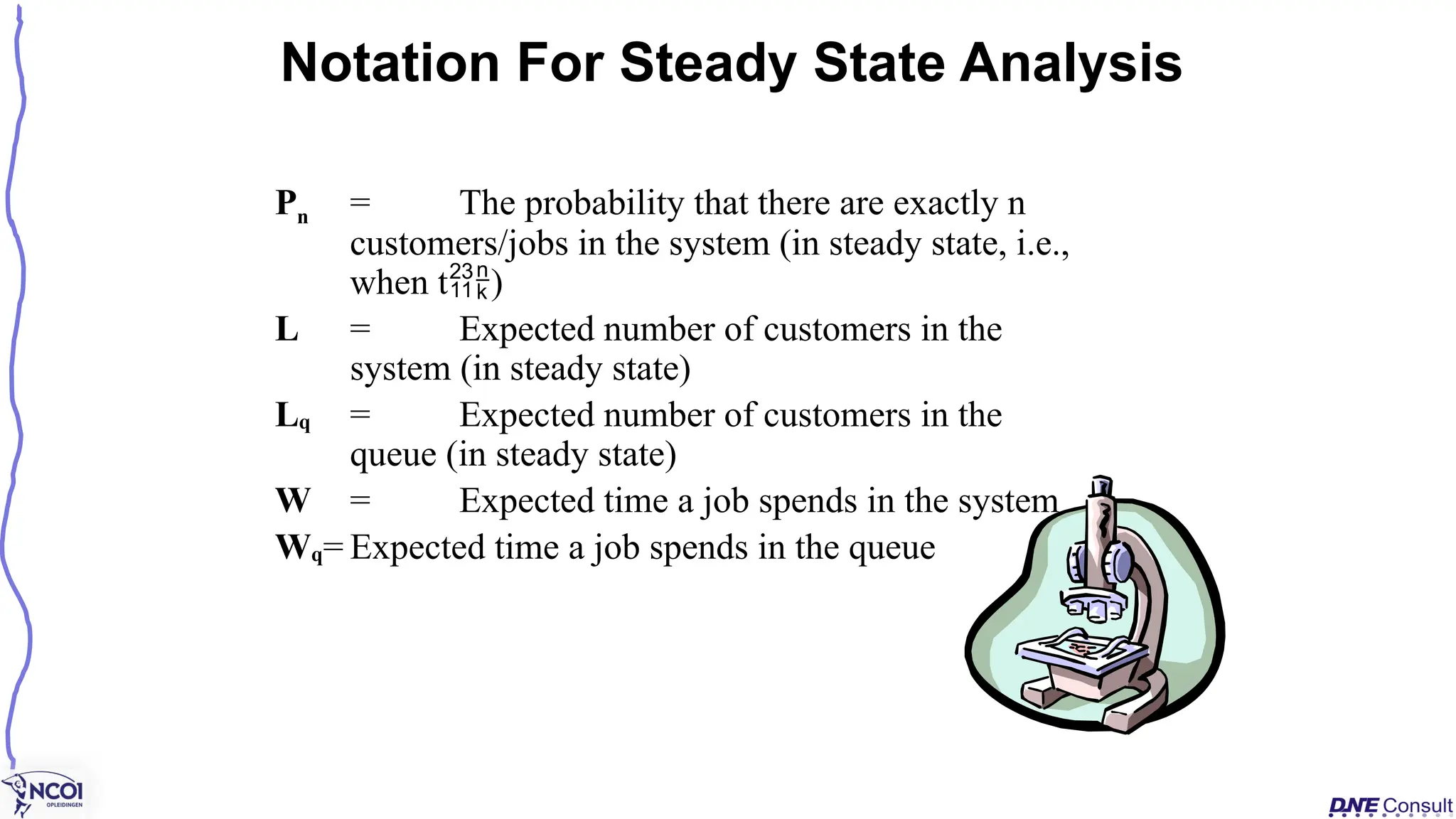
Pn = Theprobability that there are exactly n
customers/jobs in the system (in steady state, i.e.,
when t)
L = Expected number of customers in the
system (in steady state)
Lq = Expected number of customers in the
queue (in steady state)
W = Expected time a job spends in the system
Wq= Expected time a job spends in the queue
Notation For Steady State Analysis
130.
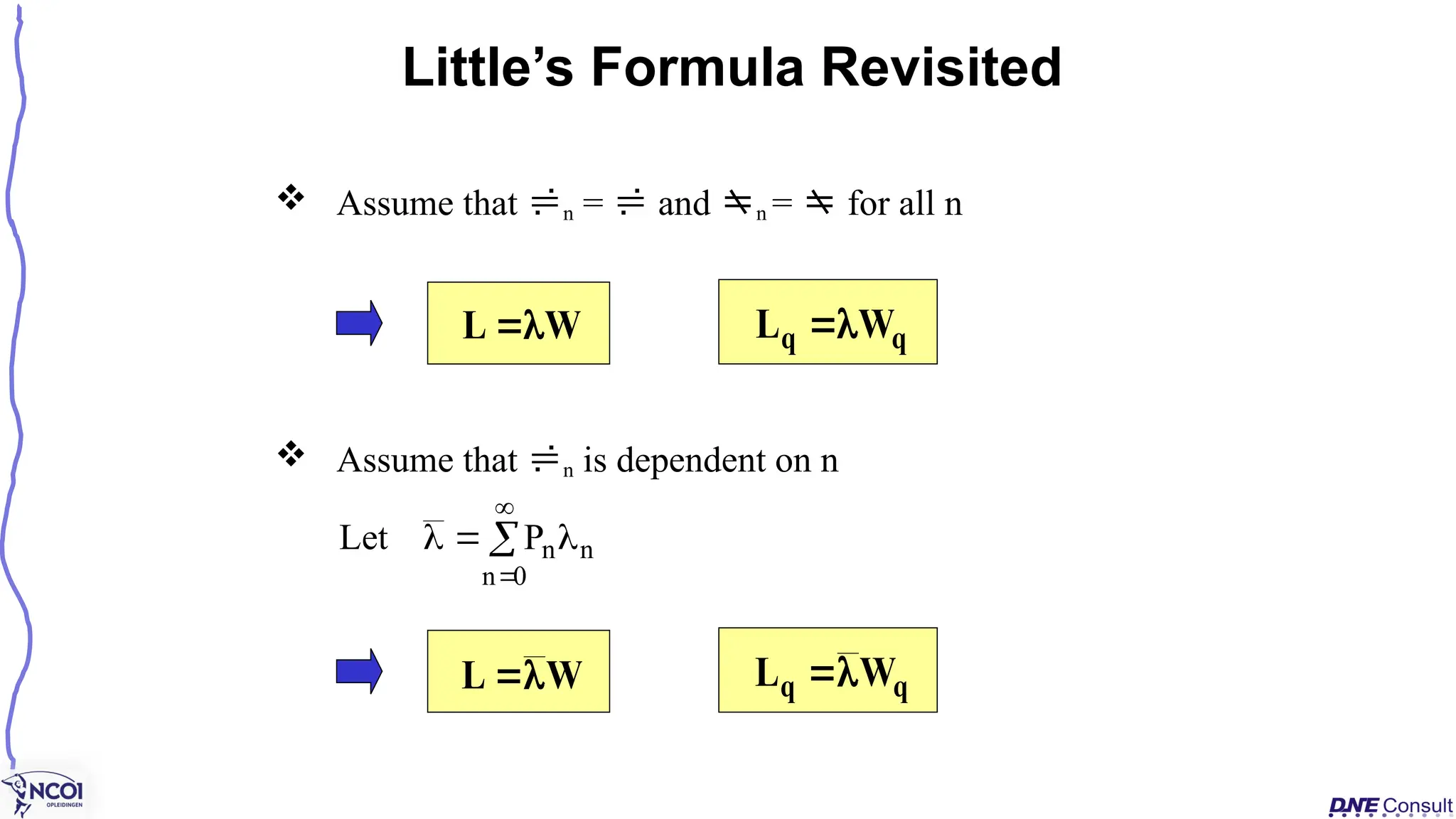
Assume thatn = and n = for all n
Assume that n is dependent on n
Little’s Formula Revisited
W
L
q
q W
L
W
L
q
q W
L
0
n
n
n
P
Let
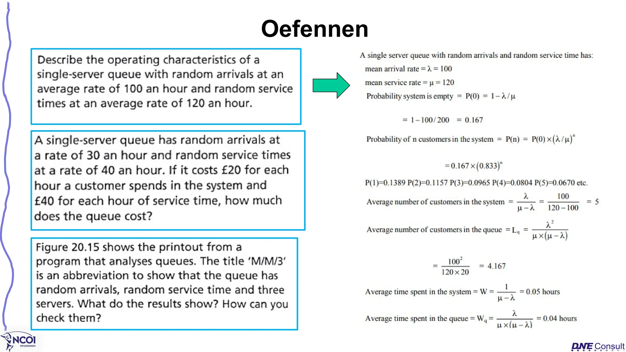
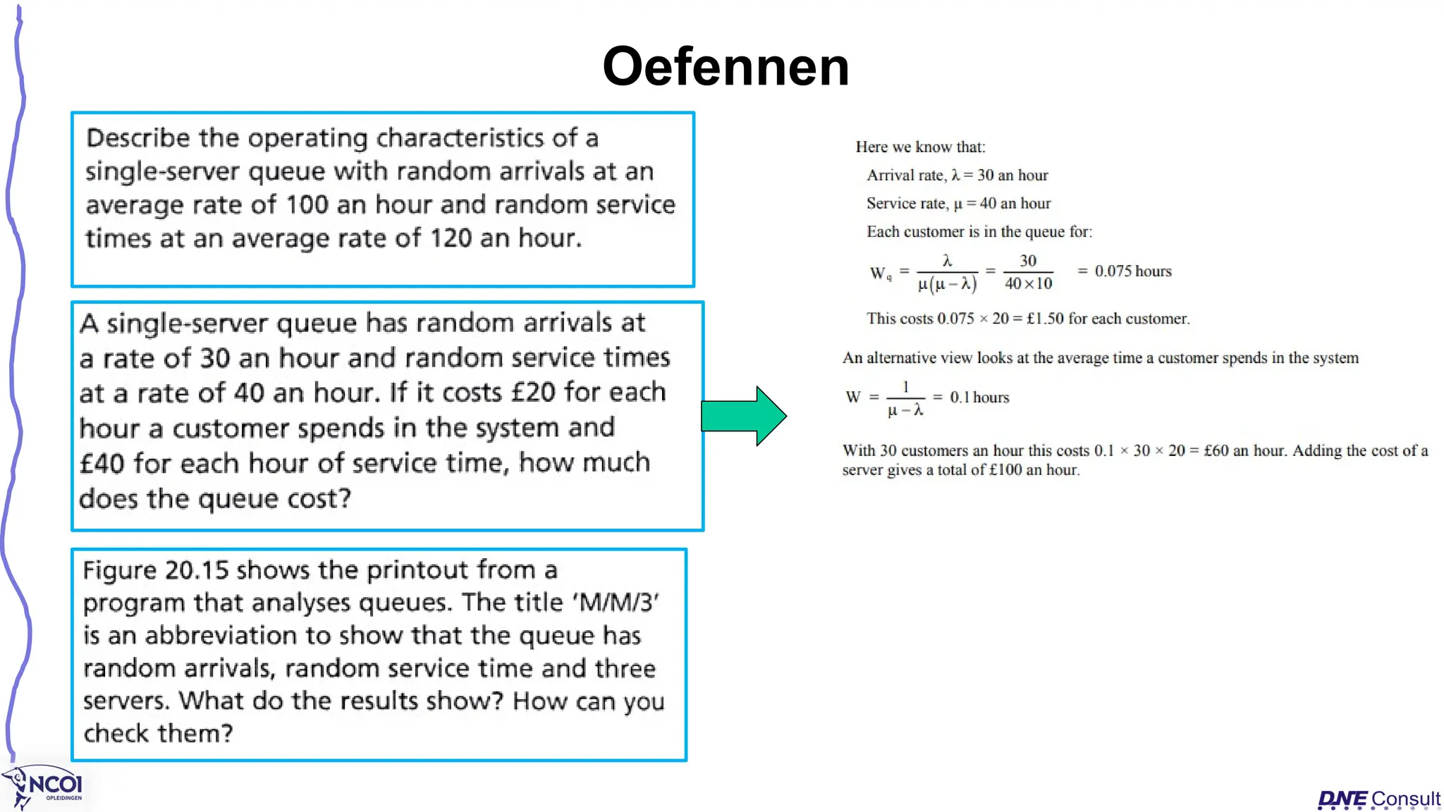
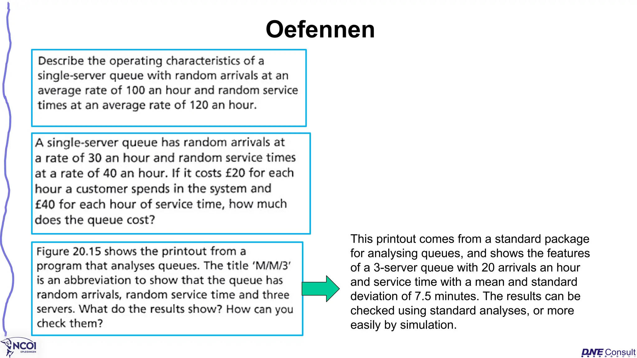
Oefennen
This printout comesfrom a standard package
for analysing queues, and shows the features
of a 3-server queue with 20 arrivals an hour
and service time with a mean and standard
deviation of 7.5 minutes. The results can be
checked using standard analyses, or more
easily by simulation.
136.
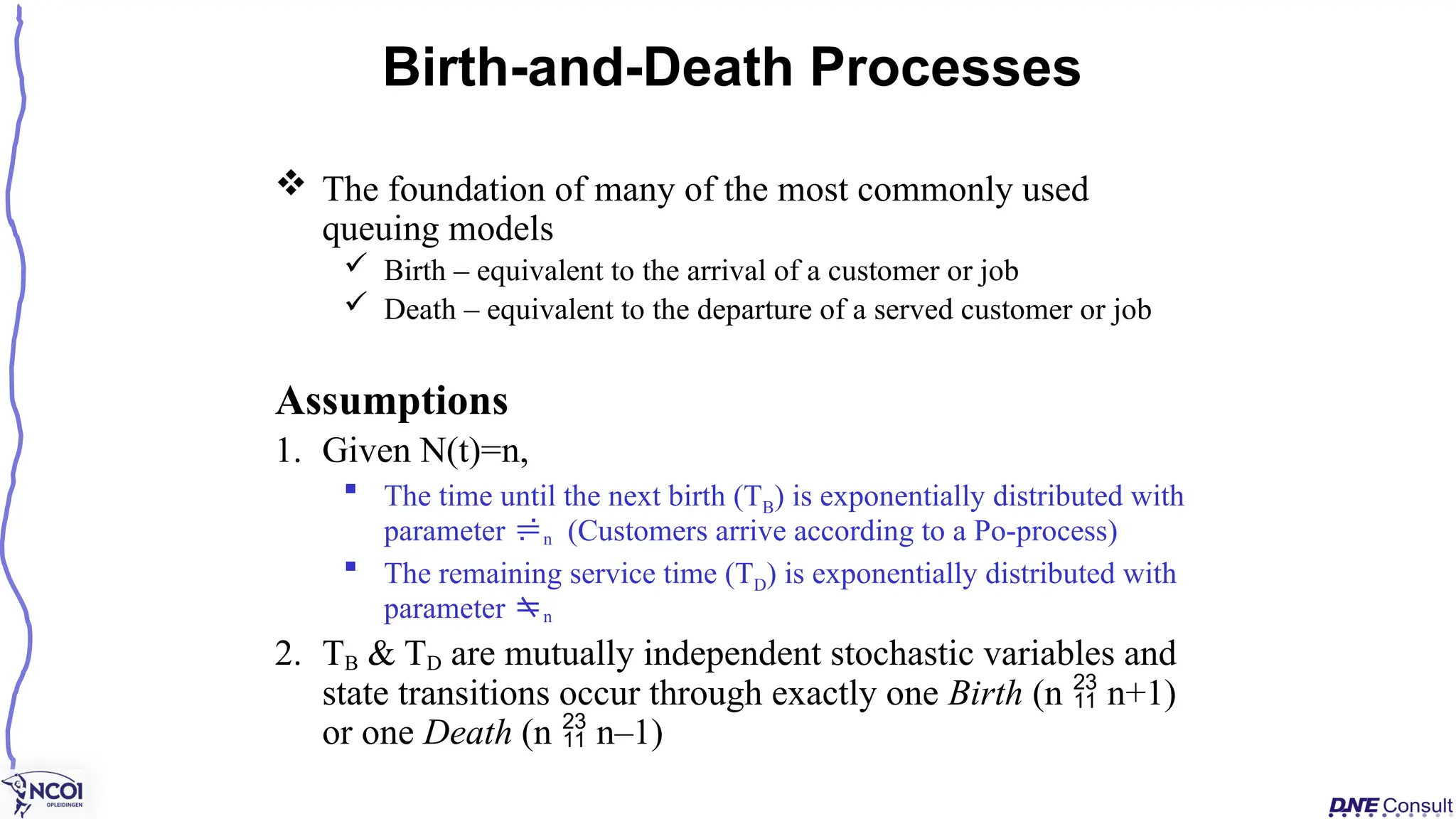
The foundationof many of the most commonly used
queuing models
Birth – equivalent to the arrival of a customer or job
Death – equivalent to the departure of a served customer or job
Assumptions
1. Given N(t)=n,
The time until the next birth (TB) is exponentially distributed with
parameter n (Customers arrive according to a Po-process)
The remaining service time (TD) is exponentially distributed with
parameter n
2. TB & TD are mutually independent stochastic variables and
state transitions occur through exactly one Birth (n n+1)
or one Death (n n–1)
Birth-and-Death Processes
137.
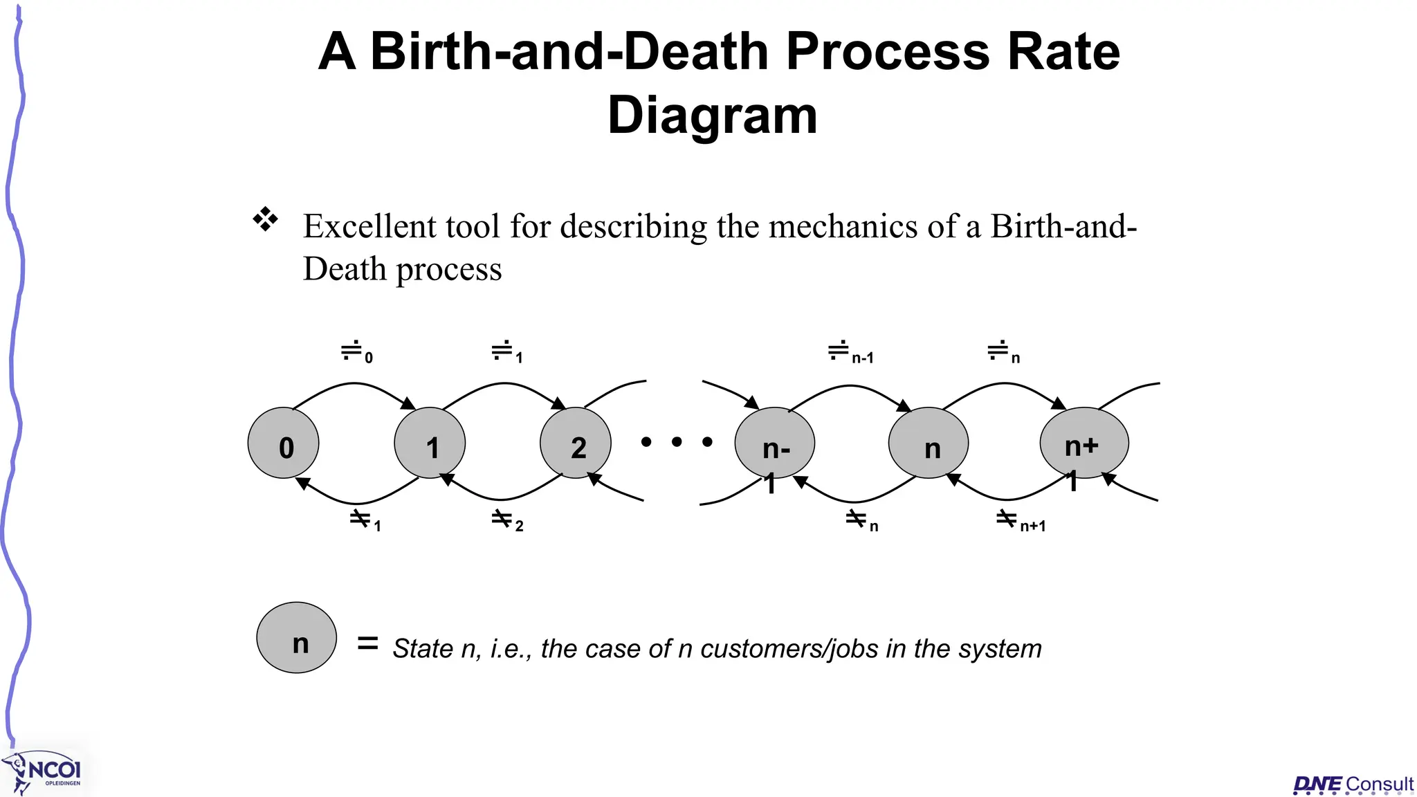
A Birth-and-Death ProcessRate
Diagram
0 1 n-1 n
0 1 2 n-
1
n n+
1
1 2 n n+1
n = State n, i.e., the case of n customers/jobs in the system
Excellent tool for describing the mechanics of a Birth-and-
Death process
138.
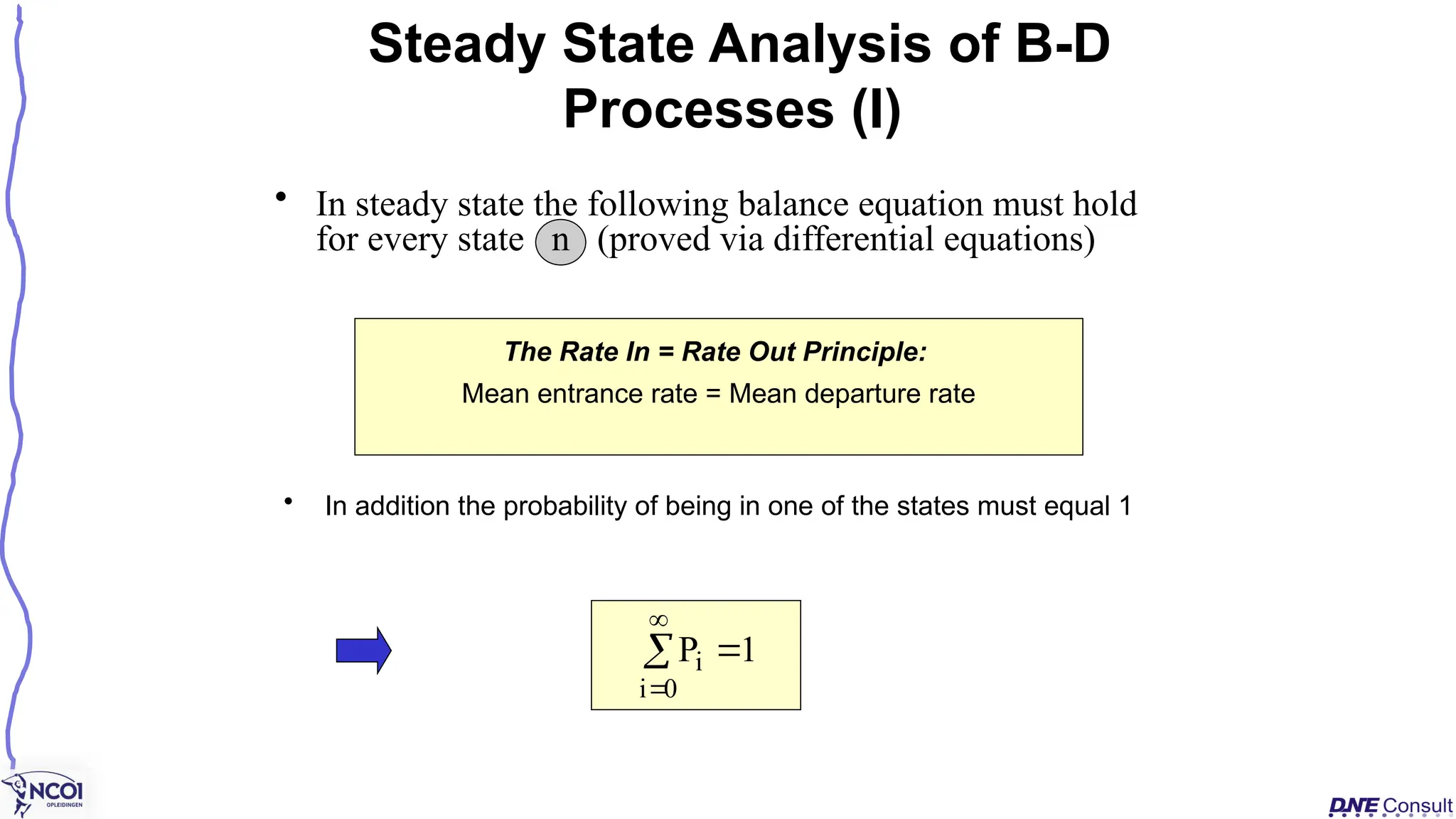
• In steadystate the following balance equation must hold
for every state n (proved via differential equations)
Steady State Analysis of B-D
Processes (I)
The Rate In = Rate Out Principle:
Mean entrance rate = Mean departure rate
0
i
i 1
P
• In addition the probability of being in one of the states must equal 1
139.
0
0
1
1 P
P
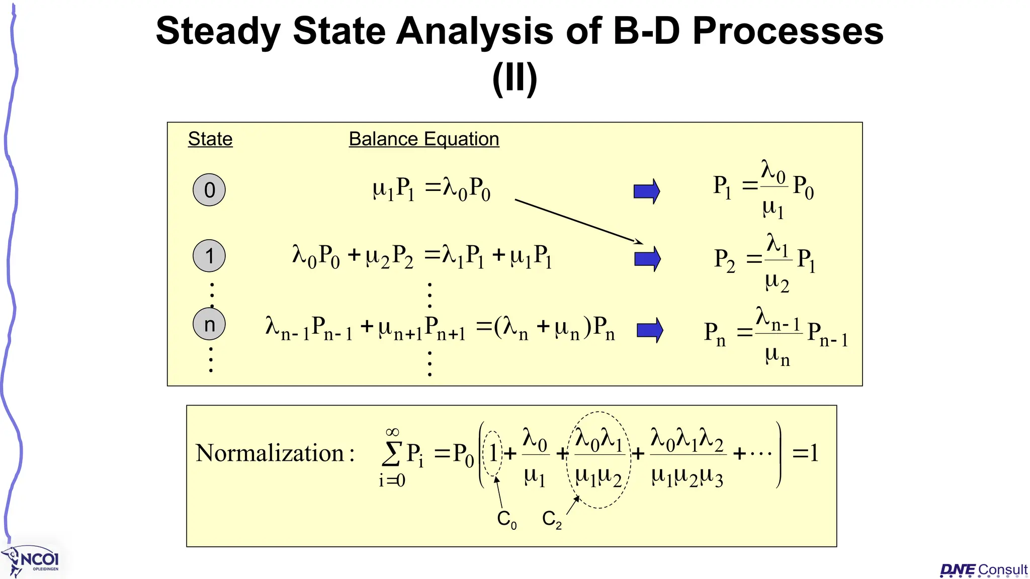
StateBalance Equation
0
1
n
1
1
1
1
2
2
0
0 P
P
P
P
n
n
n
1
n
1
n
1
n
1
n P
)
(
P
P
Steady State Analysis of B-D Processes
(II)
0
1
0
1 P
P
1
2
1
2 P
P
1
n
n
1
n
n P
P
1
1
P
P
:
ion
Normalizat
0
i 3
2
1
2
1
0
2
1
1
0
1
0
0
i
C0 C2
140.
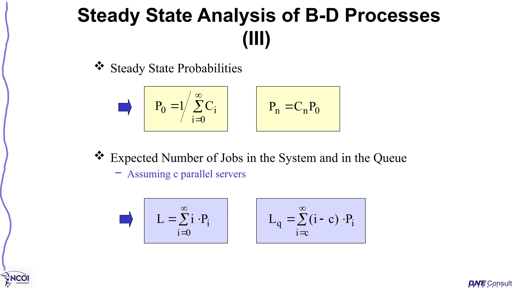
Steady StateProbabilities
Expected Number of Jobs in the System and in the Queue
– Assuming c parallel servers
Steady State Analysis of B-D Processes
(III)
0
i
i
0 C
1
P 0
n
n P
C
P
0
i
i
P
i
L
c
i
i
q P
)
c
i
(
L
141.
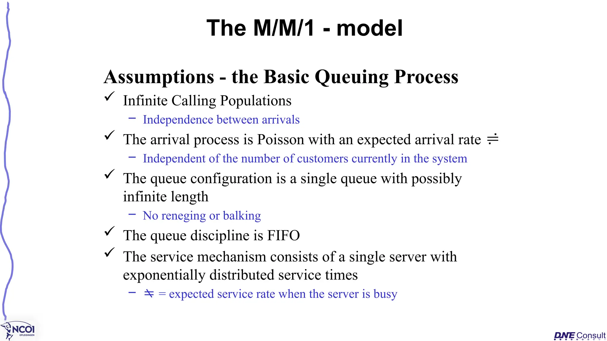
Assumptions - theBasic Queuing Process
Infinite Calling Populations
– Independence between arrivals
The arrival process is Poisson with an expected arrival rate
– Independent of the number of customers currently in the system
The queue configuration is a single queue with possibly
infinite length
– No reneging or balking
The queue discipline is FIFO
The service mechanism consists of a single server with
exponentially distributed service times
– = expected service rate when the server is busy
The M/M/1 - model
142.
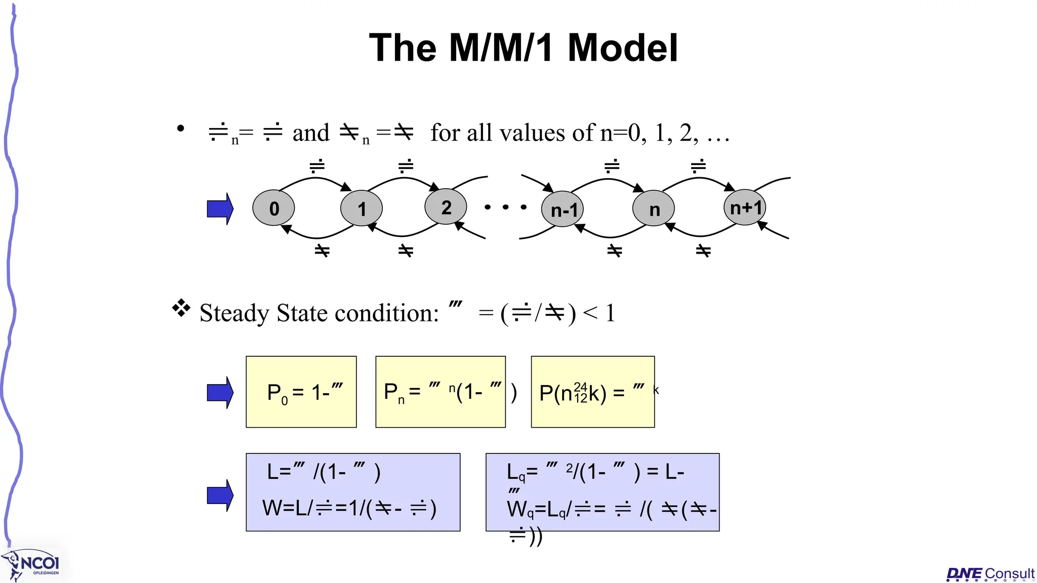
• n= and n = for all values of n=0, 1, 2, …
The M/M/1 Model
0
1 n
n-1
2 n+1
L=/(1- ) Lq= 2
/(1- ) = L-
W=L/=1/(- ) Wq=Lq/= /( (-
))
Steady State condition: = (/) < 1
Pn = n
(1- )
P0 = 1- P(nk) = k
143.
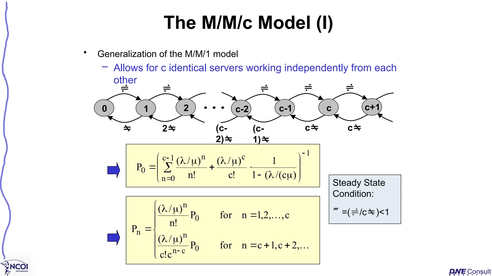
The M/M/c Model(I)
1
c
1
c
0
n
n
0
)
c
/(
(
1
1
!
c
)
/
(
!
n
)
/
(
P
,
2
c
,
1
c
n
for
P
c
!
c
)
/
(
c
,
,
2
,
1
n
for
P
!
n
)
/
(
P
0
c
n
n
0
n
n
0
2 (c-
1)
c
1 c
c-2
2 c+1
c
c-1
(c-
2)
• Generalization of the M/M/1 model
– Allows for c identical servers working independently from each
other
Steady State
Condition:
=(/c)<1
144.
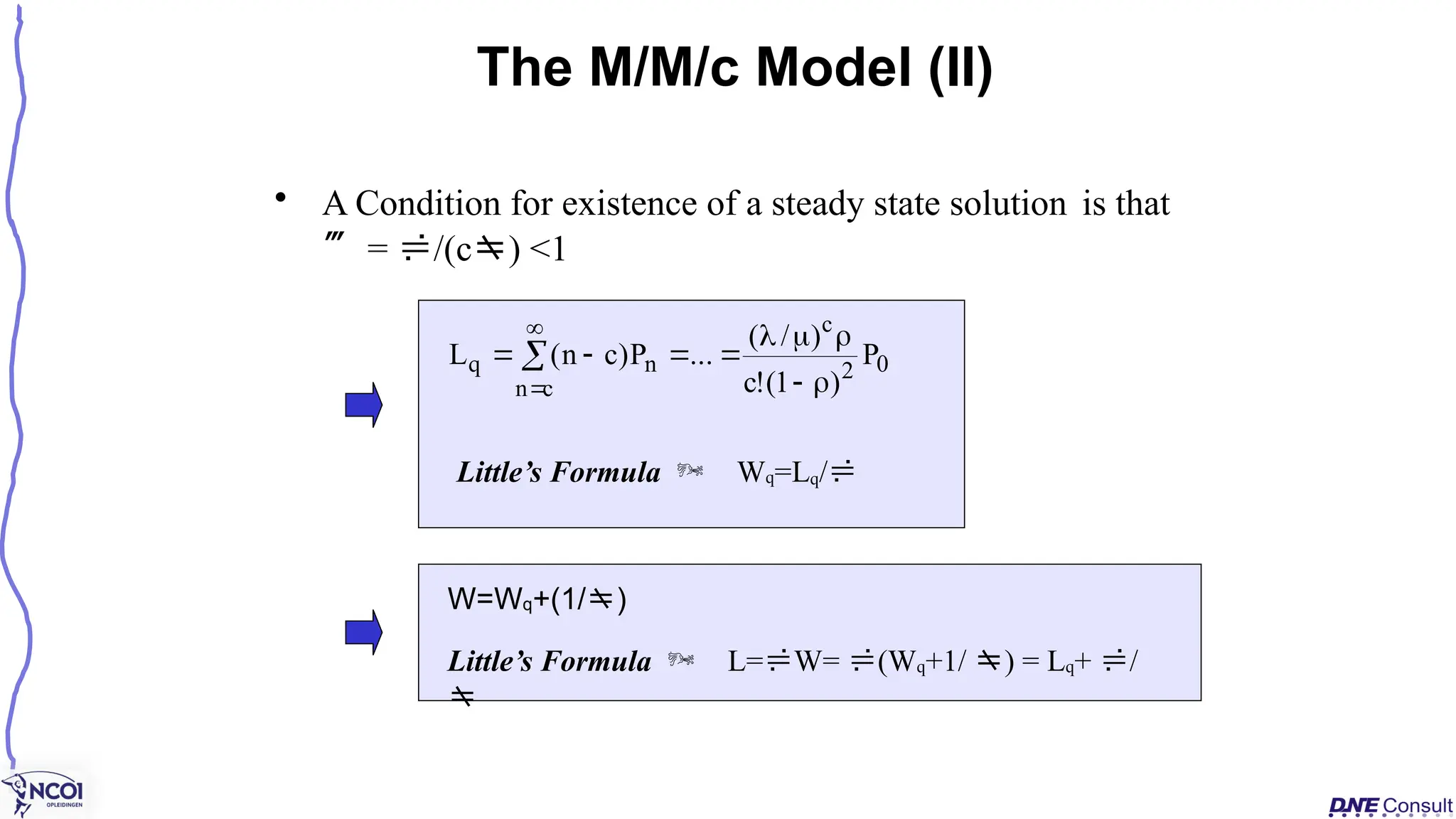
W=Wq+(1/)
Little’s Formula Wq=Lq/
The M/M/c Model (II)
0
2
c
c
n
n
q P
)
1
(
!
c
)
/
(
...
P
)
c
n
(
L
• A Condition for existence of a steady state solution is that
= /(c) <1
Little’s Formula L=W= (Wq+1/ ) = Lq+ /
145.
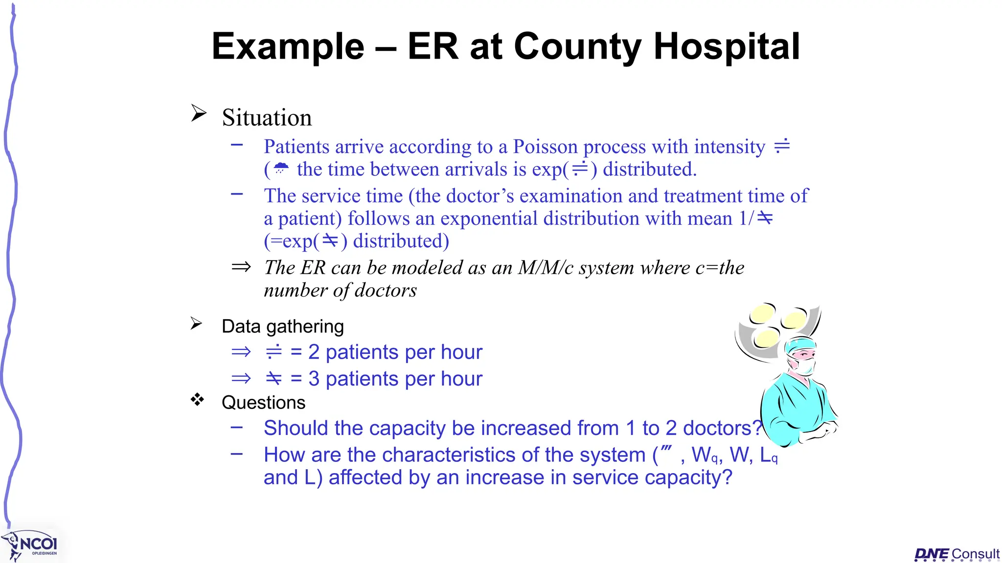
Situation
– Patientsarrive according to a Poisson process with intensity
( the time between arrivals is exp() distributed.
– The service time (the doctor’s examination and treatment time of
a patient) follows an exponential distribution with mean 1/
(=exp() distributed)
Þ The ER can be modeled as an M/M/c system where c=the
number of doctors
Example – ER at County Hospital
Data gathering
Þ = 2 patients per hour
Þ = 3 patients per hour
Questions
– Should the capacity be increased from 1 to 2 doctors?
– How are the characteristics of the system (, Wq, W, Lq
and L) affected by an increase in service capacity?
146.
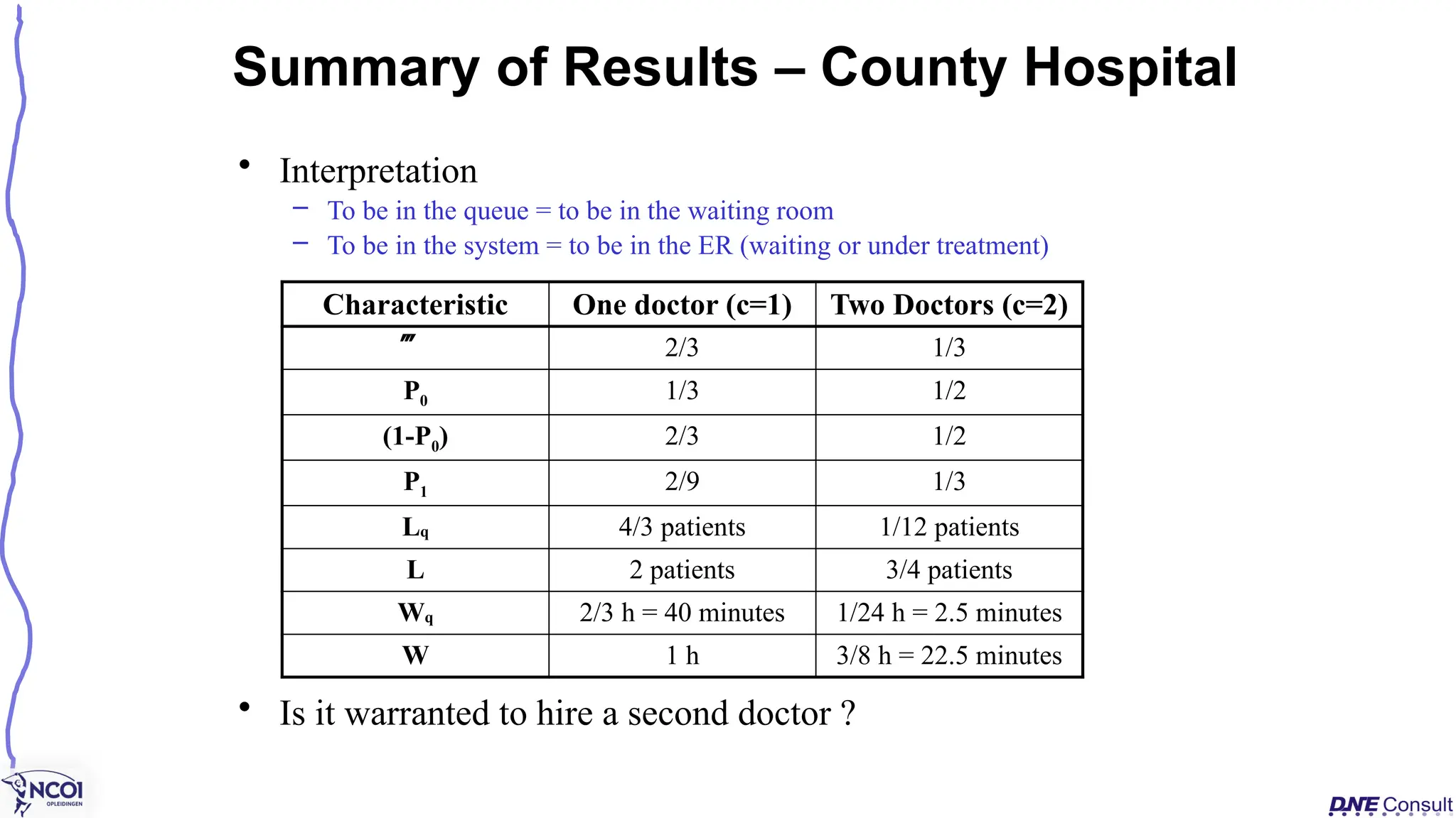
• Interpretation
– Tobe in the queue = to be in the waiting room
– To be in the system = to be in the ER (waiting or under treatment)
• Is it warranted to hire a second doctor ?
Summary of Results – County Hospital
Characteristic One doctor (c=1) Two Doctors (c=2)
2/3 1/3
P0 1/3 1/2
(1-P0) 2/3 1/2
P1 2/9 1/3
Lq 4/3 patients 1/12 patients
L 2 patients 3/4 patients
Wq 2/3 h = 40 minutes 1/24 h = 2.5 minutes
W 1 h 3/8 h = 22.5 minutes
147.
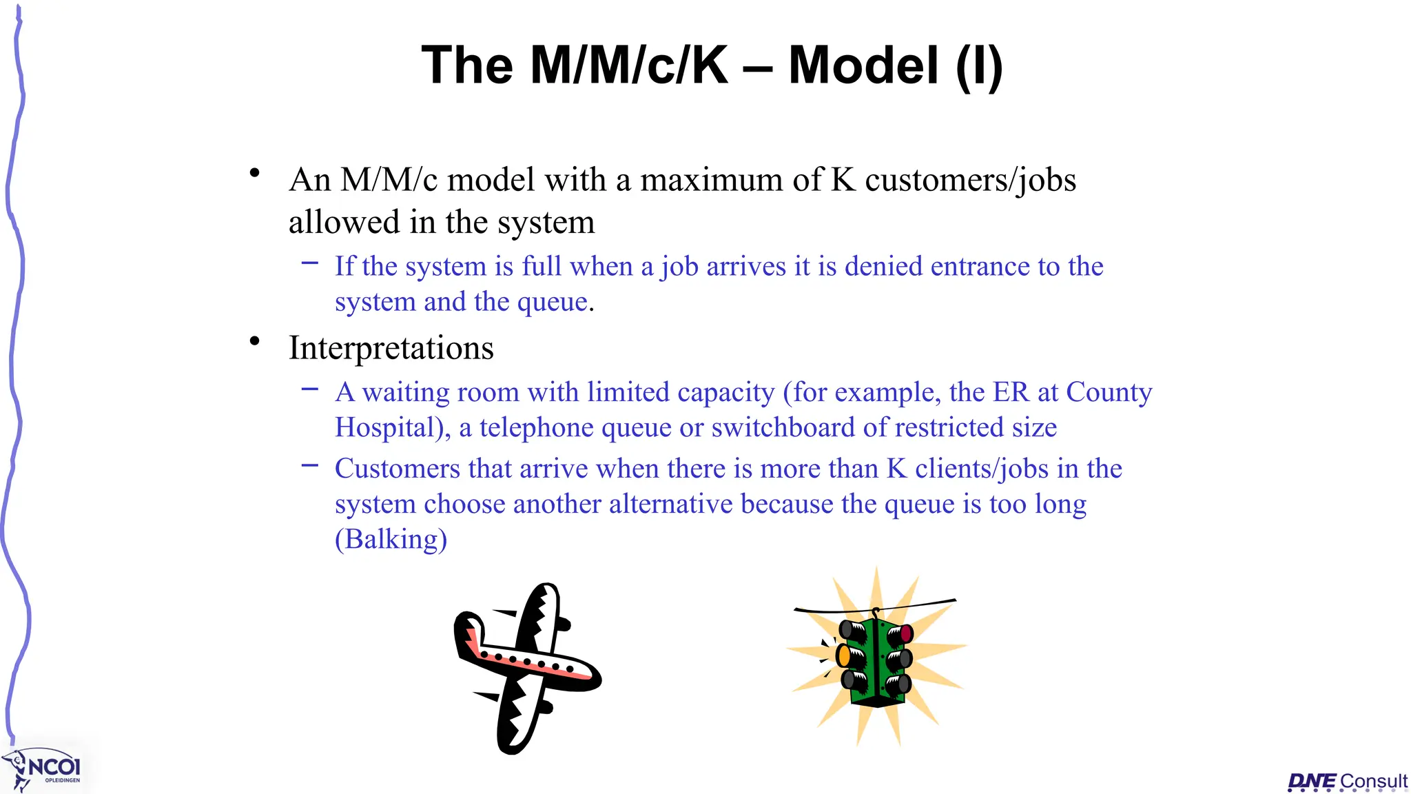
• An M/M/cmodel with a maximum of K customers/jobs
allowed in the system
– If the system is full when a job arrives it is denied entrance to the
system and the queue.
• Interpretations
– A waiting room with limited capacity (for example, the ER at County
Hospital), a telephone queue or switchboard of restricted size
– Customers that arrive when there is more than K clients/jobs in the
system choose another alternative because the queue is too long
(Balking)
The M/M/c/K – Model (I)
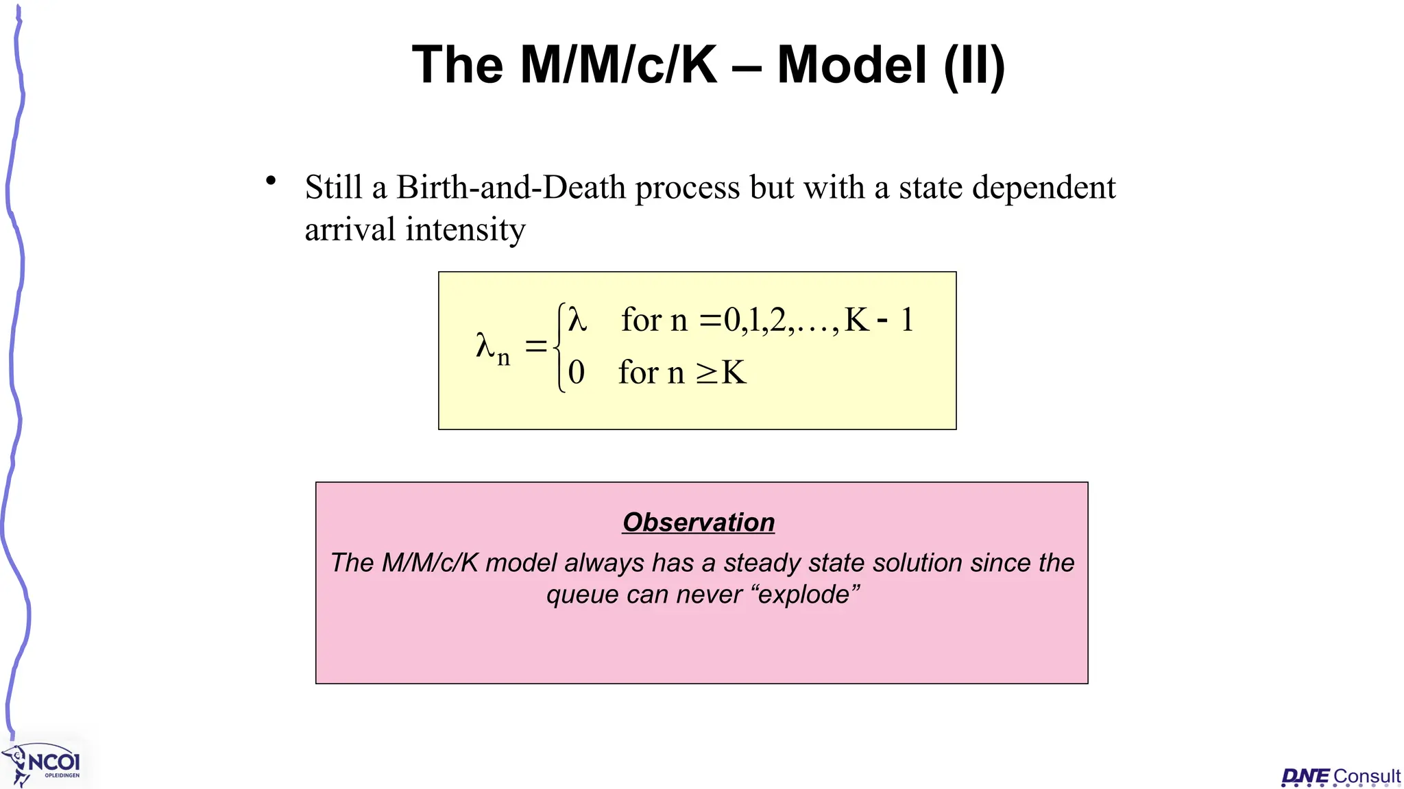
148.
• Still aBirth-and-Death process but with a state dependent
arrival intensity
The M/M/c/K – Model (II)
K
n
for
0
1
K
,
,
2
,
1
,
0
n
for
n
Observation
The M/M/c/K model always has a steady state solution since the
queue can never “explode”
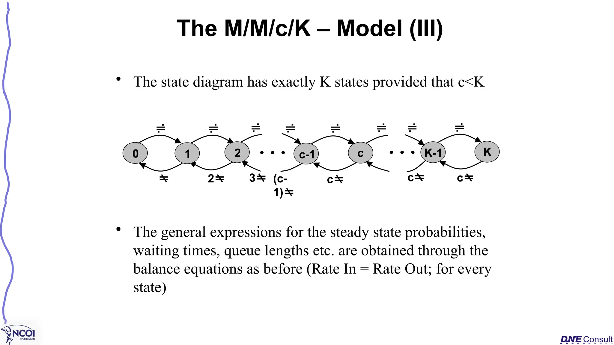
149.
• The statediagram has exactly K states provided that c<K
• The general expressions for the steady state probabilities,
waiting times, queue lengths etc. are obtained through the
balance equations as before (Rate In = Rate Out; for every
state)
The M/M/c/K – Model (III)
0
2 (c-
1)
c
1 K-1
c-1
2 K
c
c
c
3
150.
• For = (/) 1
Results for the M/M/1/K – Model
1
K
0
1
1
P
n
1
K
0
n
n
1
1
P
P
1
K
1
K
1
)
1
K
(
1
L
)
P
1
(
L
L 0
q
/
L
W
/
L
W q
q
0
n
n
nP
Where
151.
• An M/M/cmodel with limited calling population, i.e., N
clients
• A common application: Machine maintenance
– c service technicians is responsible for keeping N service stations
(machines) running, that is, to repair them as soon as they break
– Customer/job arrivals = machine breakdowns
– Note, the maximum number of clients in the system = N
• Assume that (N-n) machines are operating and the time until
breakdown for each machine i, Ti, is exponentially distributed
(Tiexp()). If U = the time until the next breakdown
Þ U = Min{T1, T2, …, TN-n} Uexp((N-n))).
The M/M/c//N – Model (I)
152.
• The StateDiagram (c service technicians and N machines)
– = Arrival intensity per operating machine
– = The service intensity for a service technician
• General expressions for this queuing model can be obtained from the
balance equations as before
The M/M/c//N – Model (II)
0
N
(N-1) (N-(c-
1))
2 (c-
1)
c
1 N-1
c-1
2 N
c
c
3
153.
• For situationswhere different customers have different
priorities
– For example, ER operations, VIP customers at nightclubs…
• Assuming a situation with N priority classes (where class 1 has
the highest priority) there are two fundamental priority
principles to consider.
1. Non-Preemptive priorities
A customer being served cannot be ejected back into the queue to
leave place for a customer with higher priority
2. Preemptive priorities
A customer of lower priority that is being served will be thrown
back into the queue to leave room for a higher priority customer
• Assuming that all customers experience independent exp()
service times and arrive according to Poisson processes both
models can be analyzed as special case M/M/c models
Priority-Discipline Queuing Models
154.
• Design ofqueuing systems usually involve some kind of
capacity decision
– The number of service stations
– The number of servers per station
– The service time for individual servers
ÞThe corresponding decision variables are , c and
• Examples:
– The number of doctors in a hospital,
– The number of exits and cashiers in a supermarket,
– The choice of machine type at a new investment decision,
– The localization of toilets in a new building, etc…
Queuing Modeling and System Design
(I)
155.
• Two fundamentalquestions when designing (queuing)
systems
– Which service level should we aim for?
– How much capacity should we acquire?
• The cost of increased capacity must be balanced against
the cost reduction due to shorter waiting time
Þ Specify a waiting cost or a shortage cost accruing when
customers have to wait for service or…
Þ … Specify an acceptable service level and minimize the capacity
under this condition
• The shortage or waiting cost rate is situation dependent and
often difficult to quantify
– Should reflect the monetary impact a delay has on the
organization where the queuing system resides
Queuing Modeling and System Design
(II)
156.
1. External customersarrive to the system
• Profit organizations
Þ The shortage cost is primarily related to lost revenues –
“Bad Will”
• Non-profit organizations
Þ The shortage cost is related to a societal cost
2. Internal customers arrive to the system
Þ The shortage cost is related to productivity loss and associated
profit loss
• Usually it is easier to estimate the shortage costs in
situation 2. than in situation 1.
Different Shortage Cost Situations
157.
• Given aspecified shortage or waiting cost function the analysis
is straightforward
• Define
– WC = Expected Waiting Cost (shortage cost) per time unit
– SC = Expected Service Cost (capacity cost) per time unit
– TC = Expected Total system cost per time unit
• The objective is to minimize the total expected system cost
Analyzing Design-Cost Tradeoffs
Min TC = WC + SC
Process capacity
Cost
WC
SC
TC
158.
• Expected WaitingCosts as a function of the number of
customers in the system
– Cw = Waiting cost per customer and time unit
– CwN = Waiting cost per time unit when N customers in the system
Analyzing Linear Waiting Costs
L
C
nP
C
WC w
0
n
n
w
• Expected Waiting Costs as a function of the number of customers in the
queue
q
wL
C
WC
159.
SC = c*CS()
The expected service costs per time unit, SC, depend on the
number of servers and their speed
• Definitions
– c = Number of servers
– = Average server intensity (average time to serve one
customer)
– CS() = Expected cost per server and time unit as a function
of
Analyzing Service Costs
160.
Determining andc
• Both the number of servers and their speed can be varied
– Usually only a few alternatives are available
• Definitions
– A = The set of available - options
A Decision Model for System Design
WC
)
(
C
c
TC
Min s
,...
1
,
0
c
,
A
From a structural point of view, a few fast servers are usually better than
several slow ones with the same maximum capacity
• Optimization
– Enumerate all interesting combinations of and c, compute TC
and choose the cheapest alternative
161.
• A universityis about to lease a super computer
• There are two alternatives available
– The M computer which is more expensive to lease but also faster
– The C computer which is cheaper but slower
• Processing times and times between job arrivals
are exponential M/M/1 model
– = 20 jobs per day
– M = 30 jobs per day
– C = 25 jobs per day
• The leasing and waiting costs:
– Leasing price: CM = $500 per day, CC = $350 per day
– The waiting cost per job and time unit job is estimated to $50 per job
and day
• Question:
– Which computer should the university choose in order to minimize the
expected costs?
Example – “Computer Procurement”
162.
Dado Cukor
Lecturer ofInnovation & Strategic Management
Member of board of examiners (Master & Bachelor)
NCOI Business School
d.cukor@gmail.com
www.linkedin.com/in/cukor
+31 6 5160 36 88
Bedankt
Slides are available: e-connect
Think Free & don’t forget a Fun
Voorbereiding:
• Voorbereidingsopdracht: Enkelvoudig procesmodel in Excel (Single step Model)
• Meervoudig Procesmodel in Excel (Multiple step Model)
Editor's Notes
#94 After this slide it is suitable with a larger example of Cycle Time Analysis, for example, Problems 9 & 10, Chapter 4 in Laguna.
#101 After this slide it is suitable with a larger example of Capacity analysis, for example, Problem 11, Chapter 4 in Laguna.

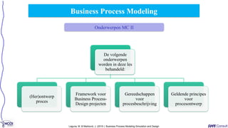
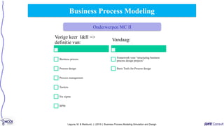
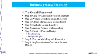
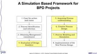

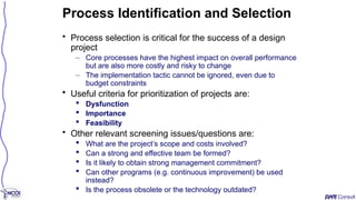


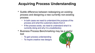
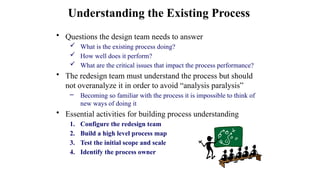


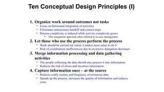
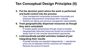
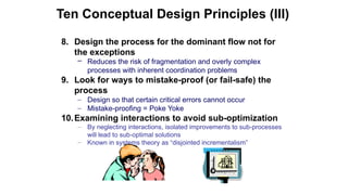


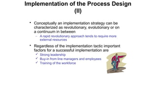


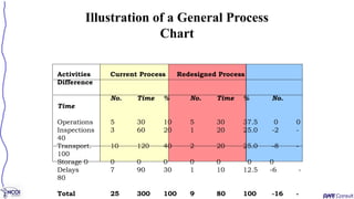

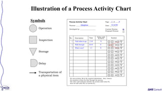


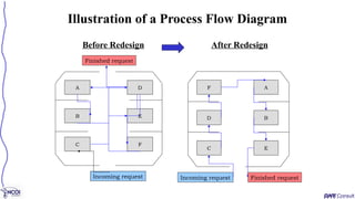
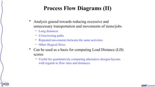
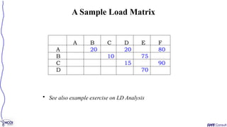

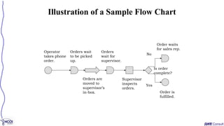
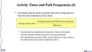

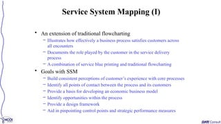

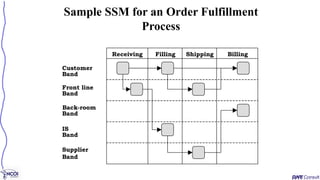

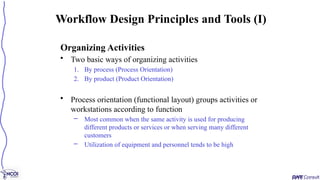

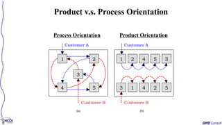
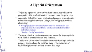
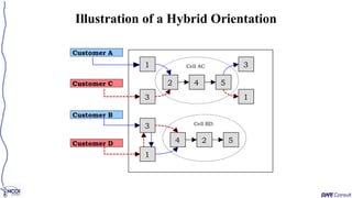

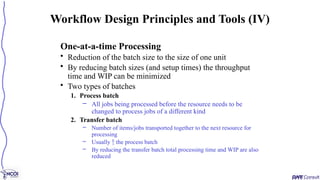
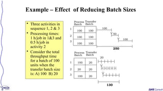

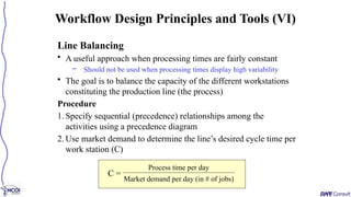
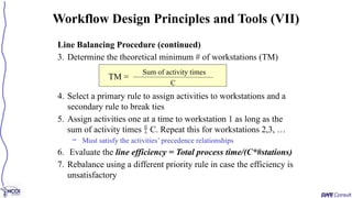

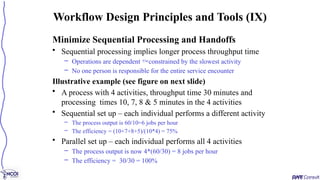

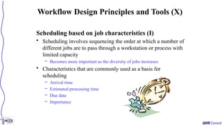

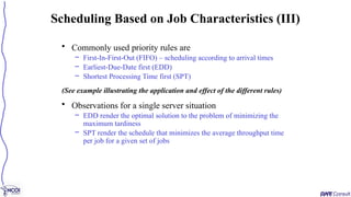
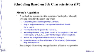


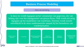
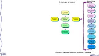

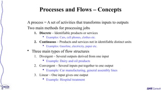
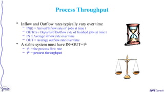
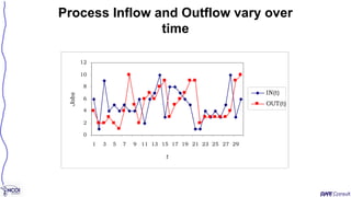

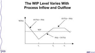
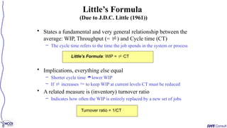
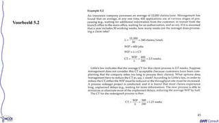
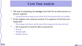
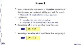

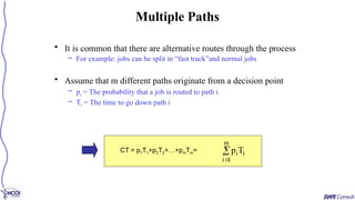
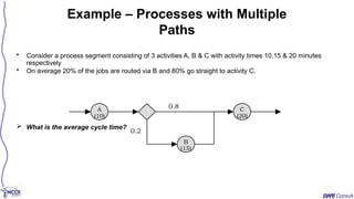
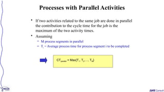
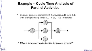

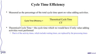
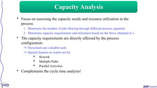

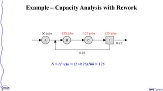
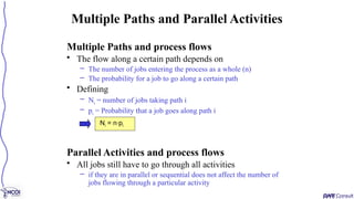
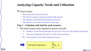
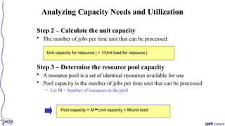
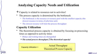
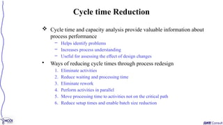
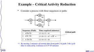
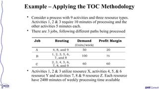


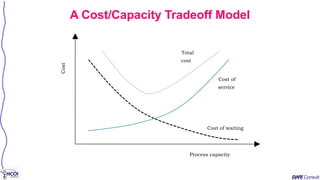
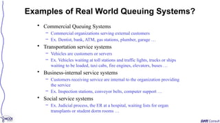
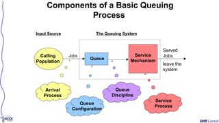

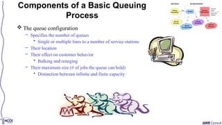


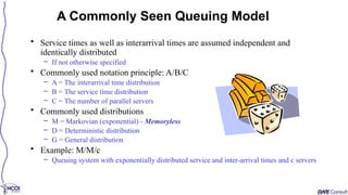
![The most commonly used queuing models are based on the
assumption of exponentially distributed service times and
interarrival times.
Definition: A stochastic (or random) variable Texp( ),
i.e., is exponentially distributed with parameter , if its
frequency function is:
The Exponential Distribution and
Queuing
0
t
when
0
0
t
when
e
)
t
(
f
t
T
t
T e
1
)
t
(
F
The Cumulative Distribution Function is:
The mean = E[T] = 1/
The Variance = Var[T] = 1/ 2
Stochastisch = De aanwezigheid
van een toevalsvariabele.
Een stochastisch proces houdt in dat
het systeem een element van toeval
kent (bijvoorbeeld merkenwissel
wordt vaak als
een stochastisch proces gezien).
T = random variabele representing
either interarrival times or services
times in a queuing proces.](https://image.slidesharecdn.com/mcbpm3-250413093009-970d90f4/85/Business-Process-Modeling-Theory-and-practice-119-320.jpg)
![The Exponential Distribution
Time between arrivals
Mean=
E[T]=1/
Probability
density
t
fT(t)
](https://image.slidesharecdn.com/mcbpm3-250413093009-970d90f4/85/Business-Process-Modeling-Theory-and-practice-120-320.jpg)
![ Relationship to the Poisson distribution and the Poisson Process
Let X(t) be the number of events occurring in the interval
[0,t]. If the time between consecutive events is T and
Texp()
X(t)Po(t) {X(t), t0} constitutes a Poisson Process
Properties of the Exp-distribution (IV)
...
,
1
,
0
n
for
!
n
e
)
t
(
)
n
)
t
(
X
(
P
nt
n
](https://image.slidesharecdn.com/mcbpm3-250413093009-970d90f4/85/Business-Process-Modeling-Theory-and-practice-121-320.jpg)
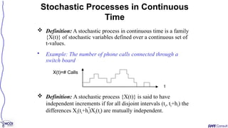
![ The standard assumption in many queuing models is that the
arrival process is Poisson
Two equivalent definitions of the Poisson Process
1. The times between arrivals are independent, identically
distributed and exponential
2. X(t) is a Poisson process with arrival rate iff.
a) X(t) have independent increments
b) For a small time interval h it holds that
P(exactly 1 event occurs in the interval [t, t+h]) = h + o(h)
P(more than 1 event occurs in the interval [t, t+h]) = o(h)
The Poisson Process](https://image.slidesharecdn.com/mcbpm3-250413093009-970d90f4/85/Business-Process-Modeling-Theory-and-practice-123-320.jpg)

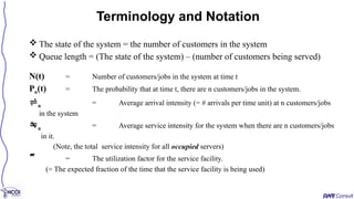


![Transient and Steady State Conditions
• Illustration of transient and steady-state conditions
– N(t) = number of customers in the system at time t,
– E[N(t)] = represents the expected number of customers in the system.
Transient condition
0
5
10
15
20
25
30
0 5 10 15 20 25 30 35 40 45 50
time, t
Number
of
jobs
in
the
system,
N(t)
Steady State condition
E[N(t)]
N(t)](https://image.slidesharecdn.com/mcbpm3-250413093009-970d90f4/85/Business-Process-Modeling-Theory-and-practice-128-320.jpg)


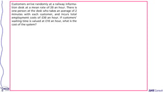
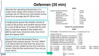
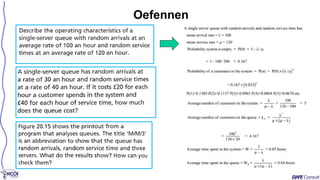

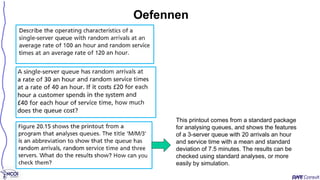
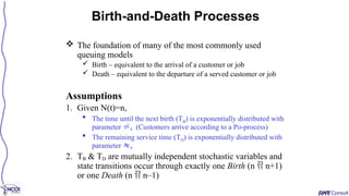


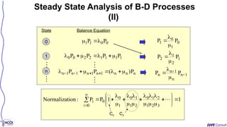
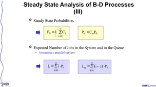

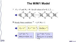
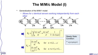
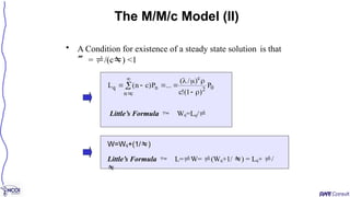
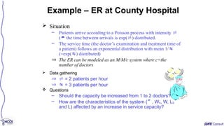
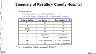


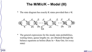
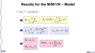
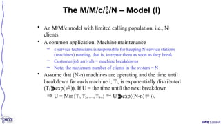
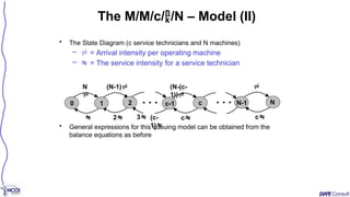
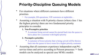


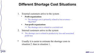

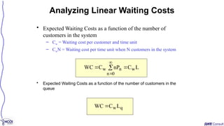
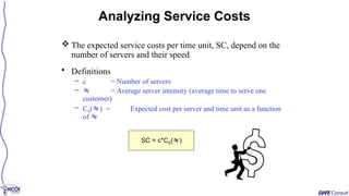


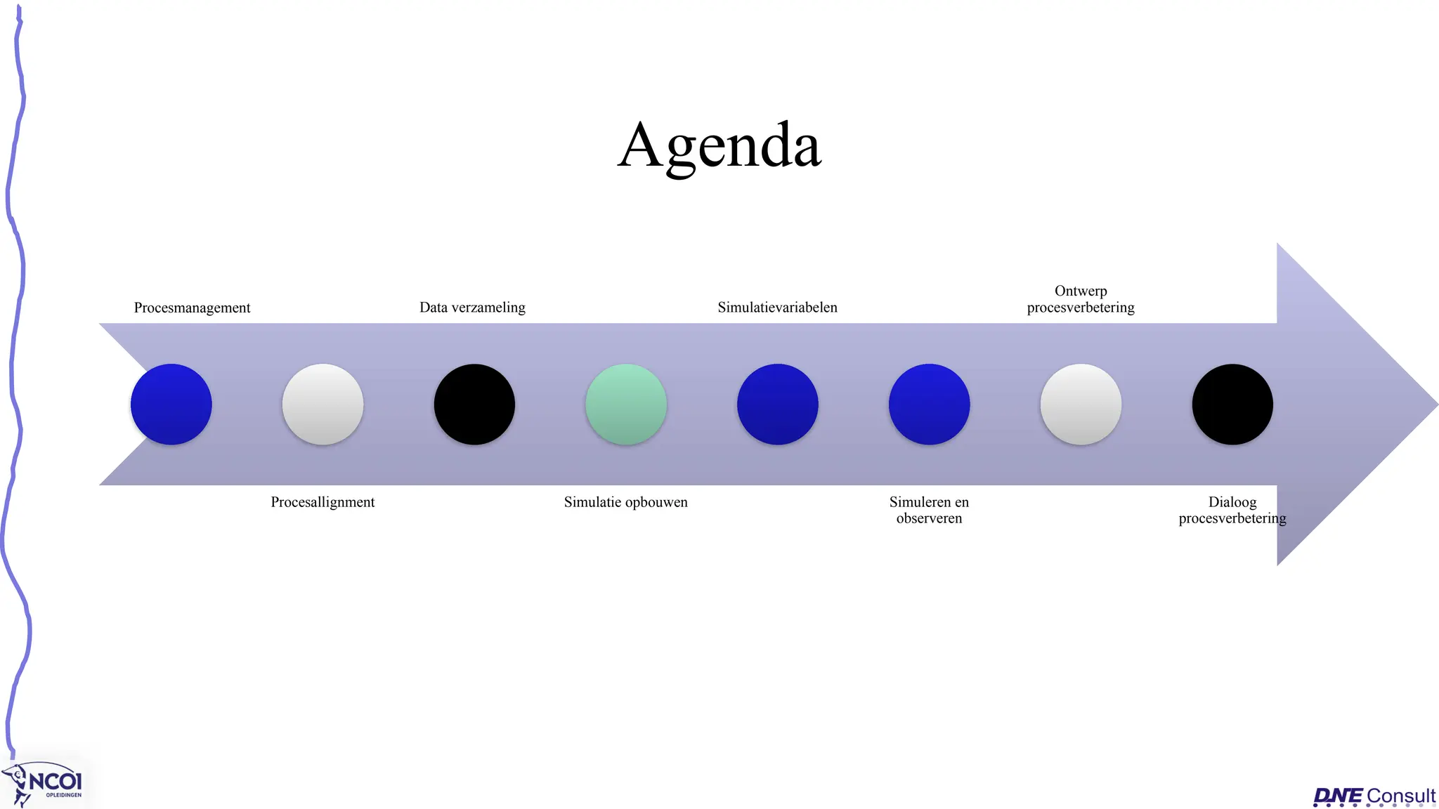
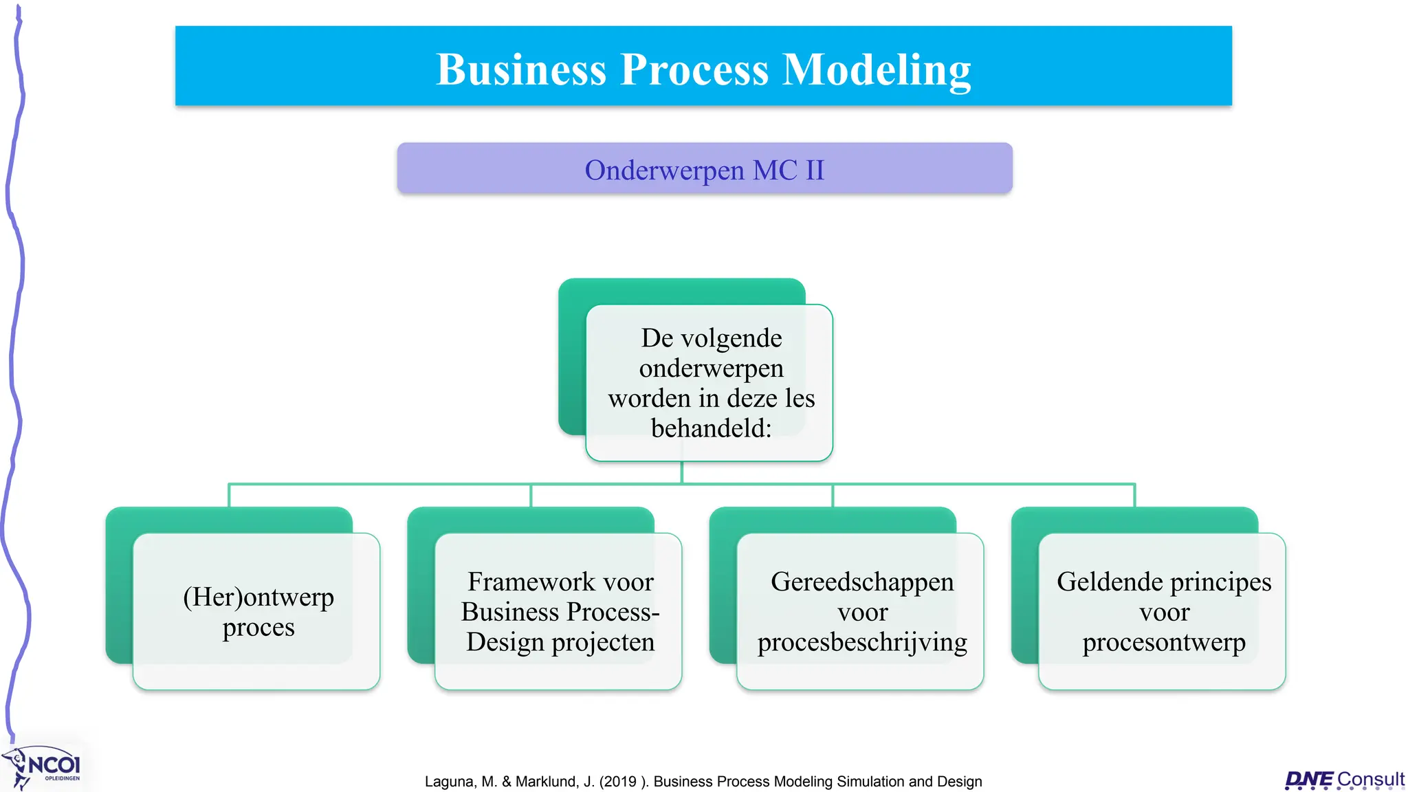
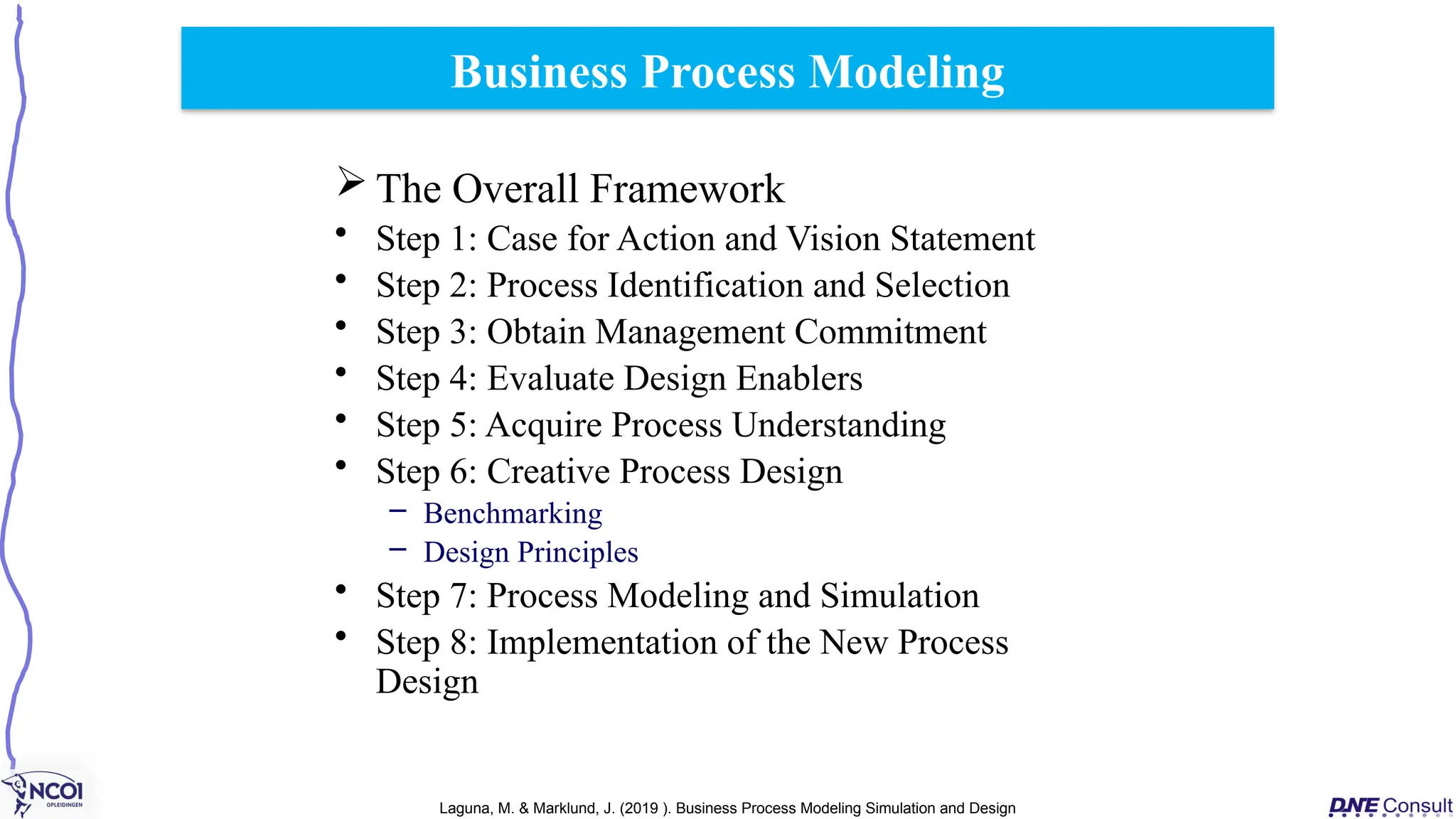
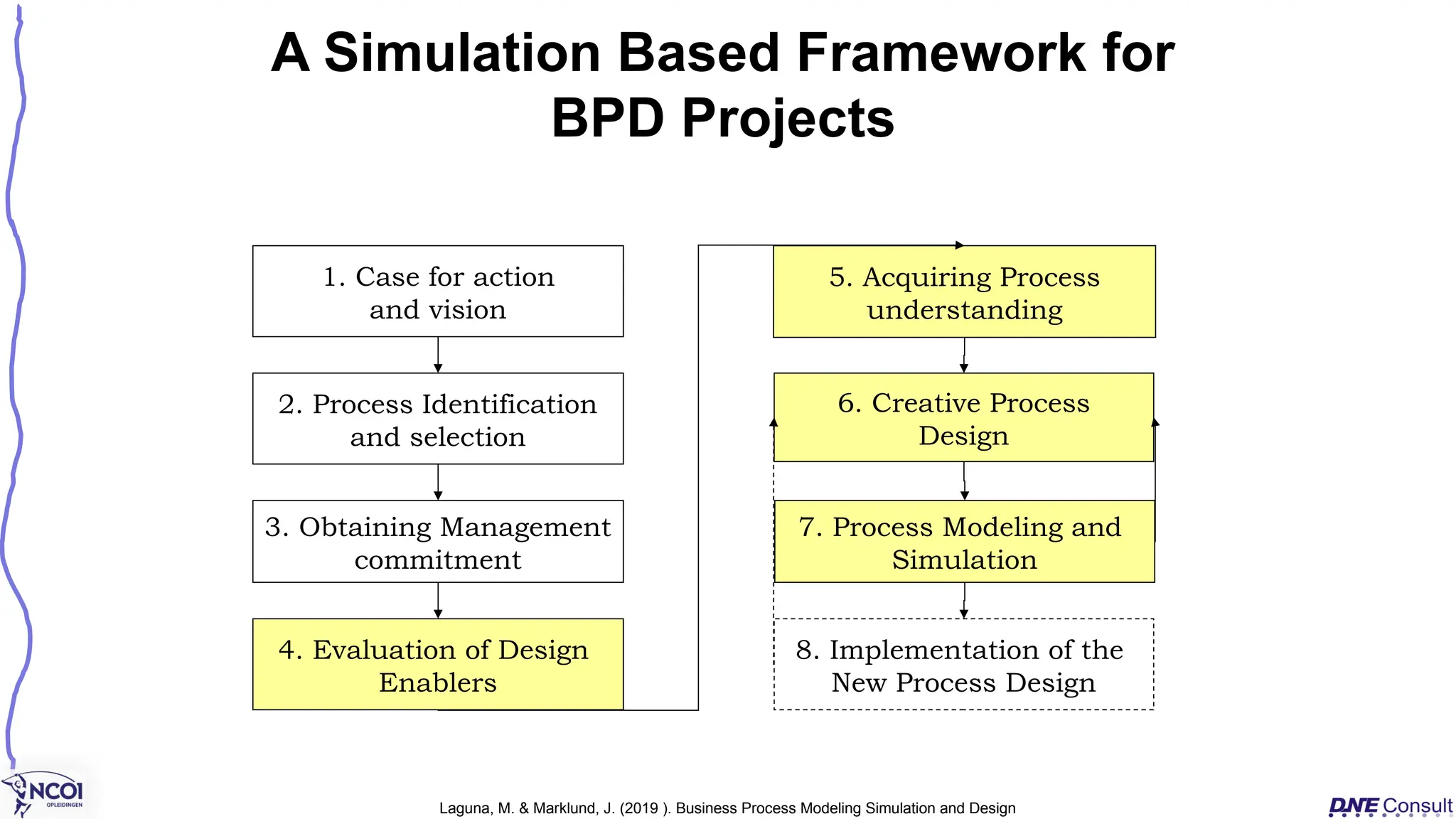
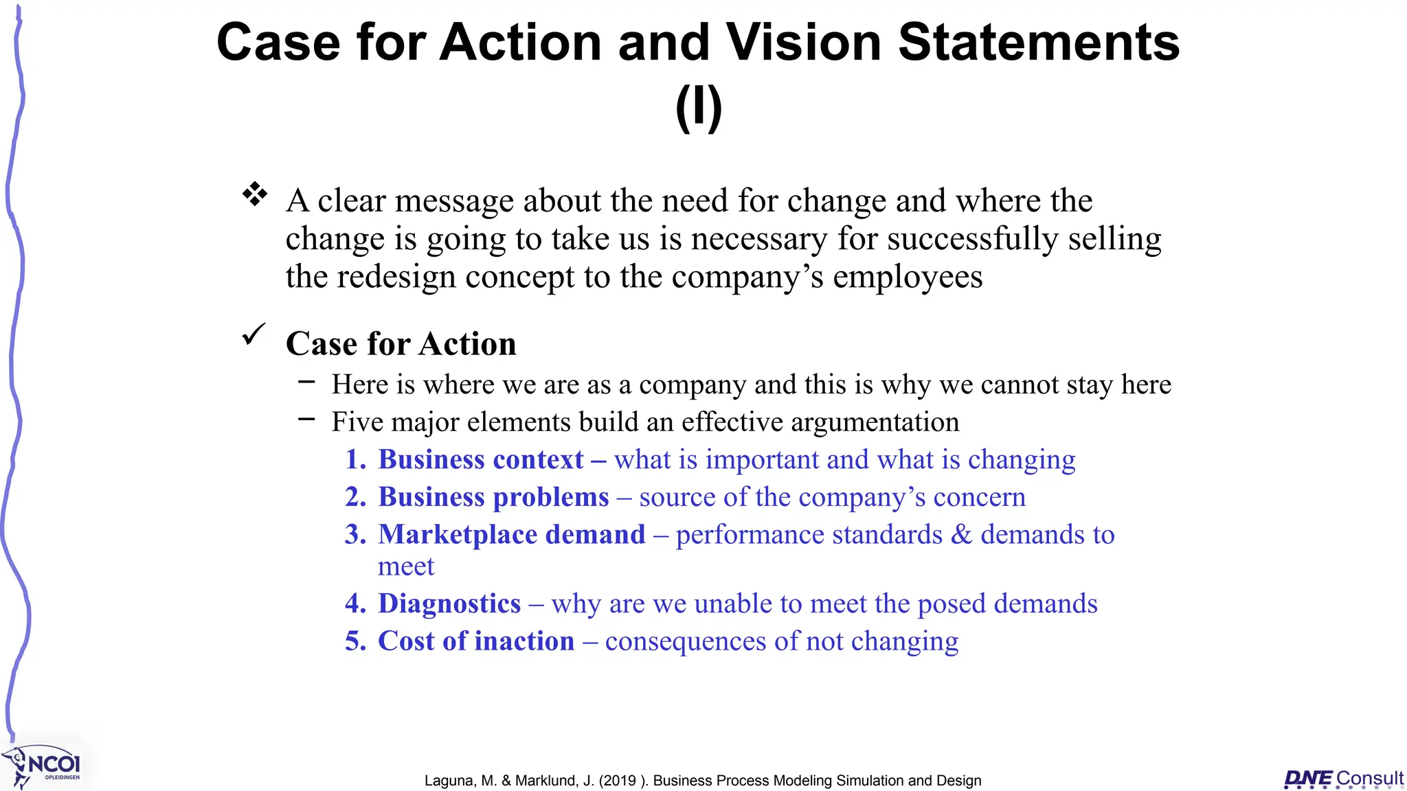
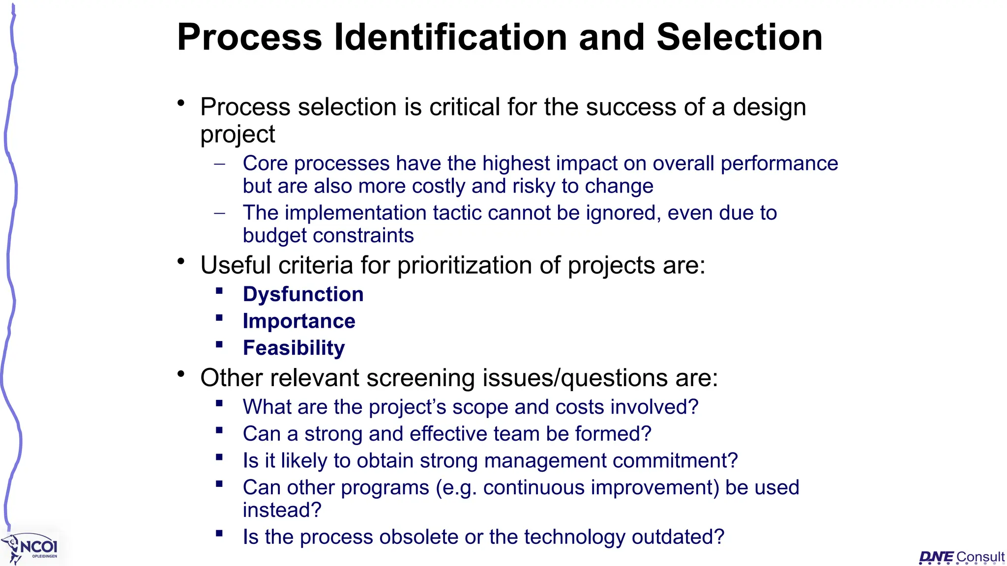

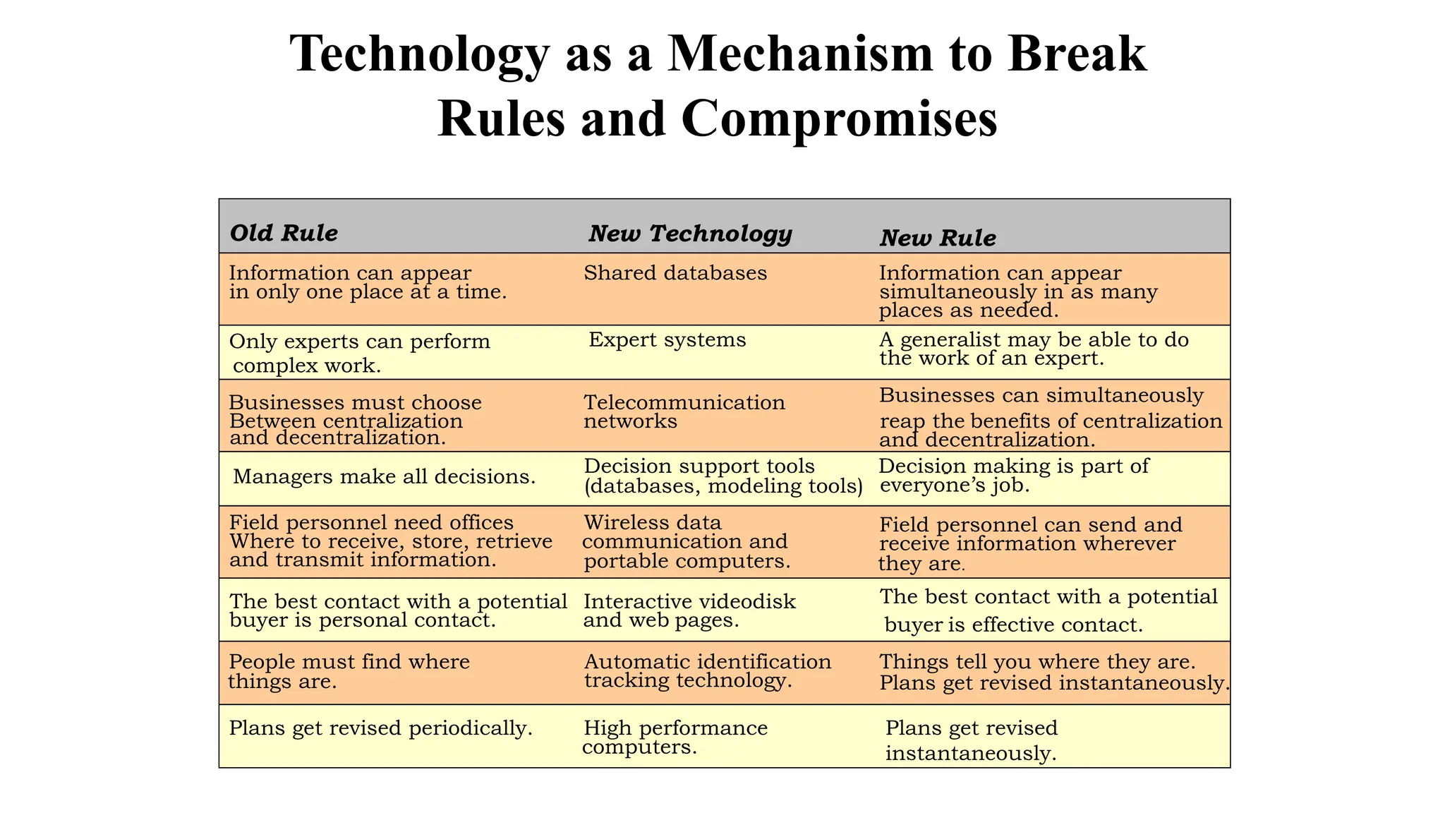
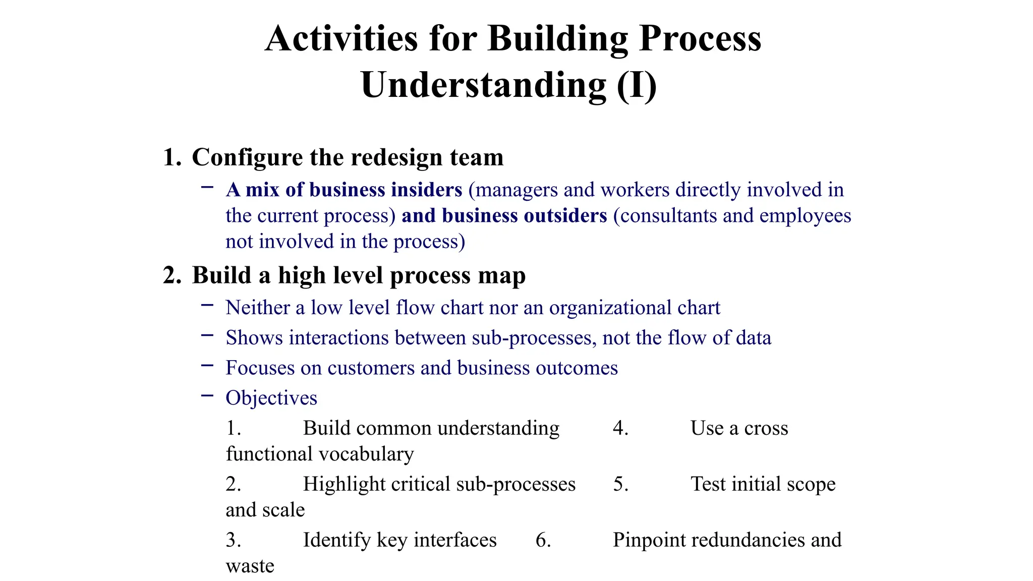

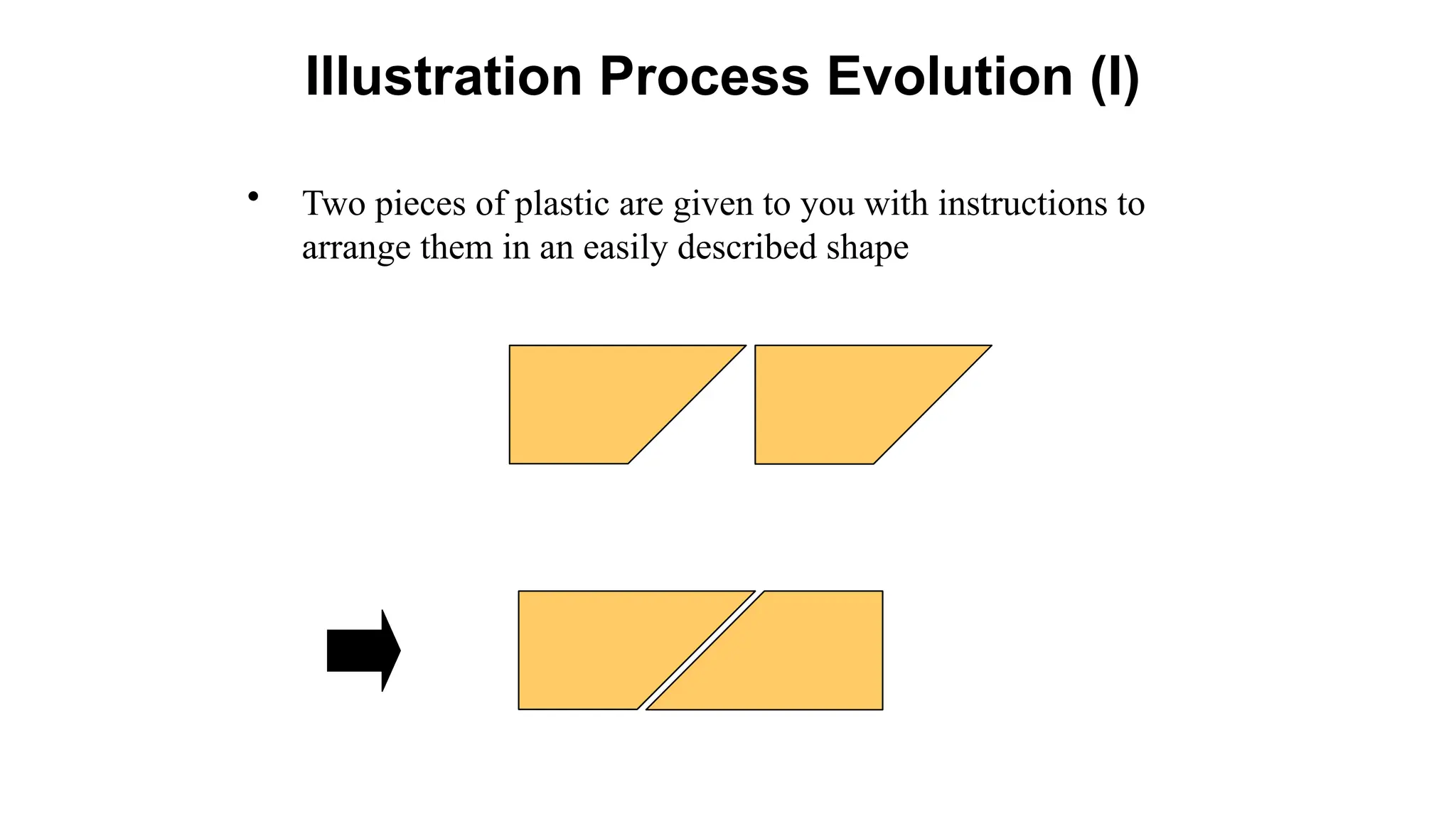
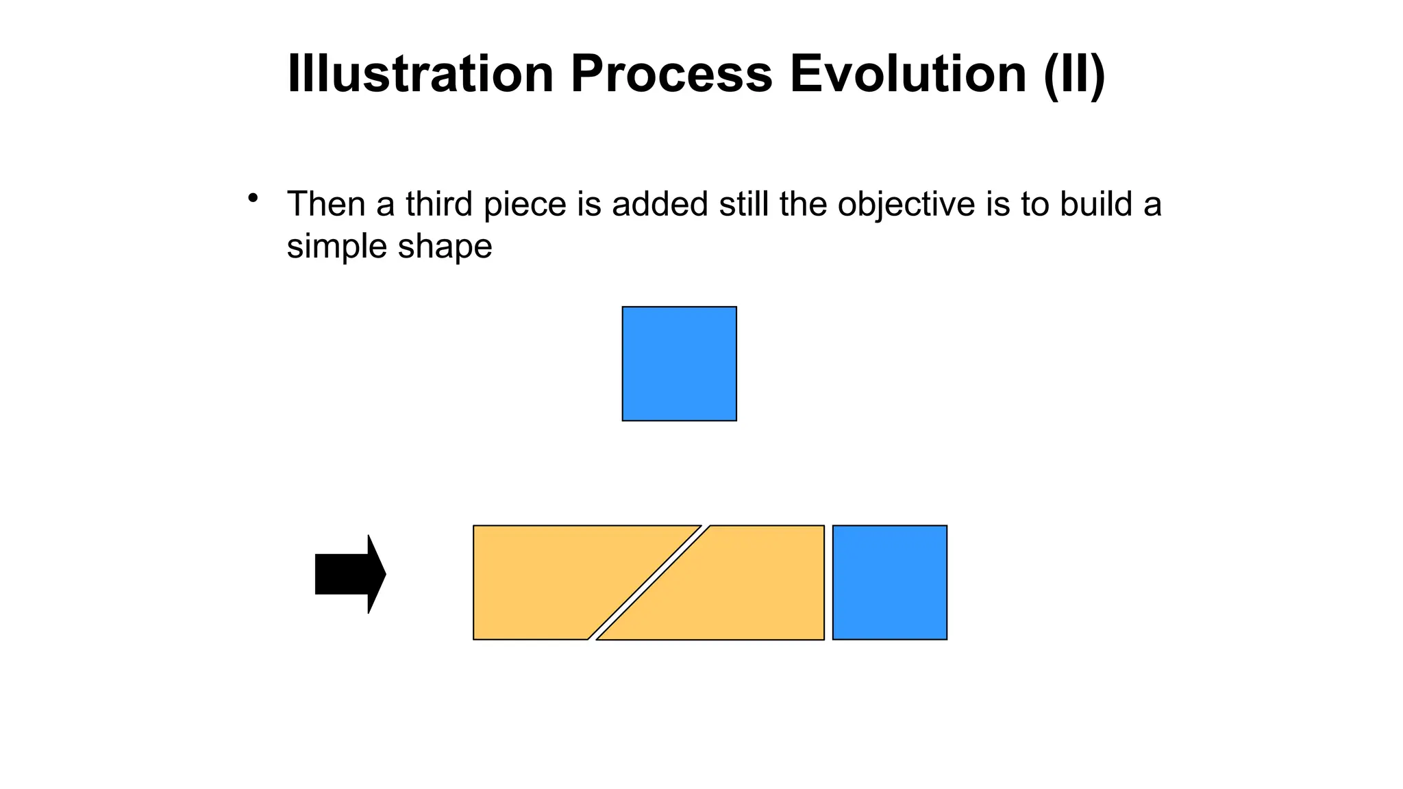
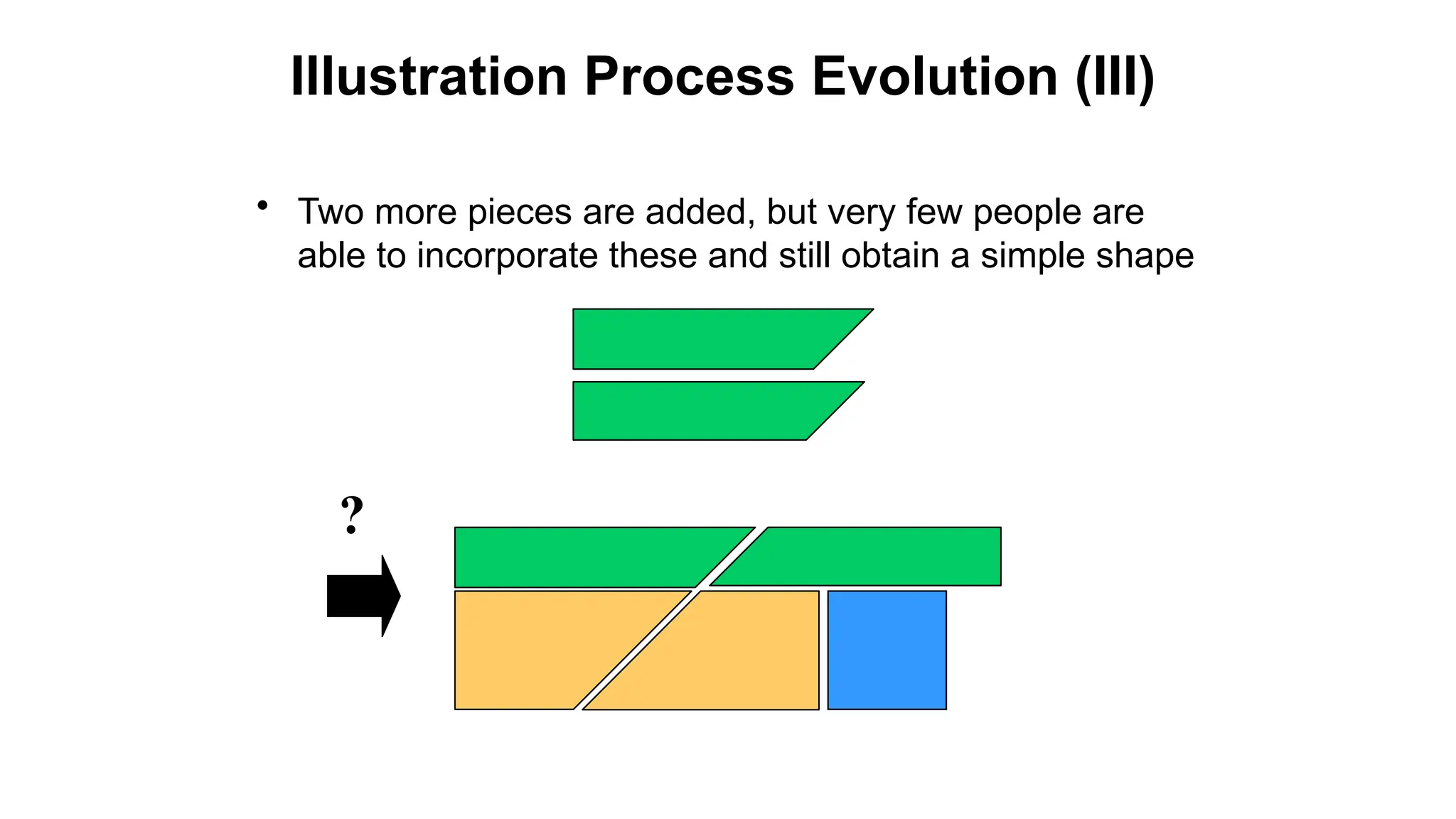
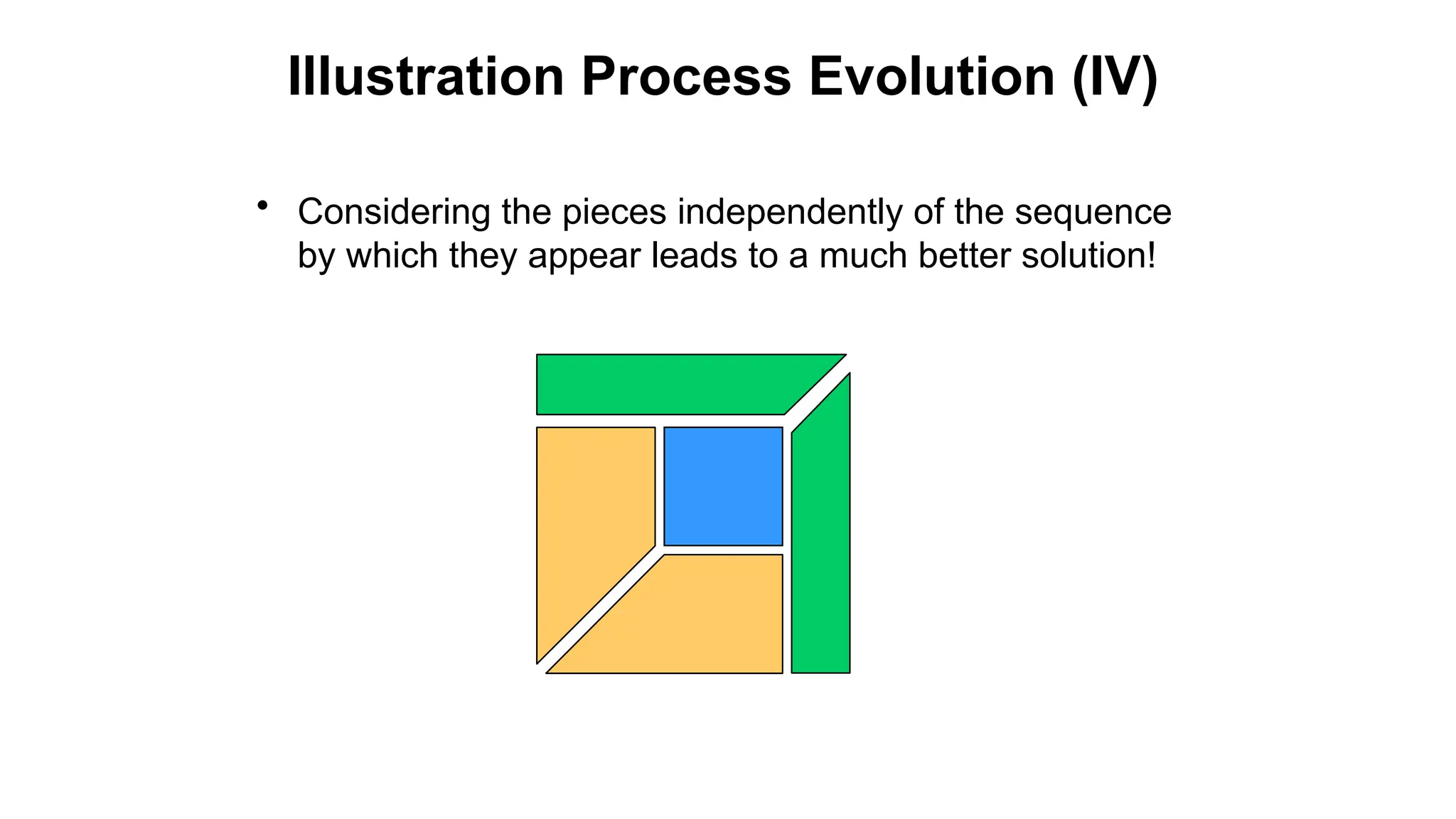
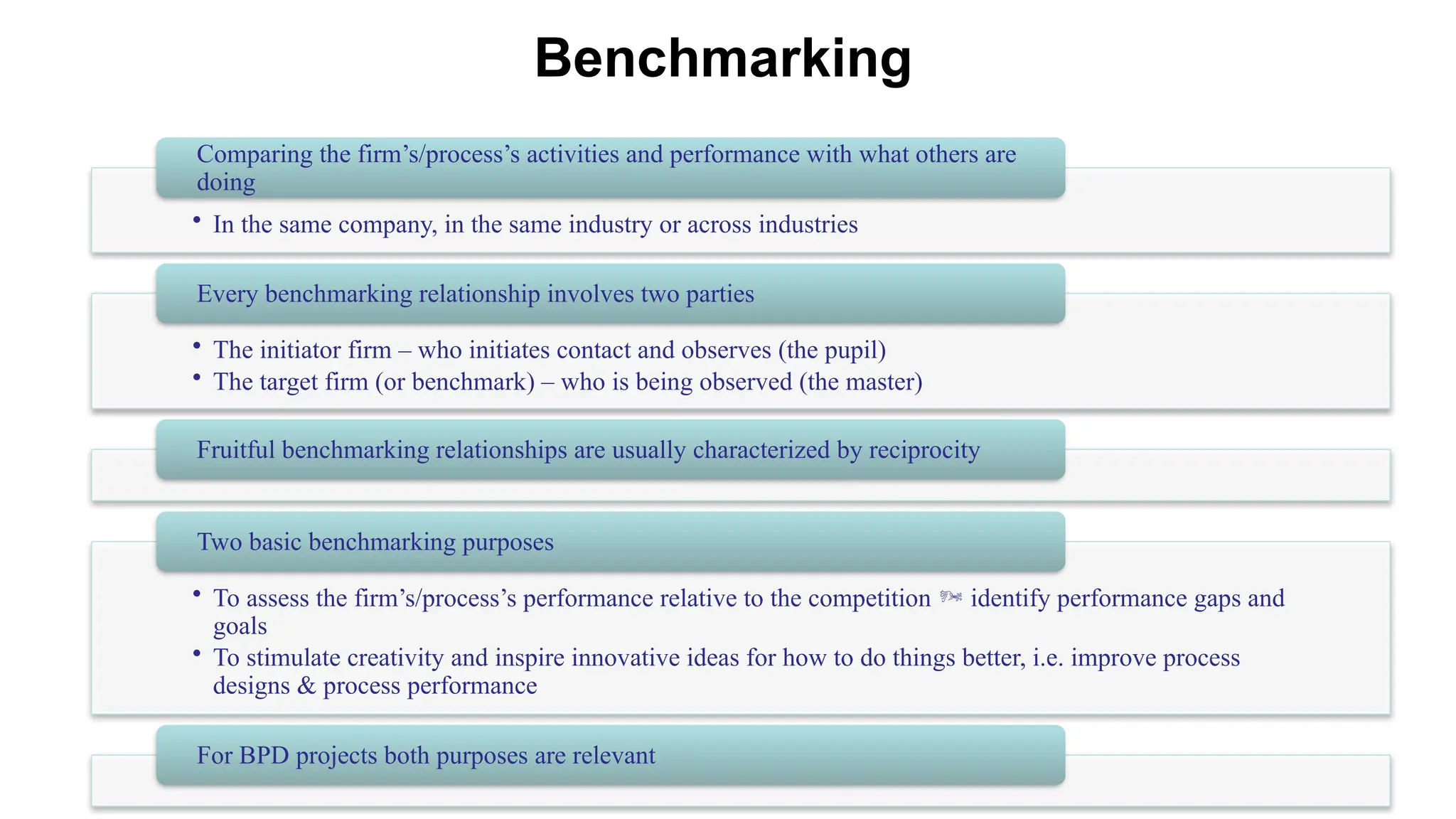
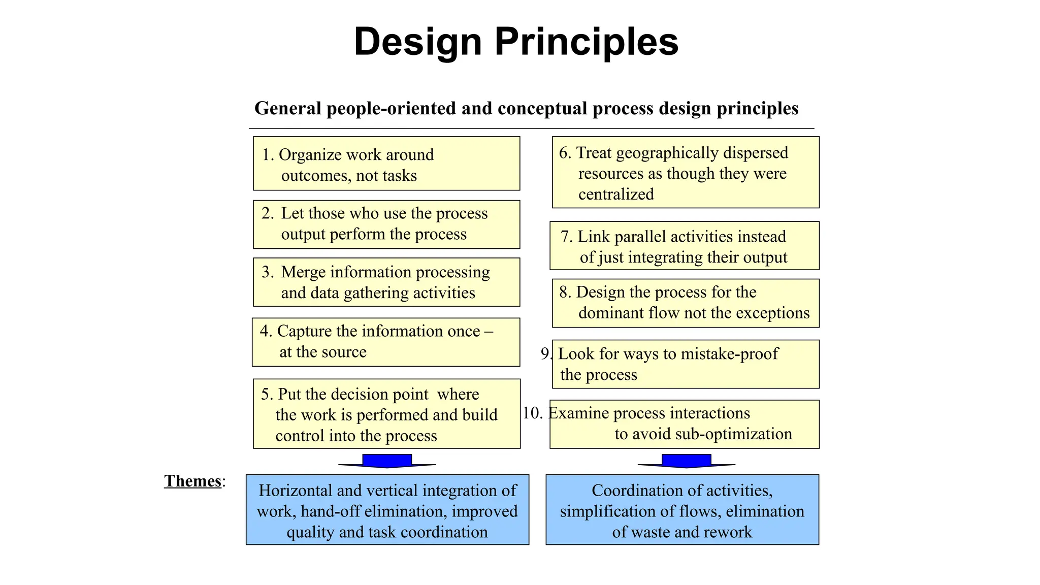


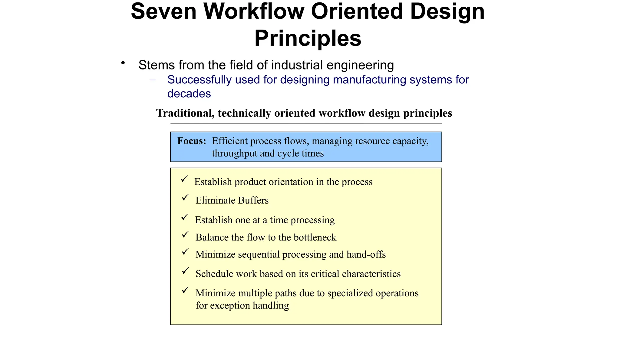
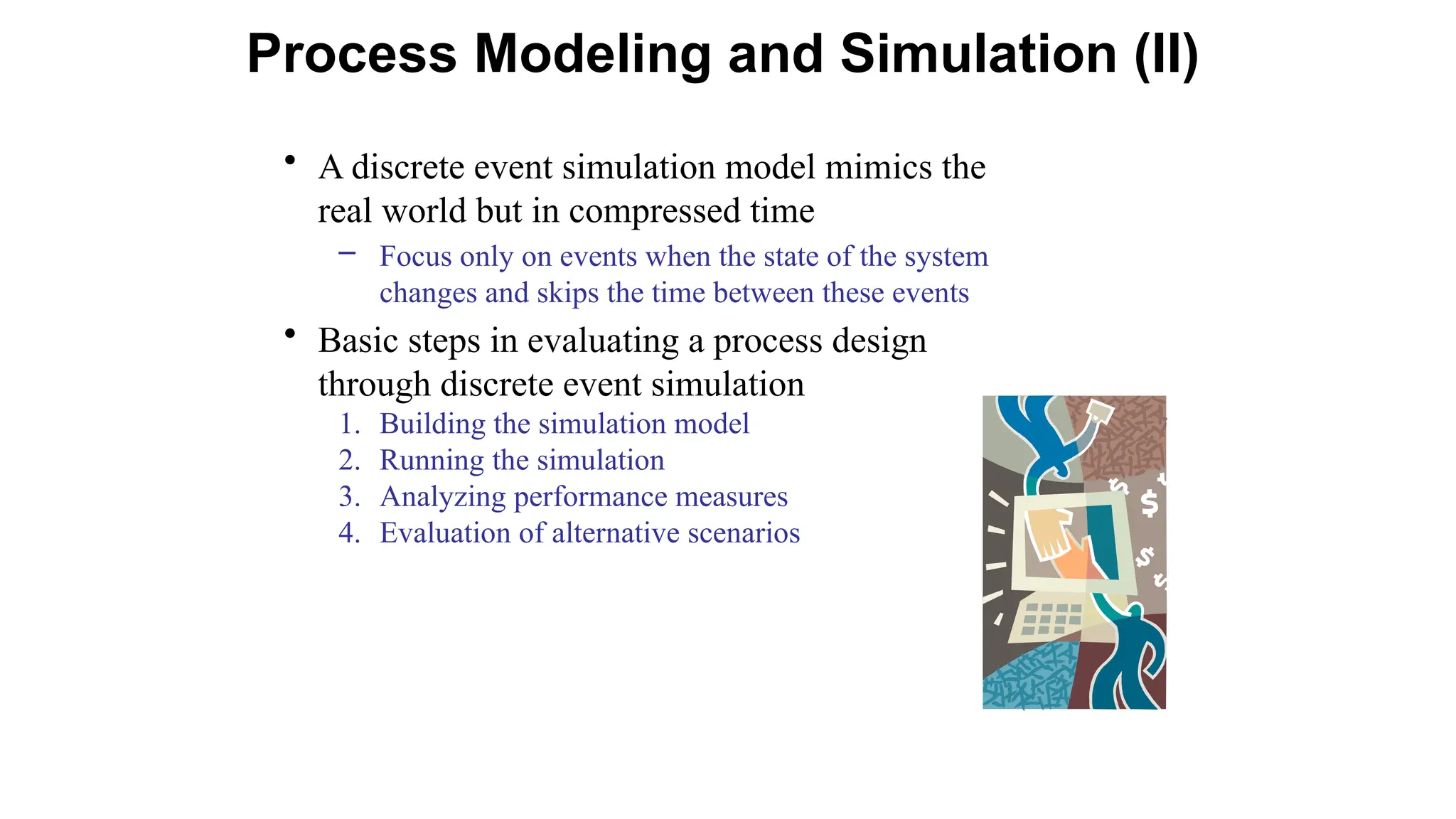
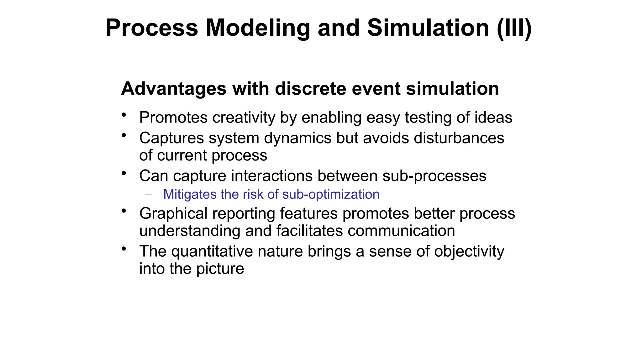


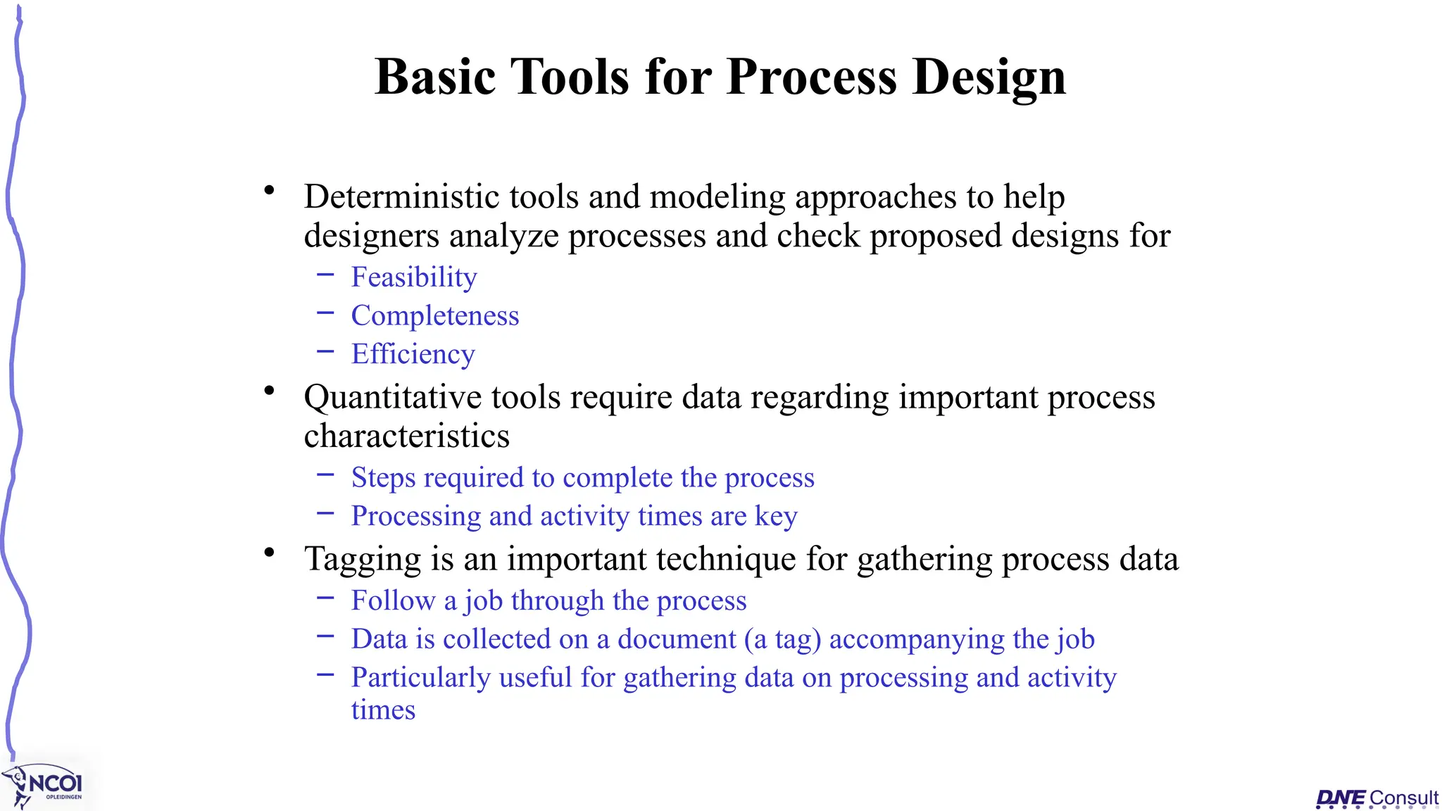
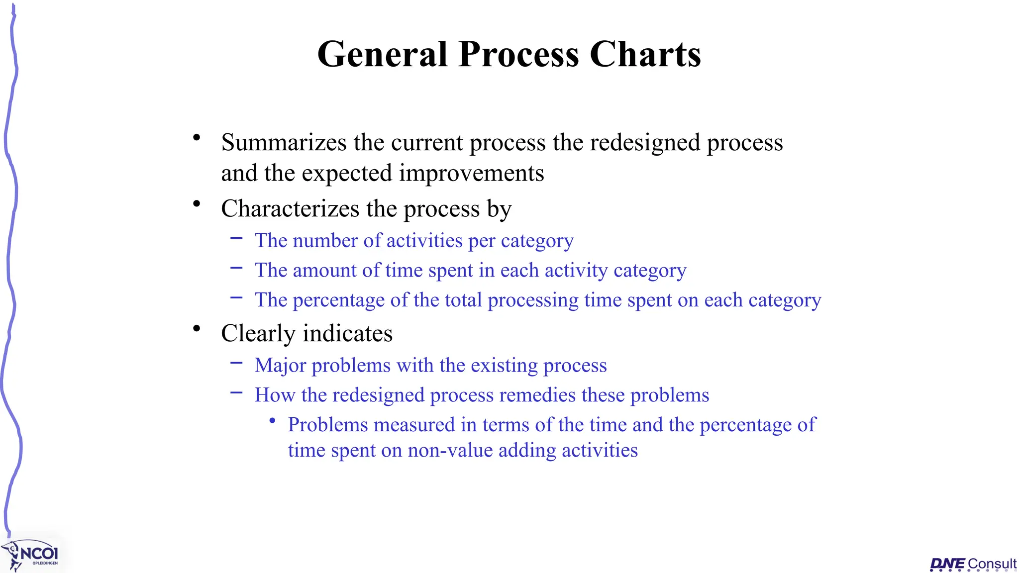
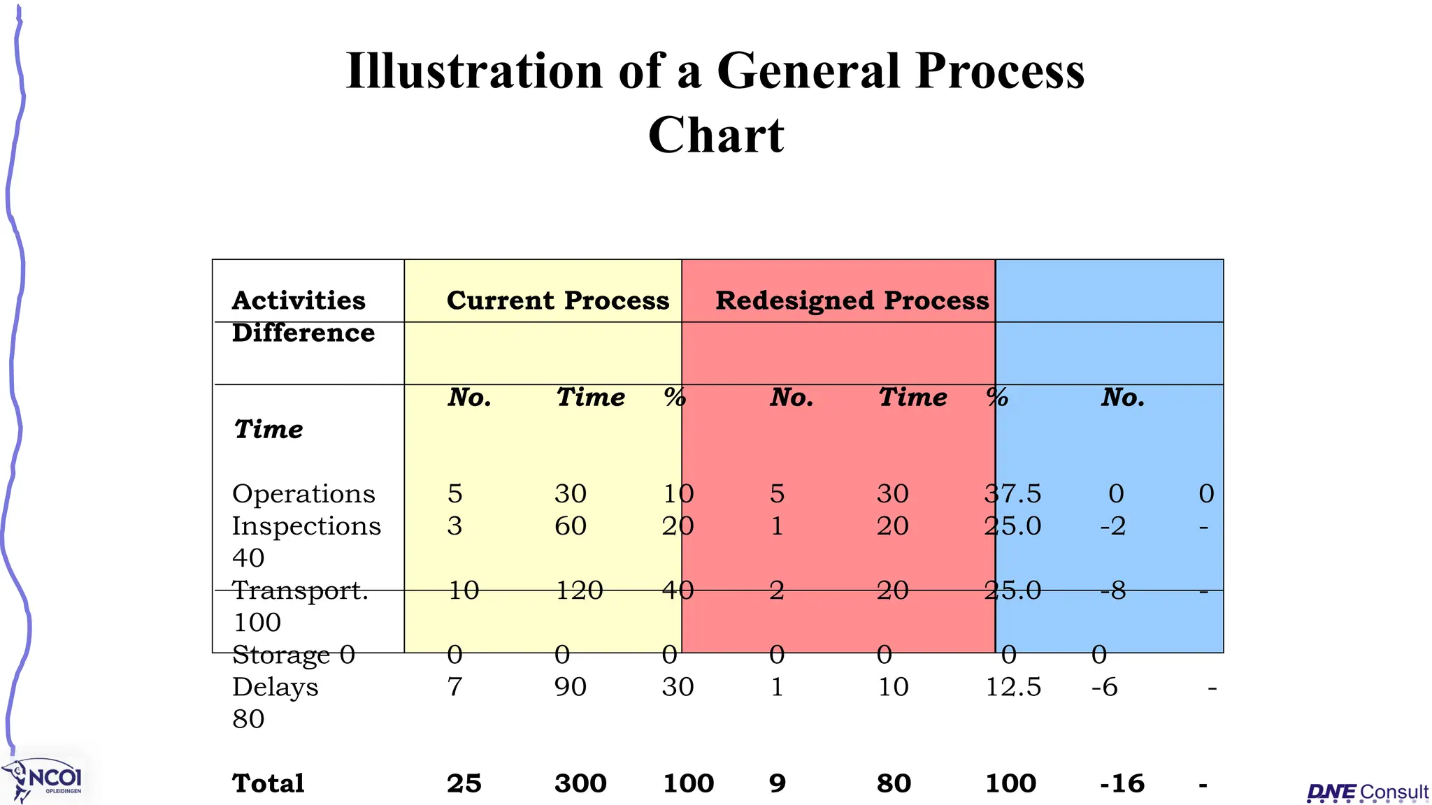
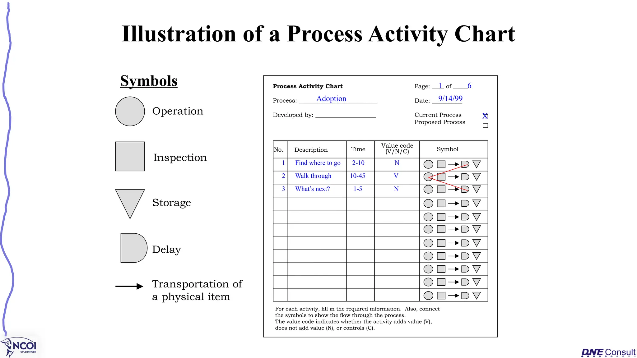


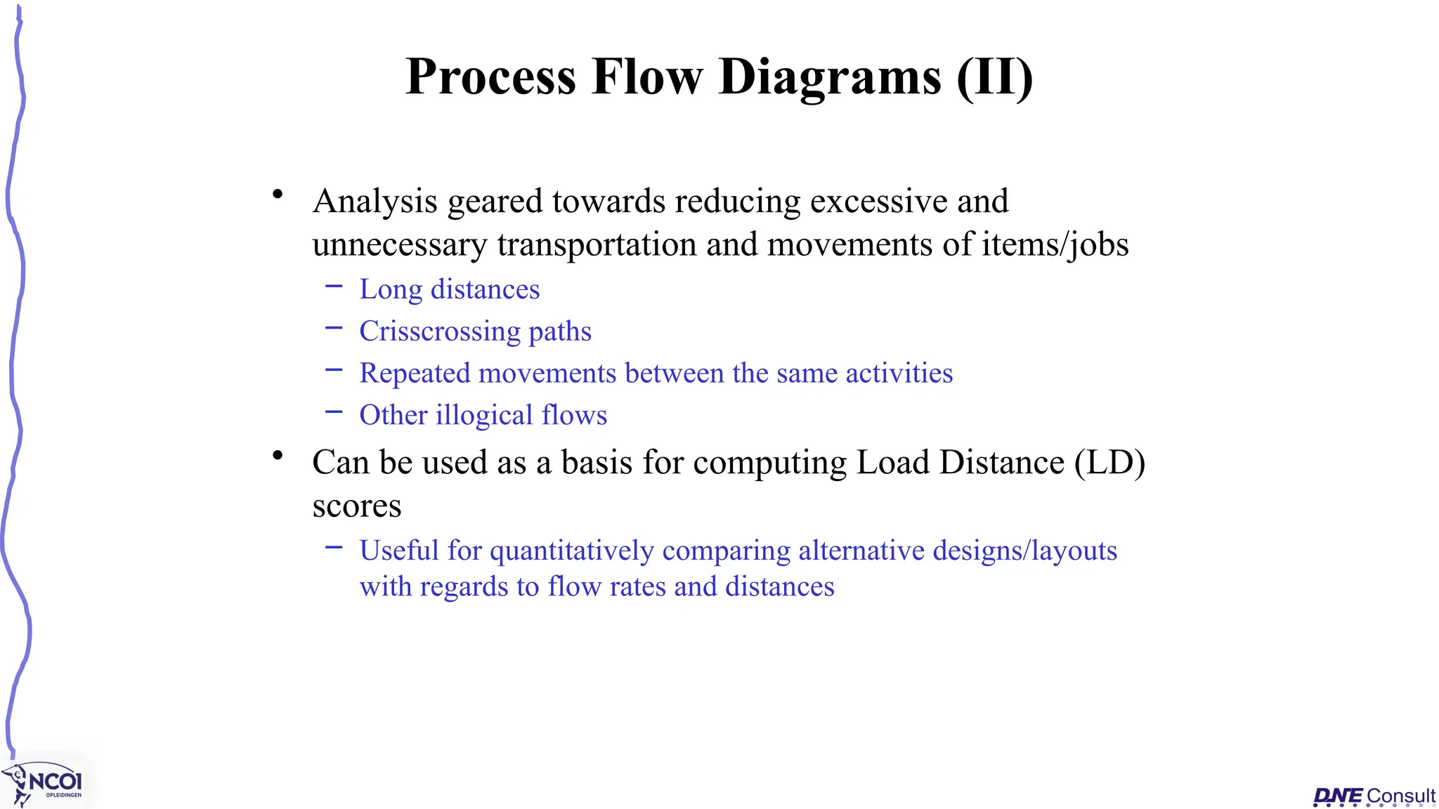
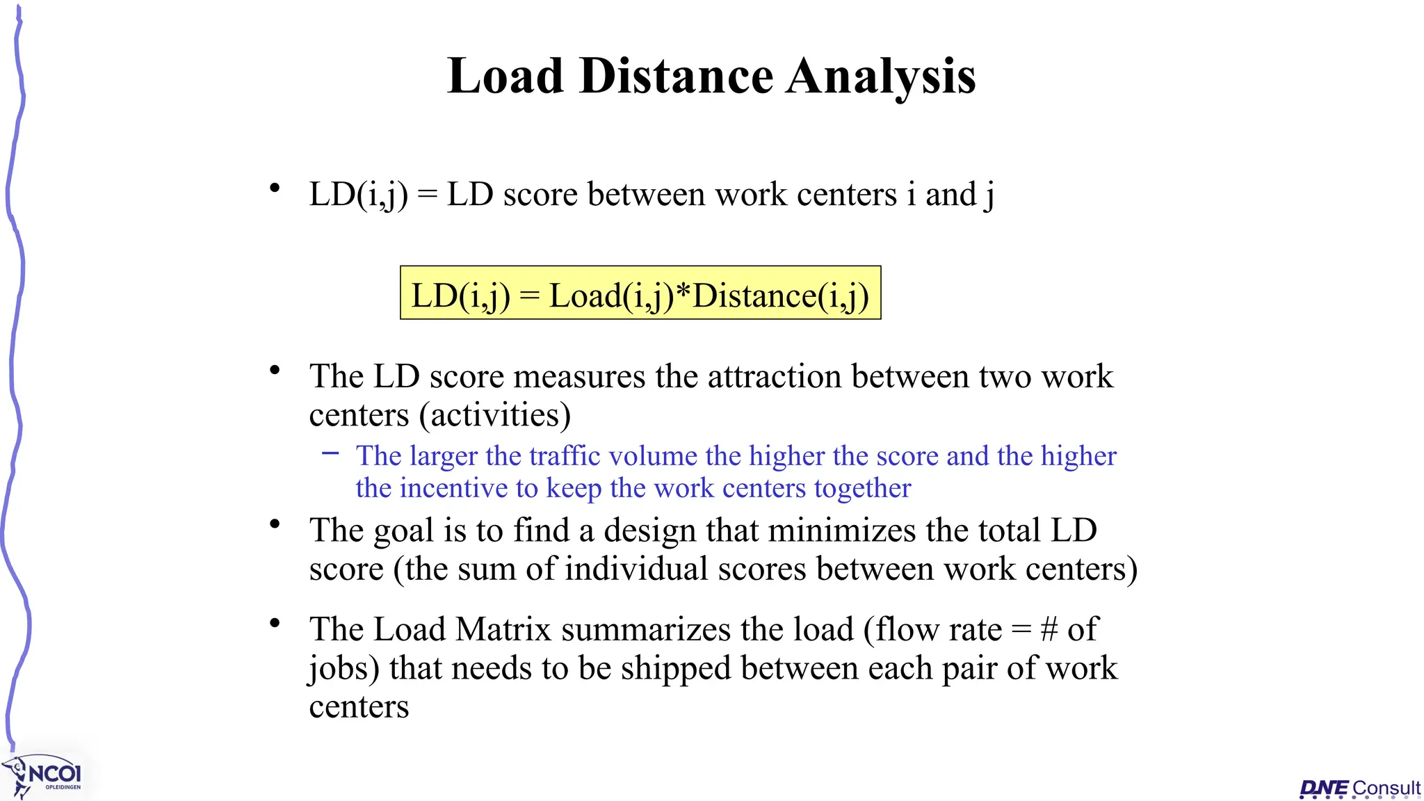
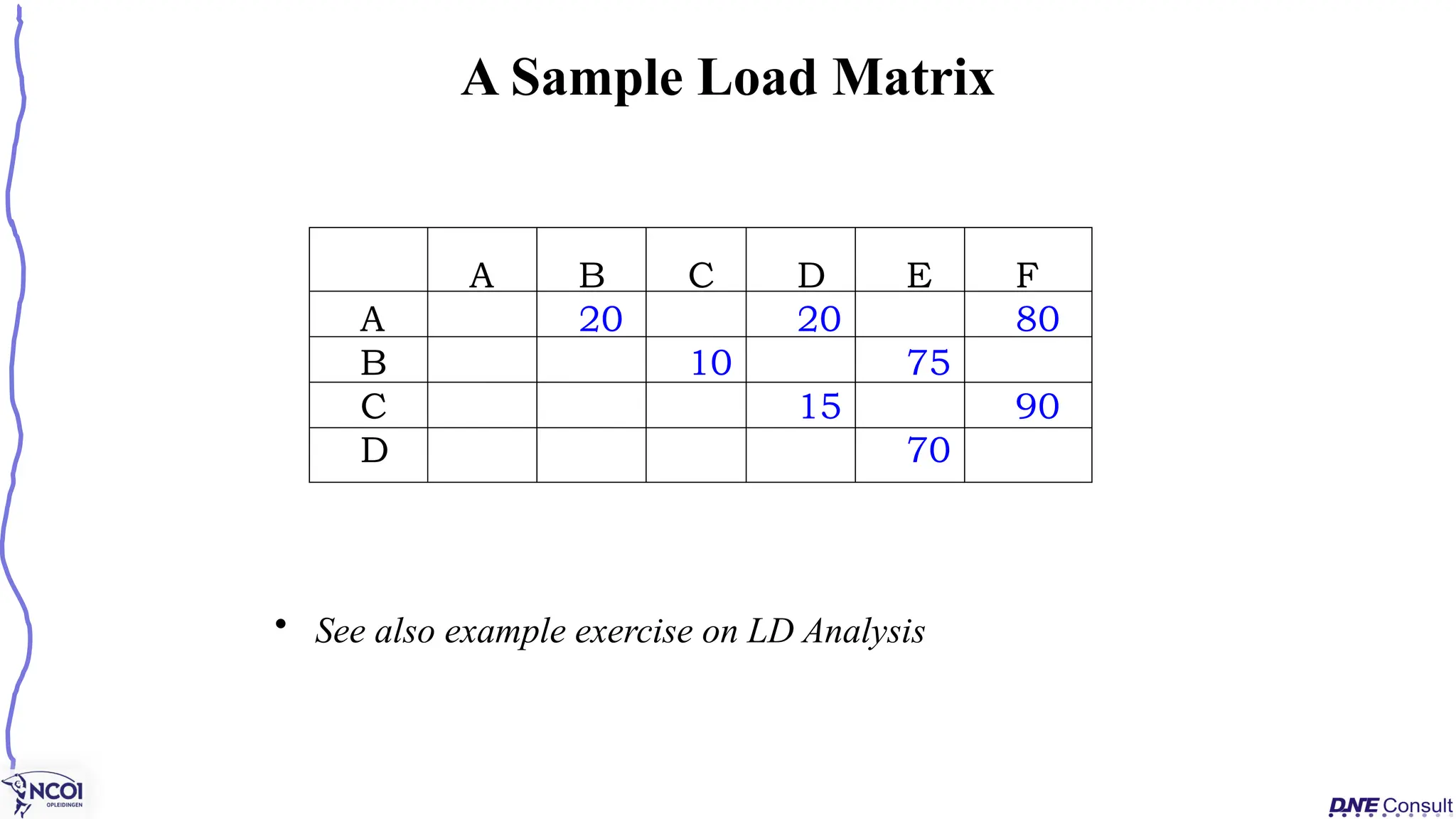
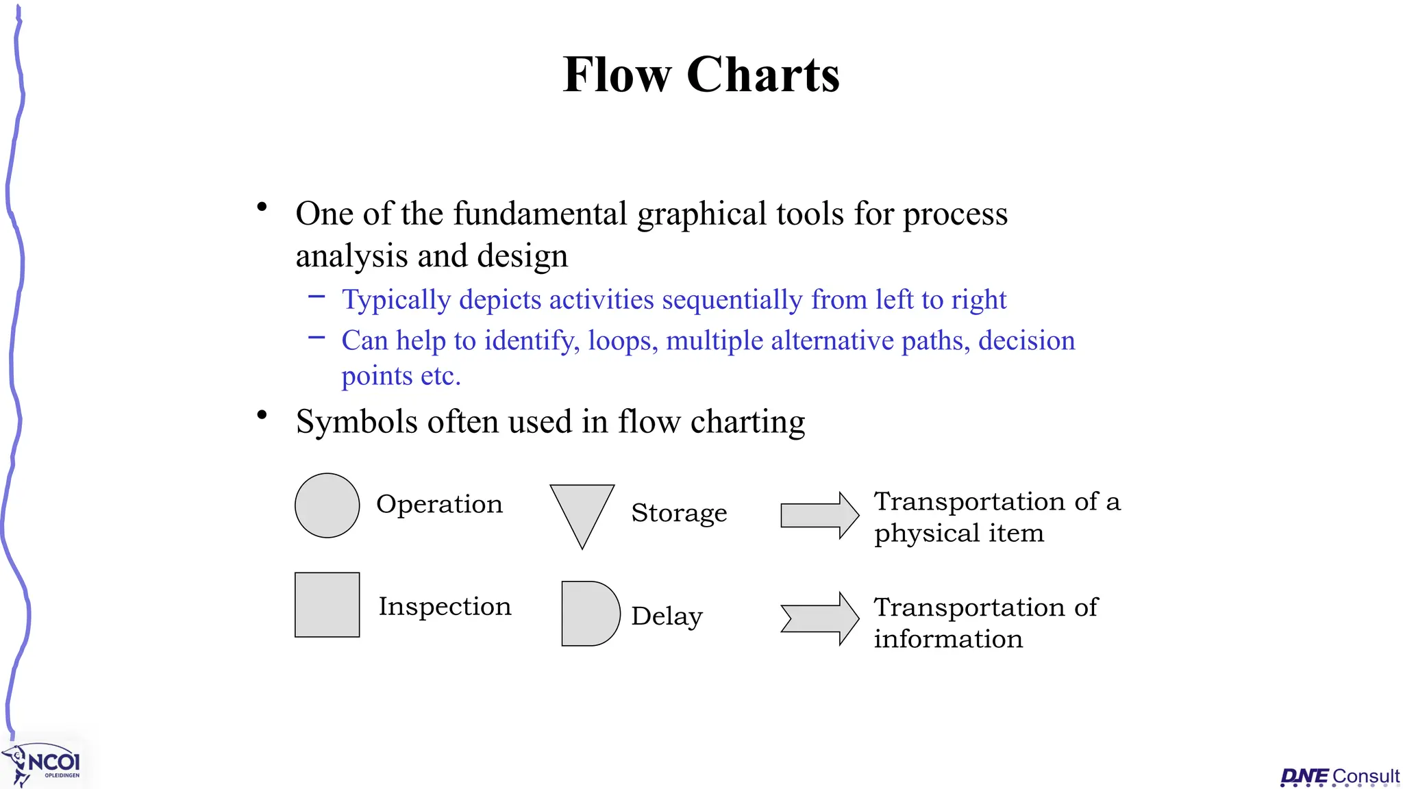
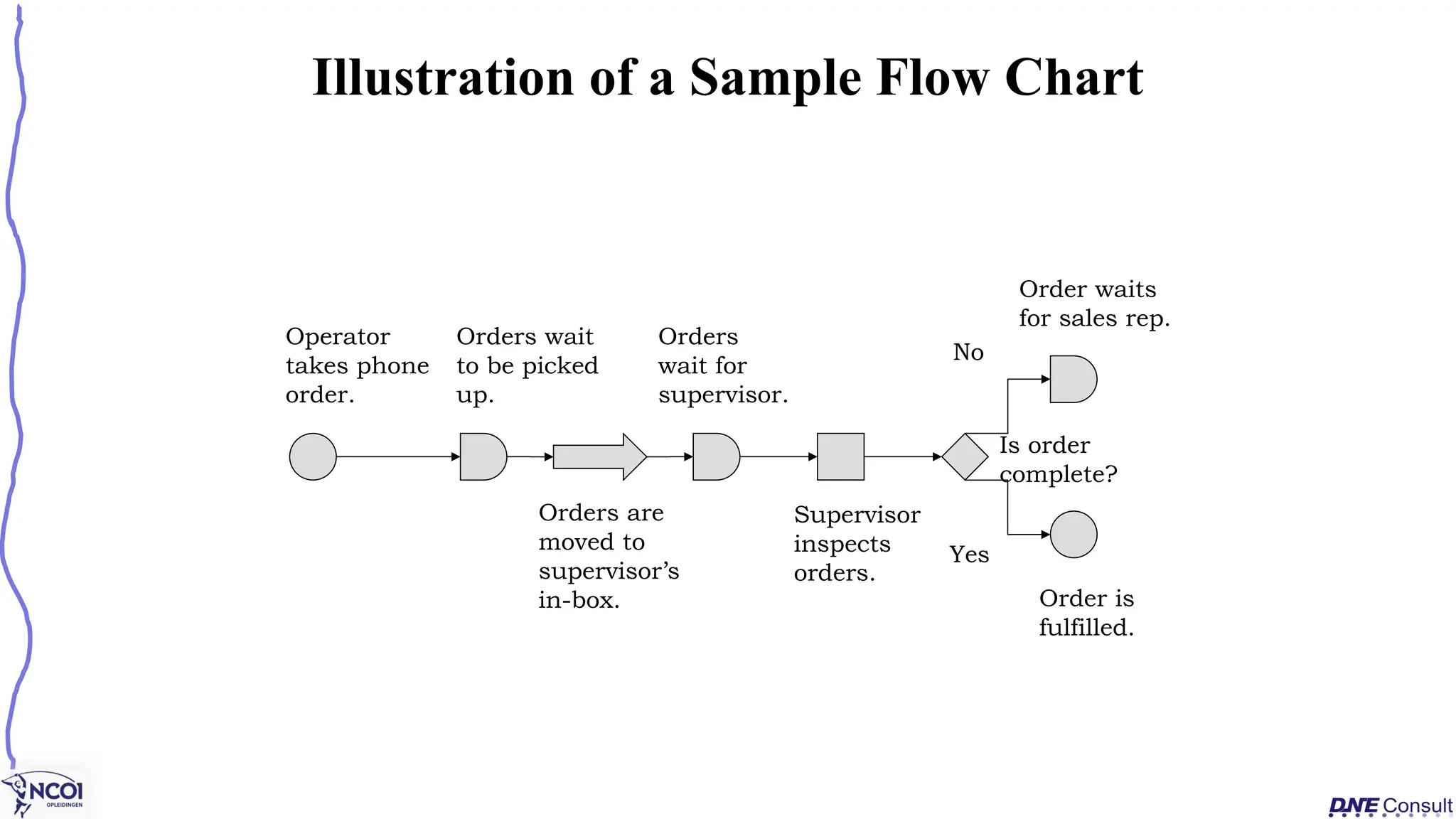
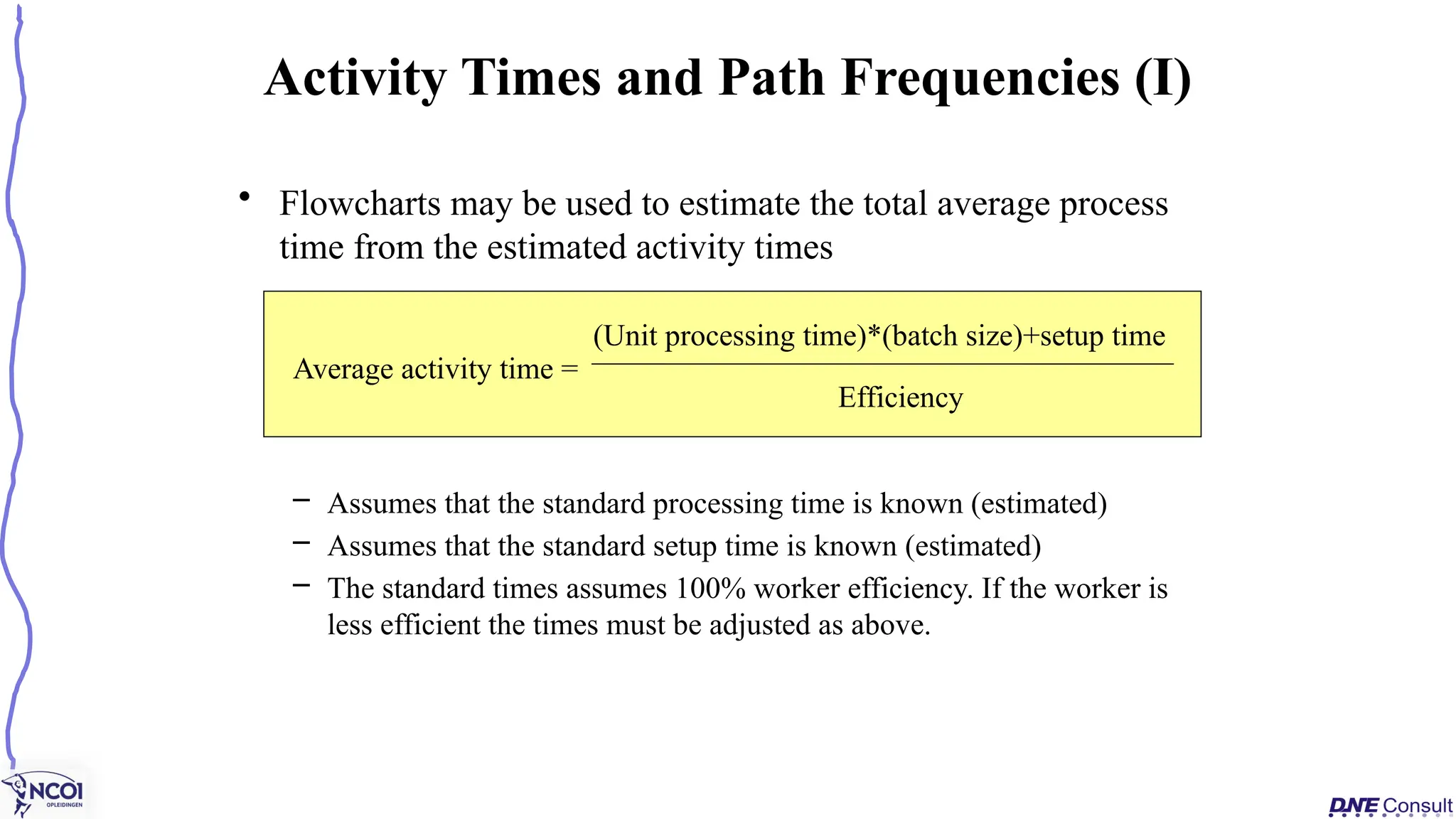
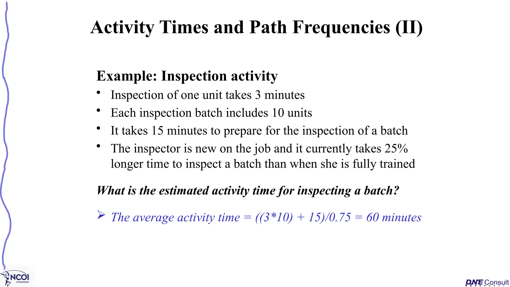
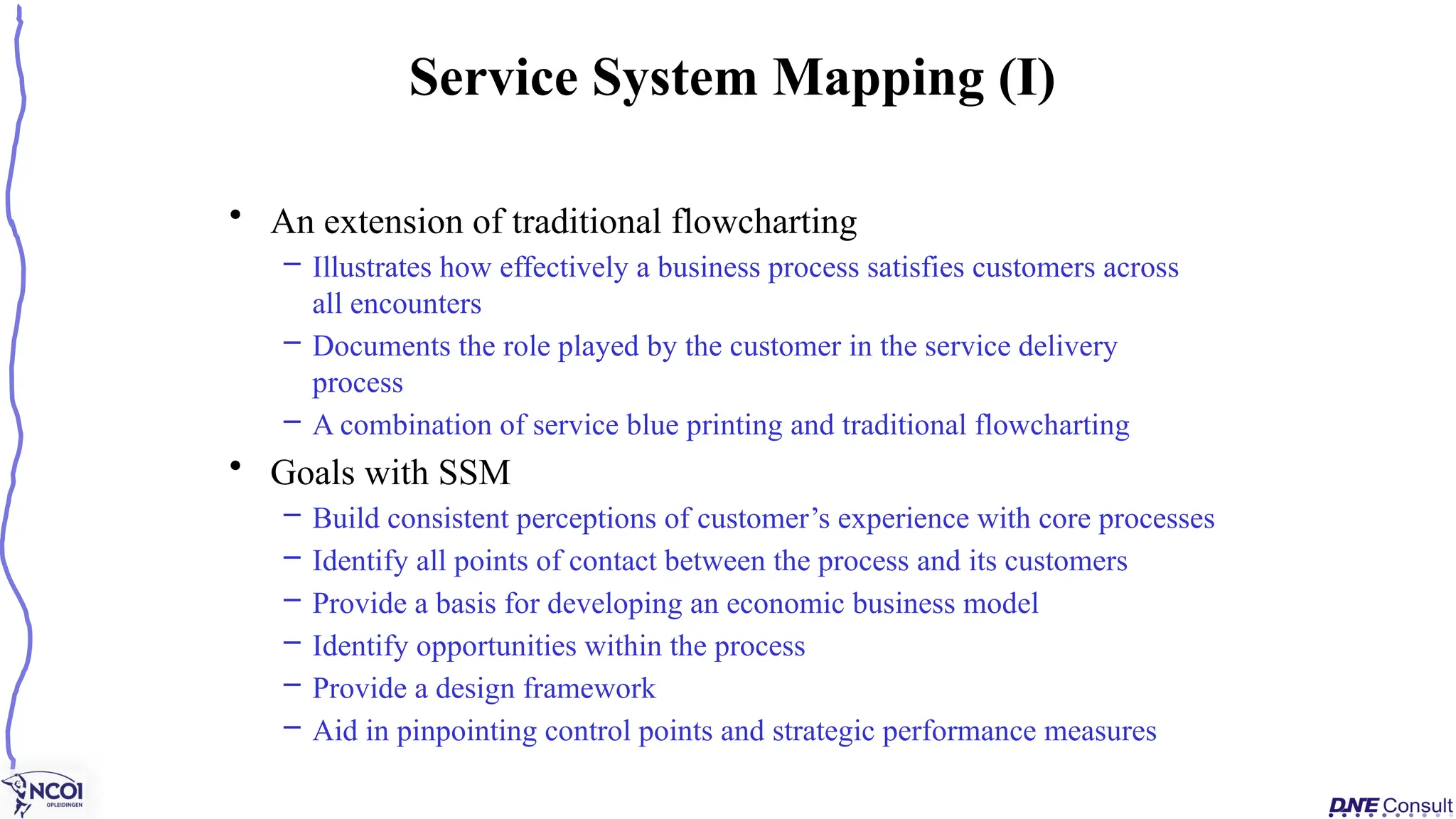

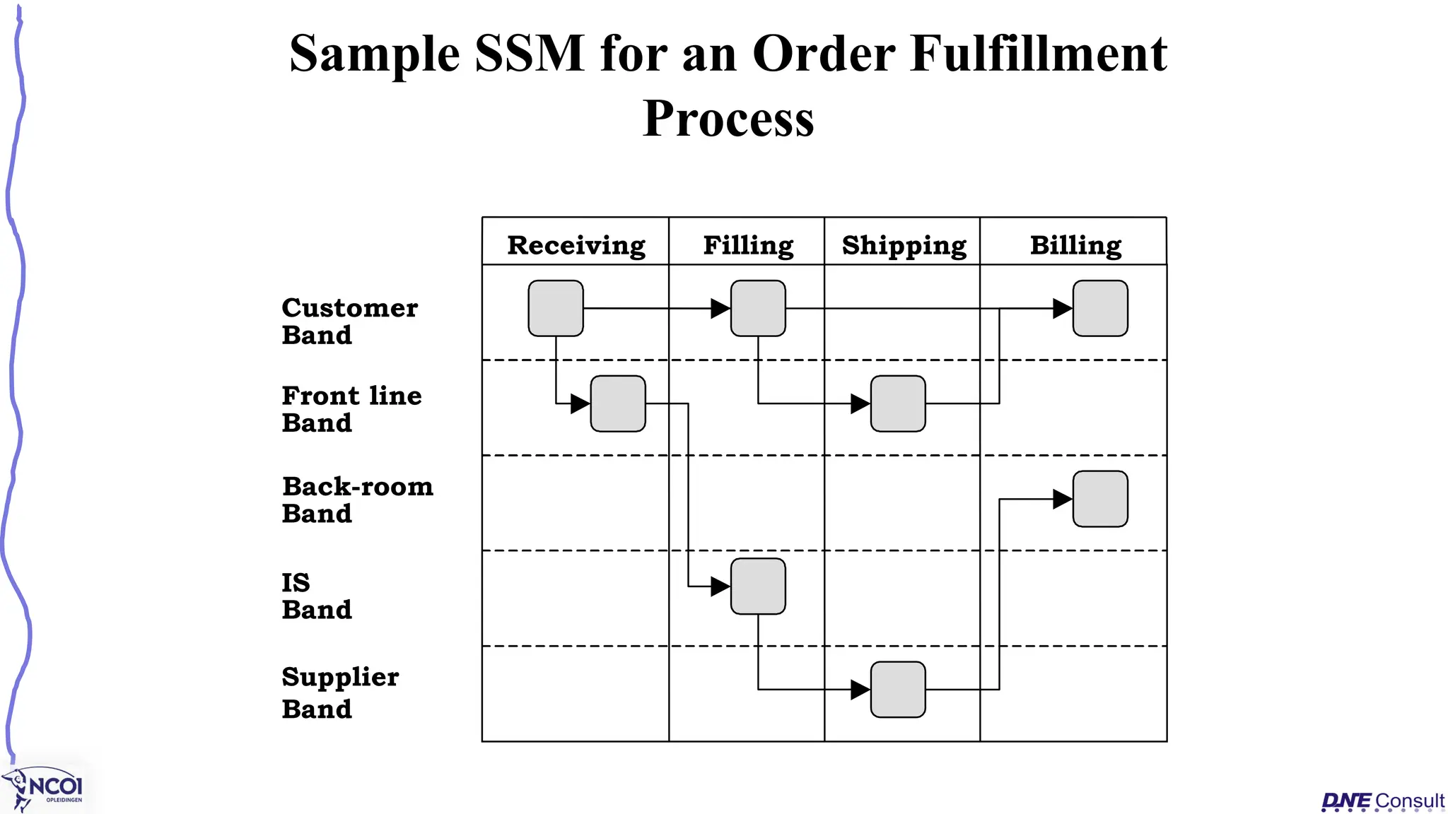
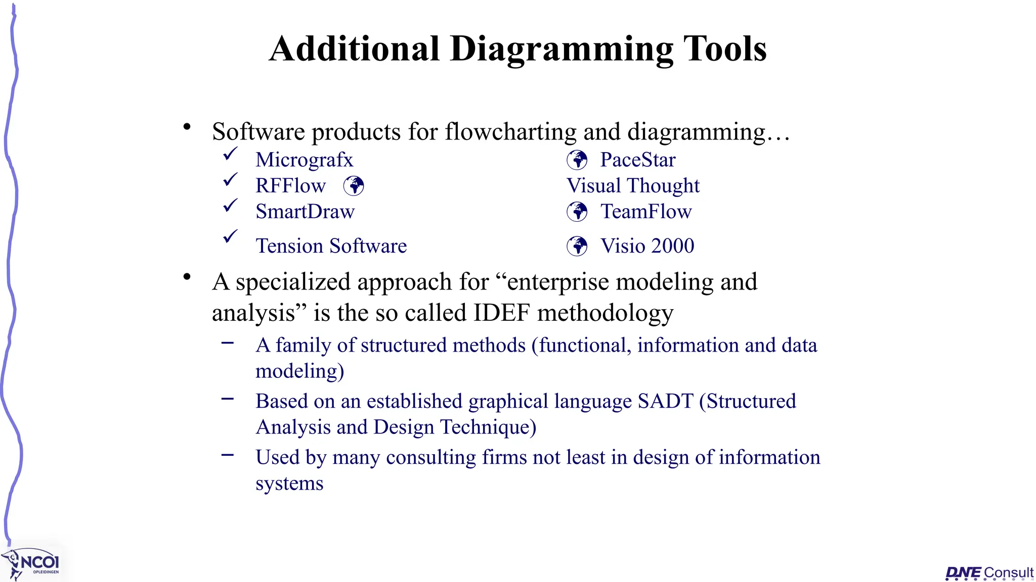
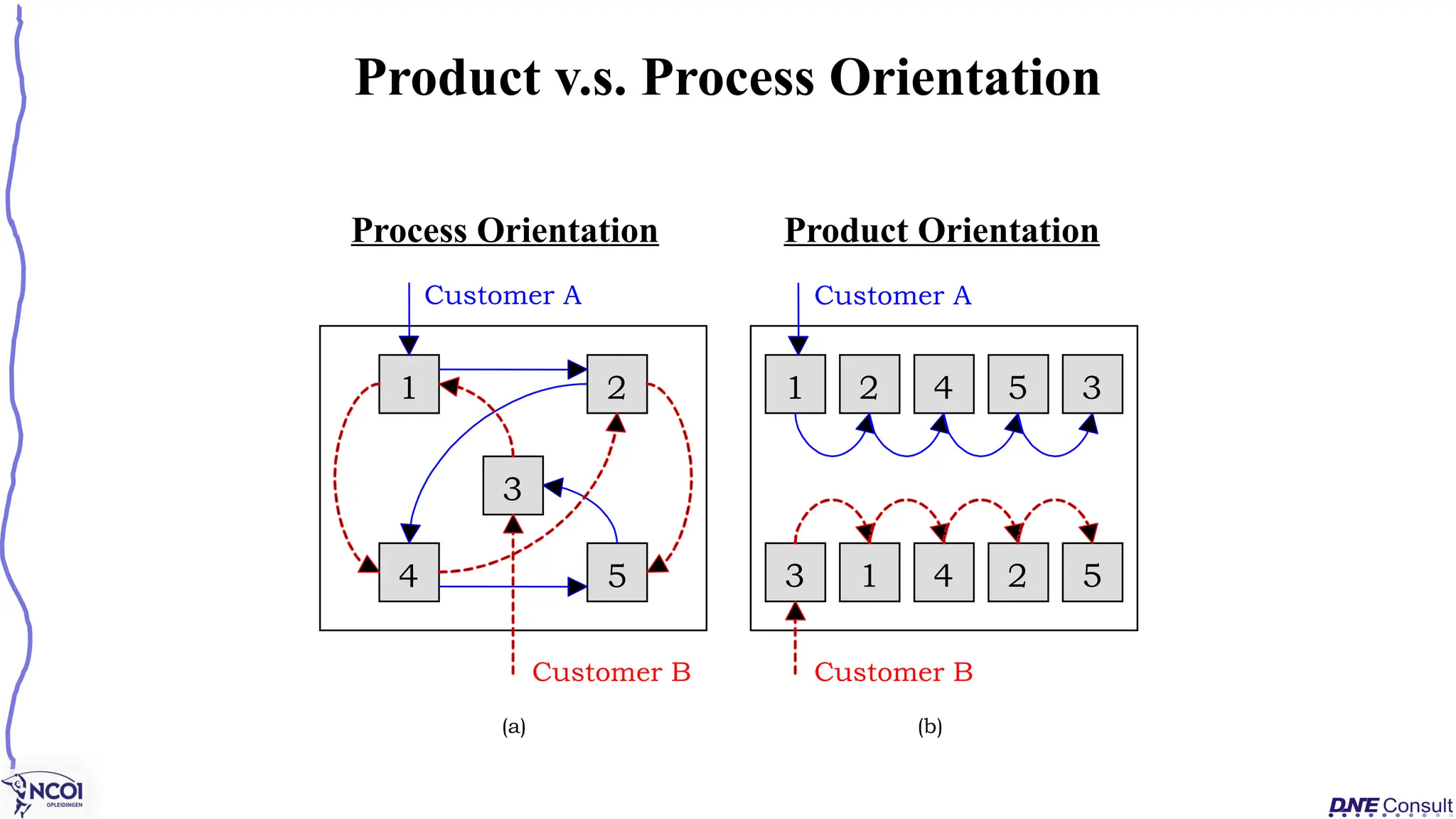

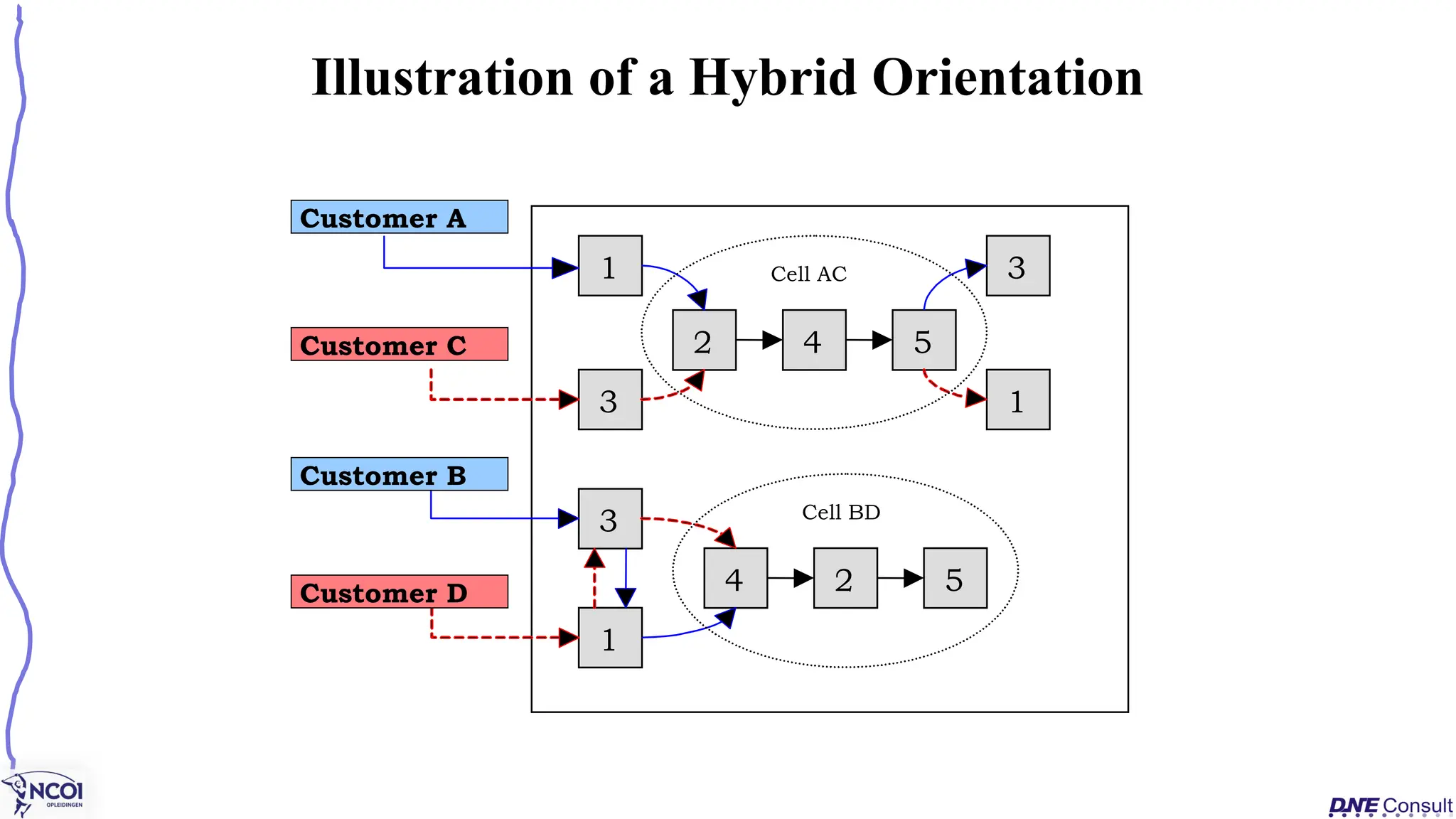

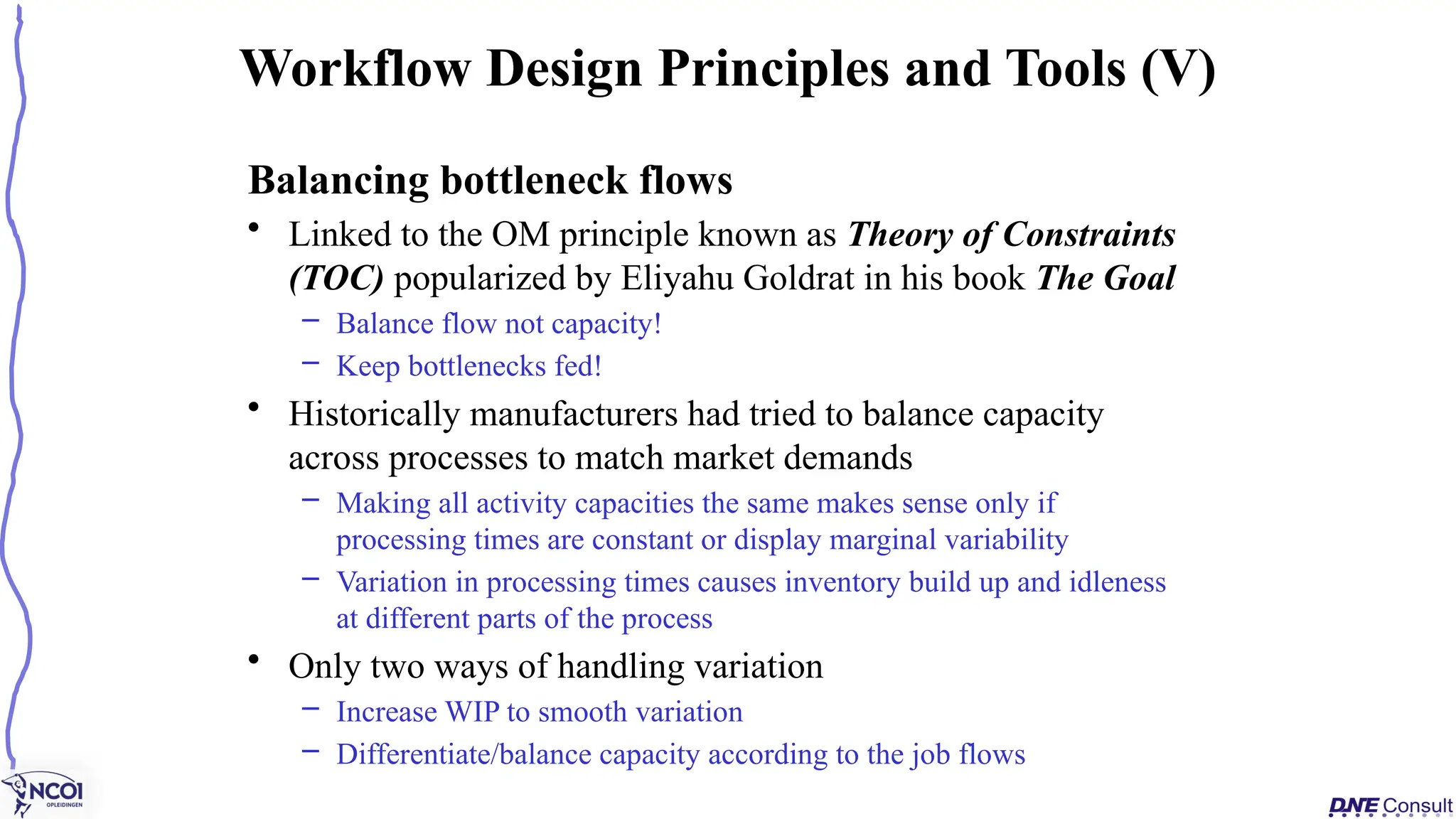
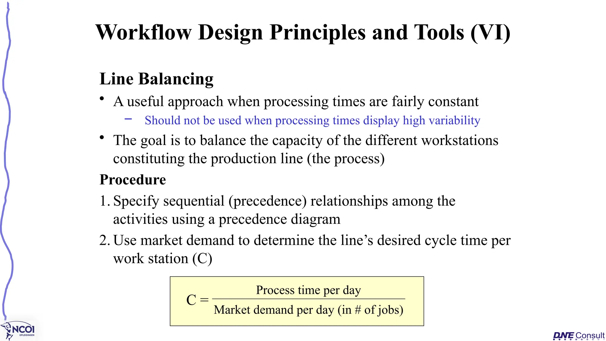
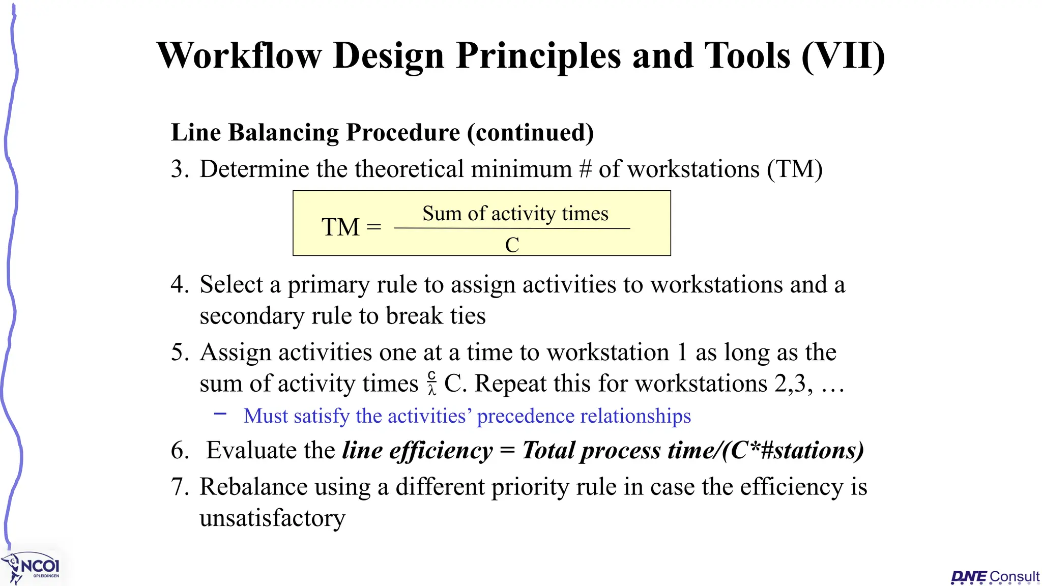

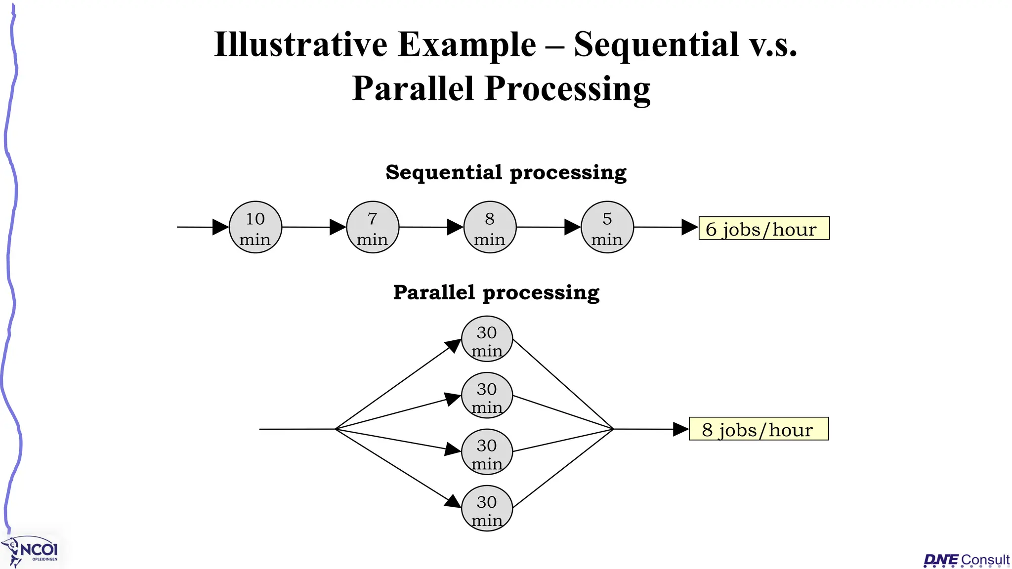

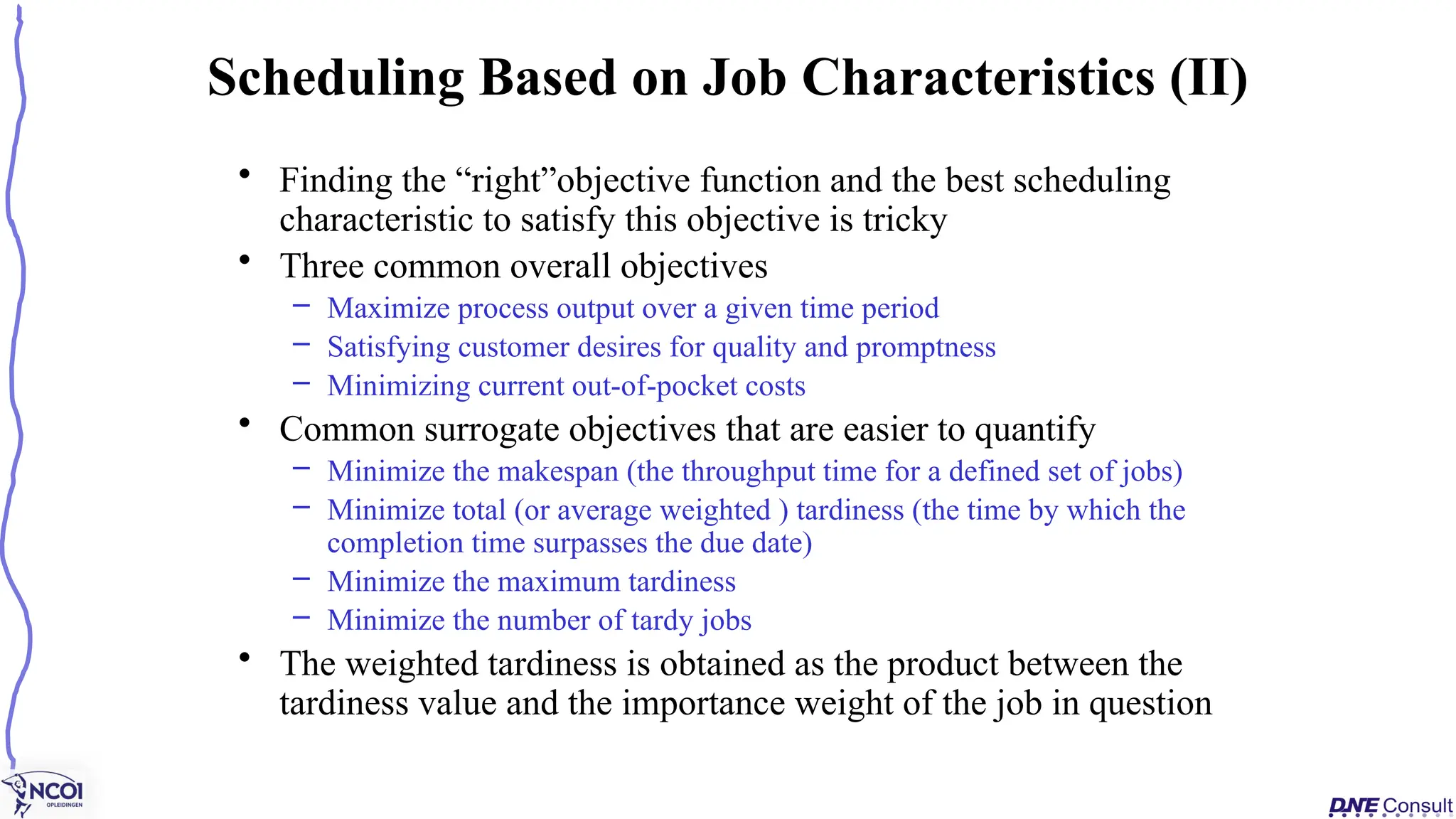
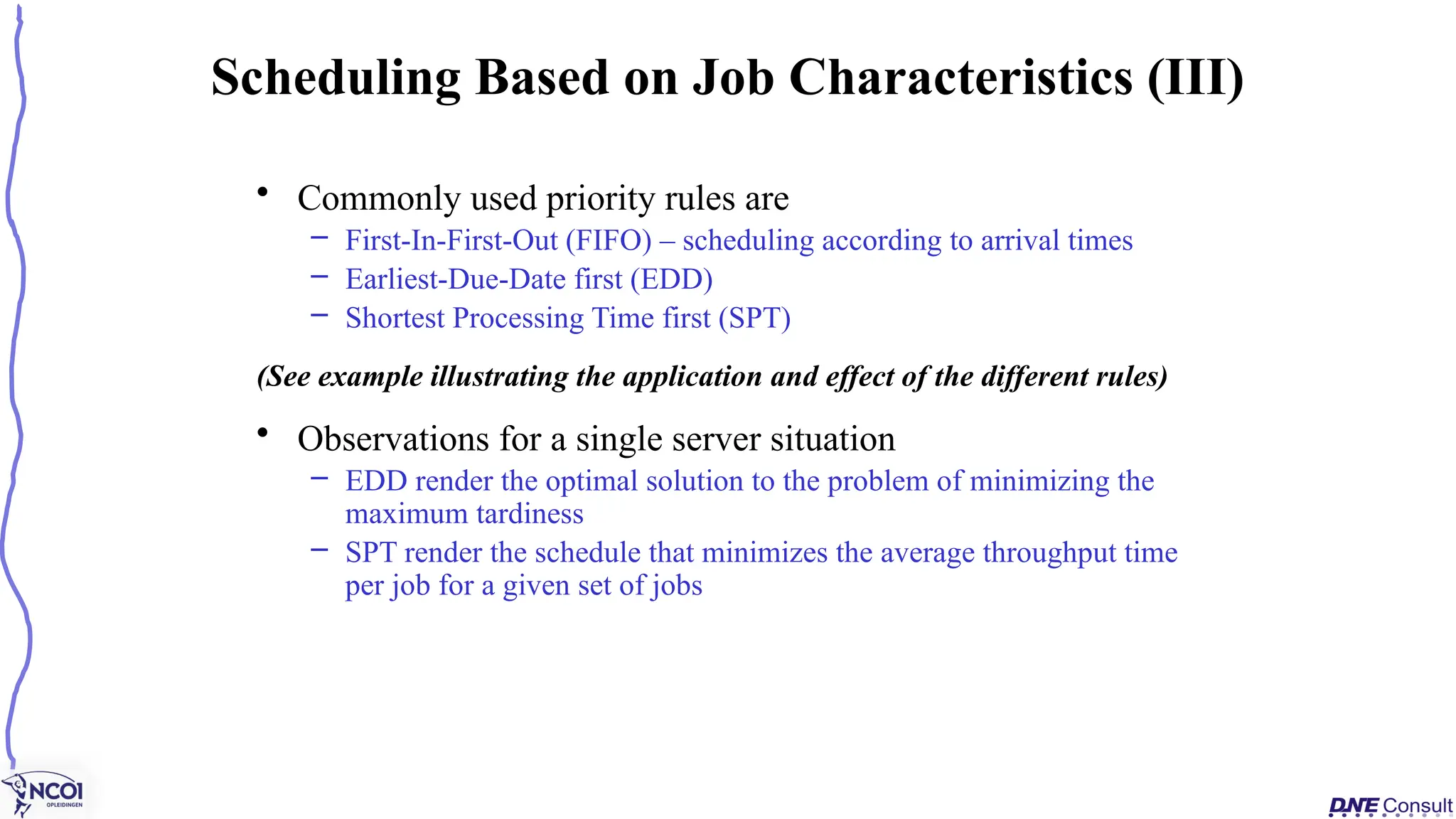
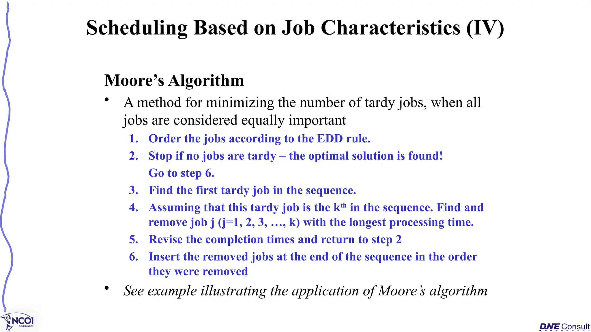
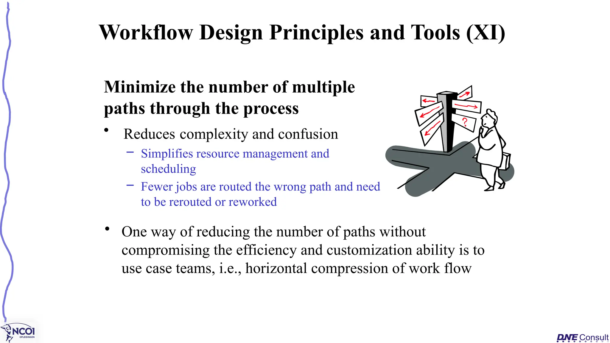

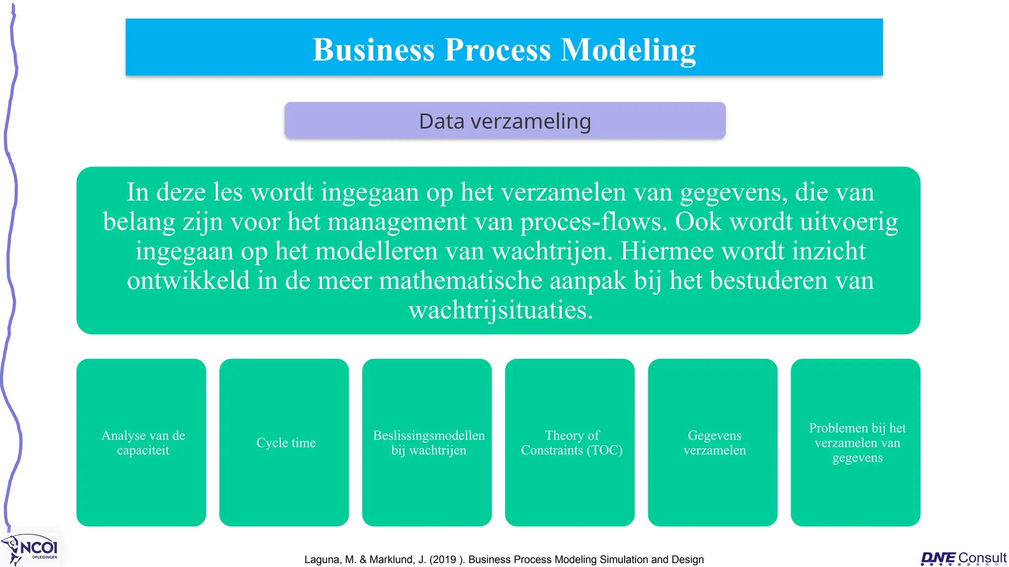


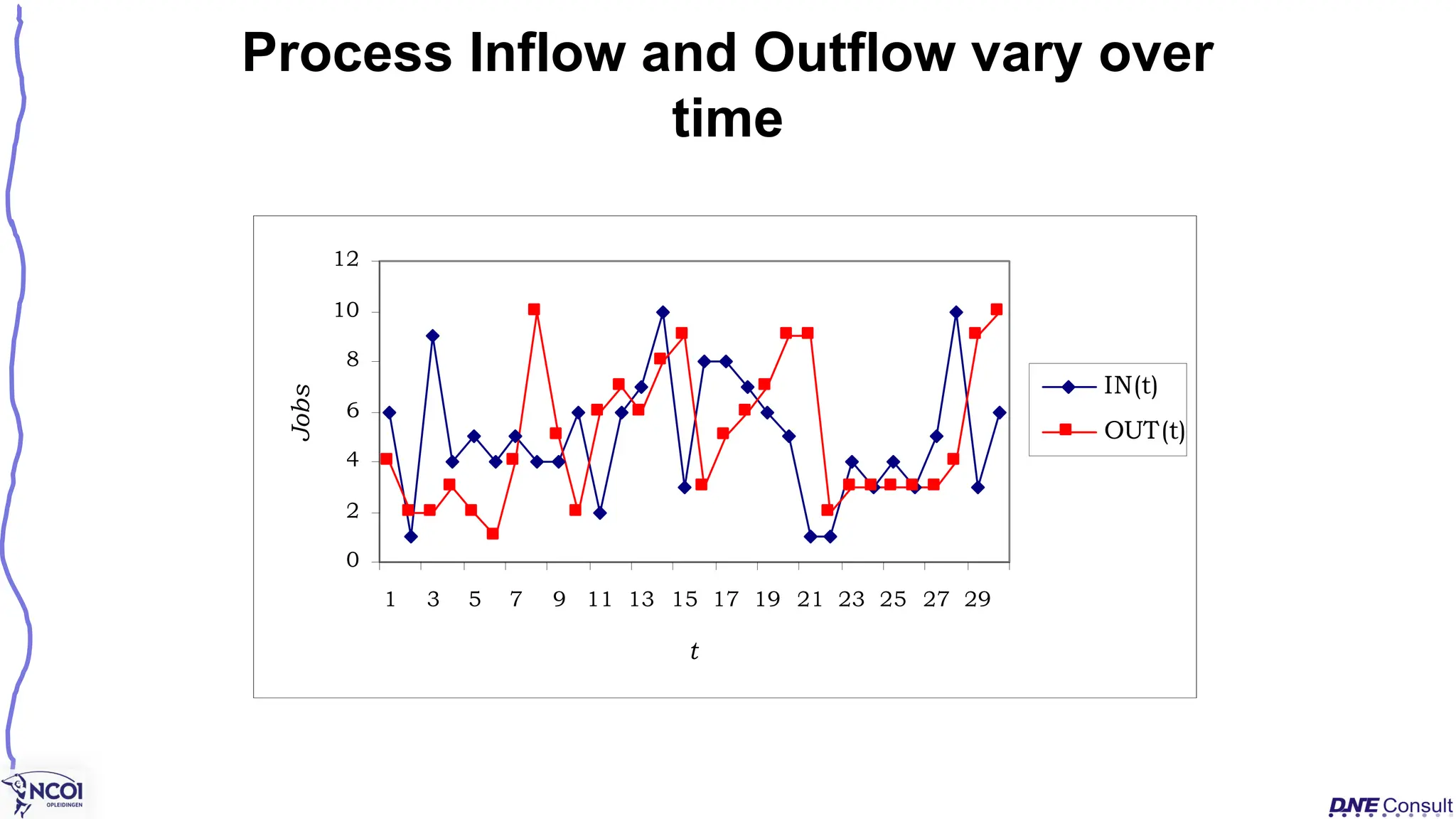
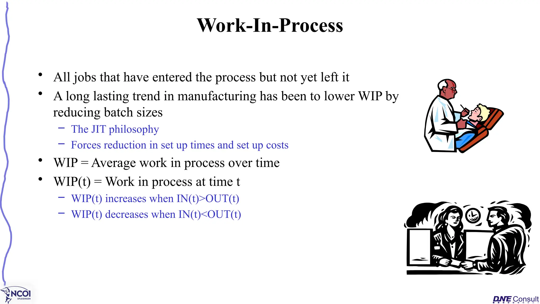
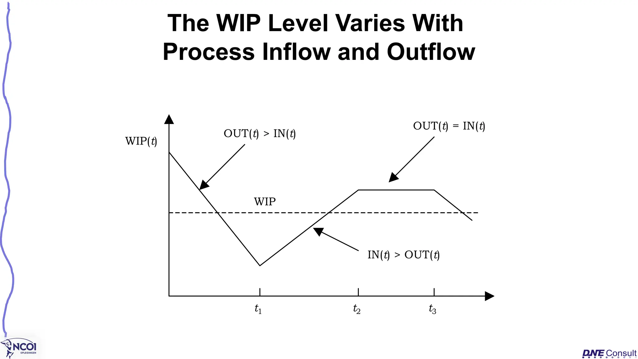

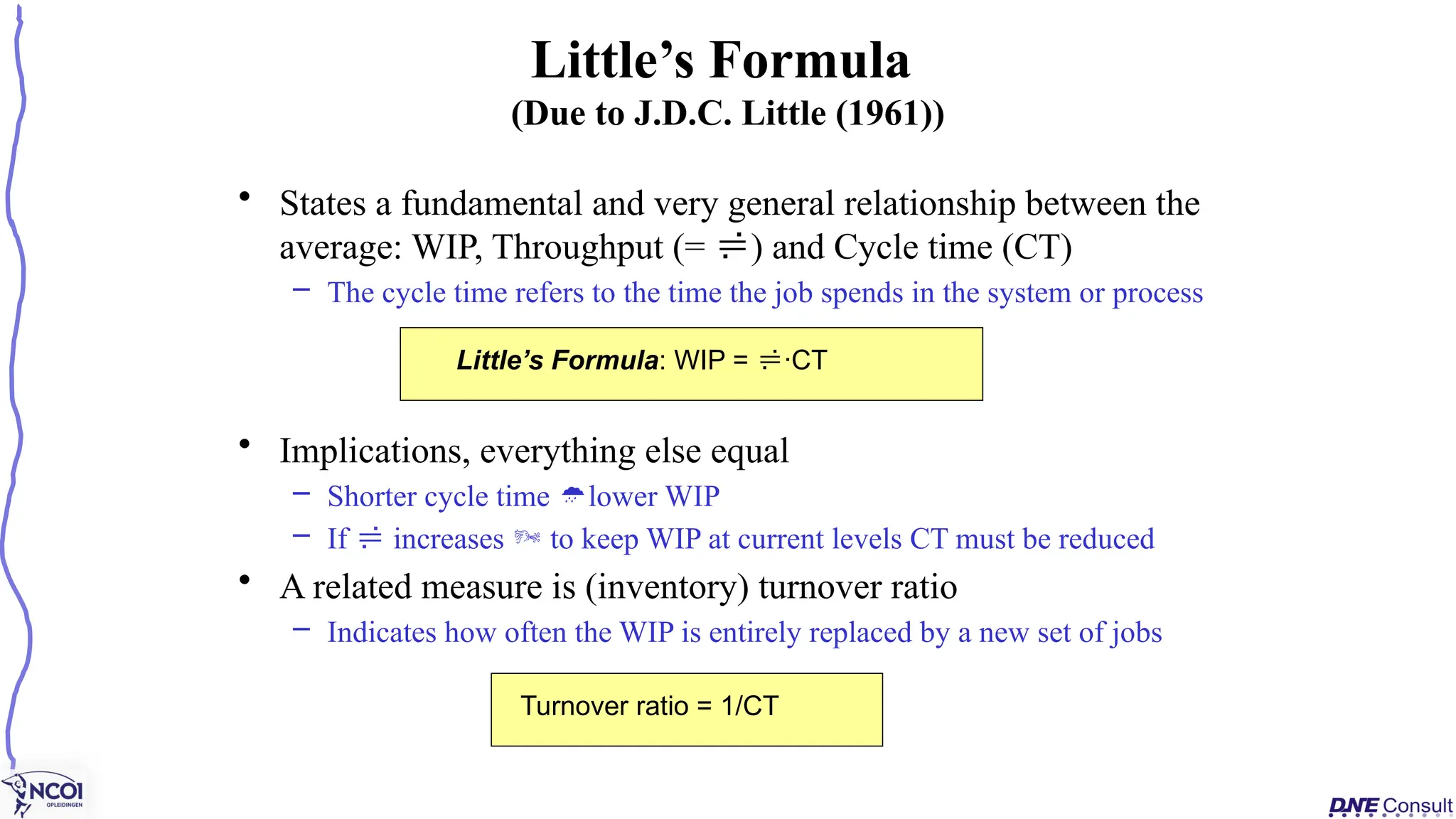
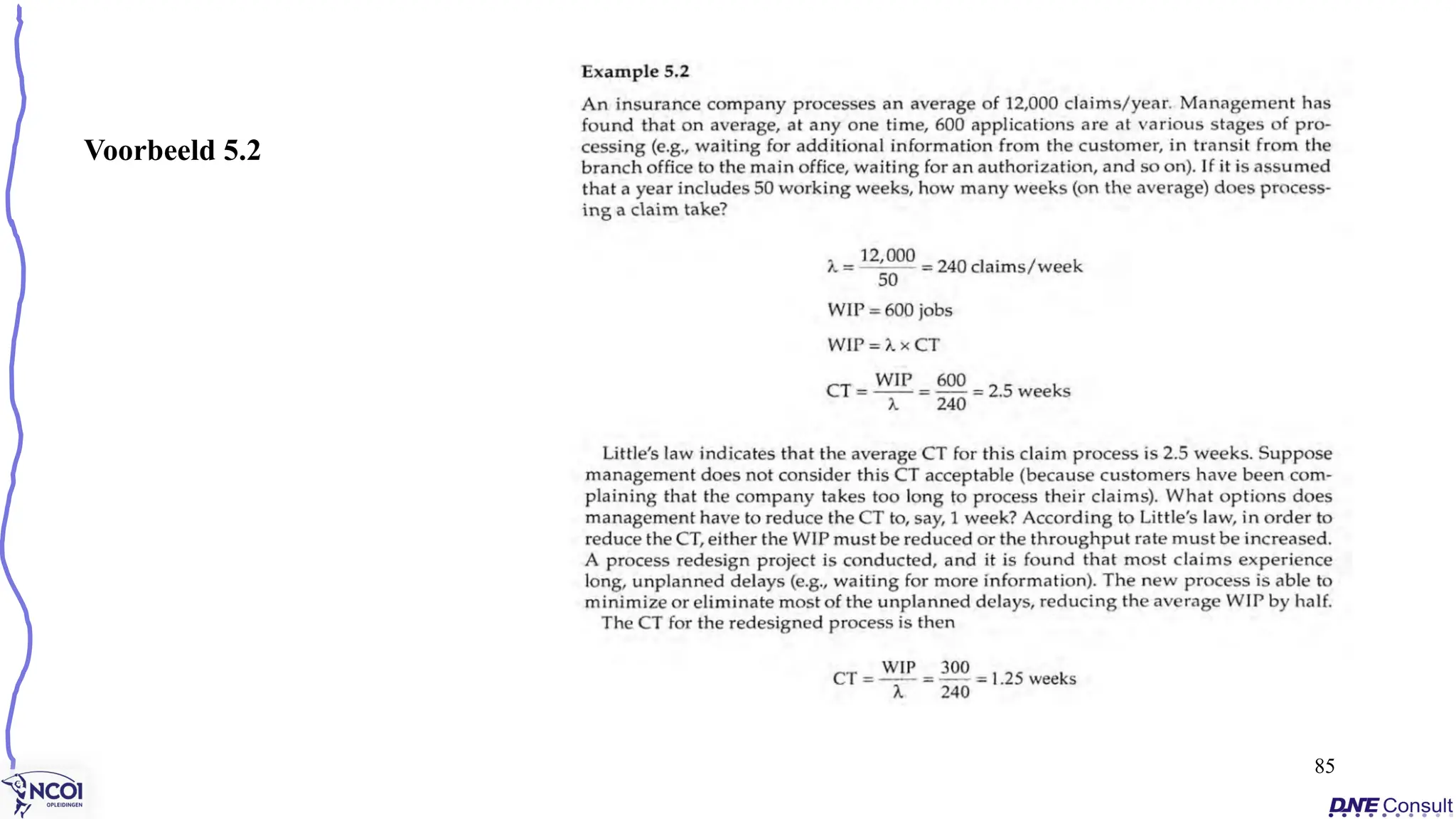
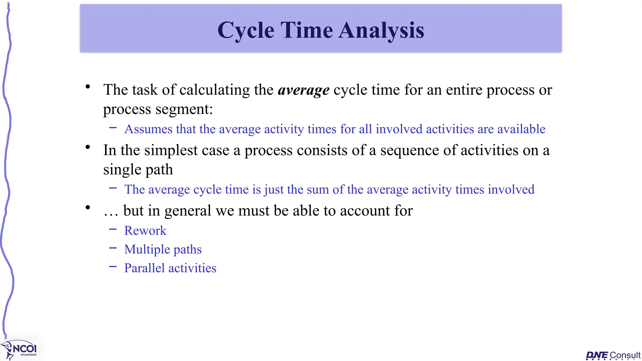
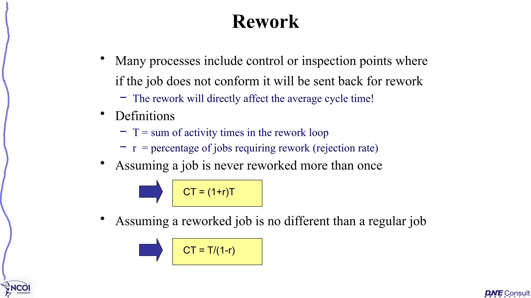
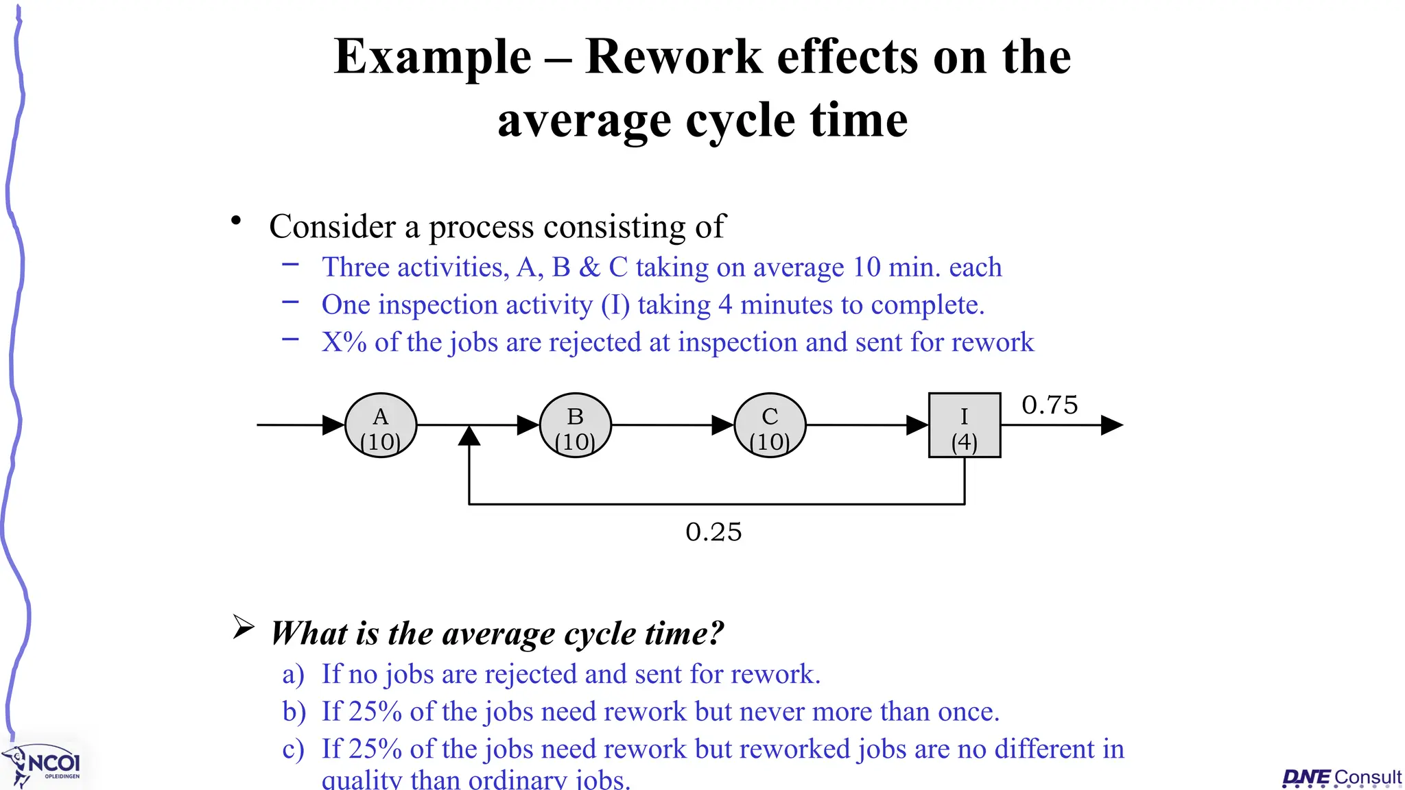

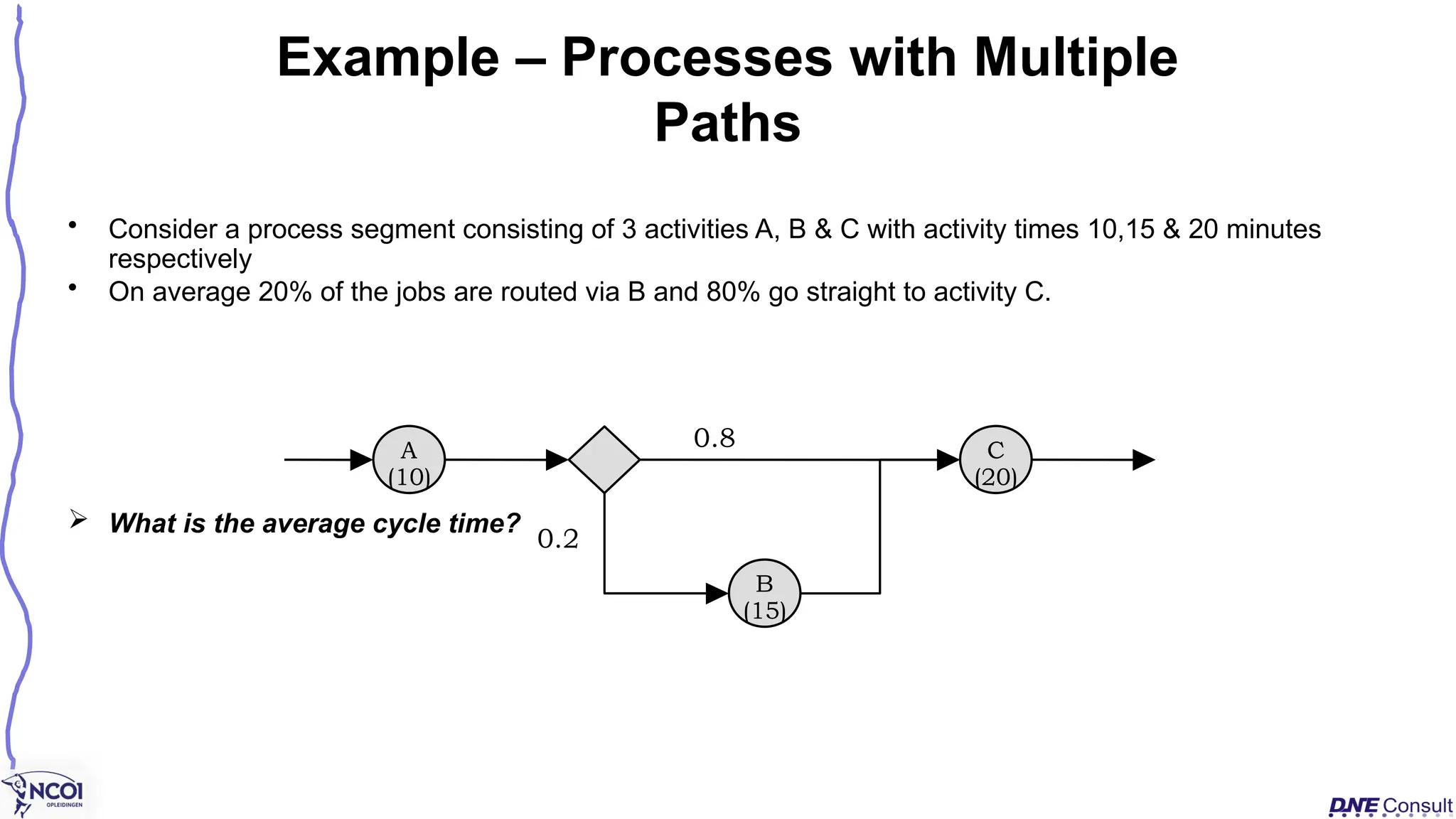
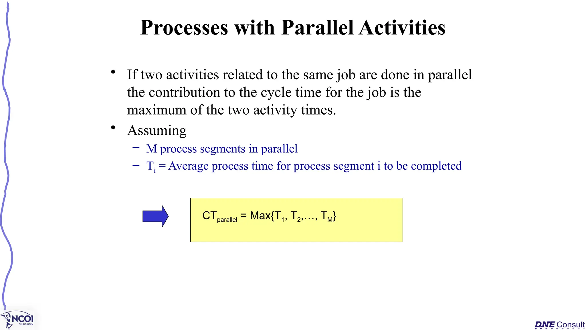
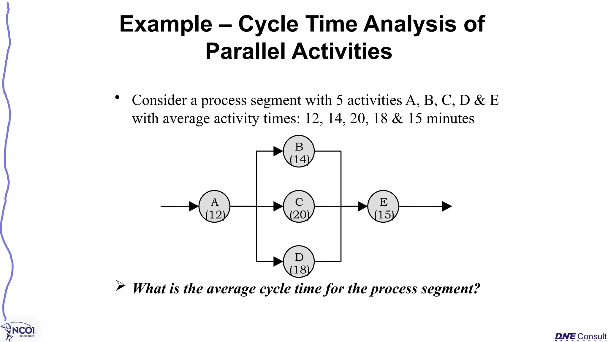
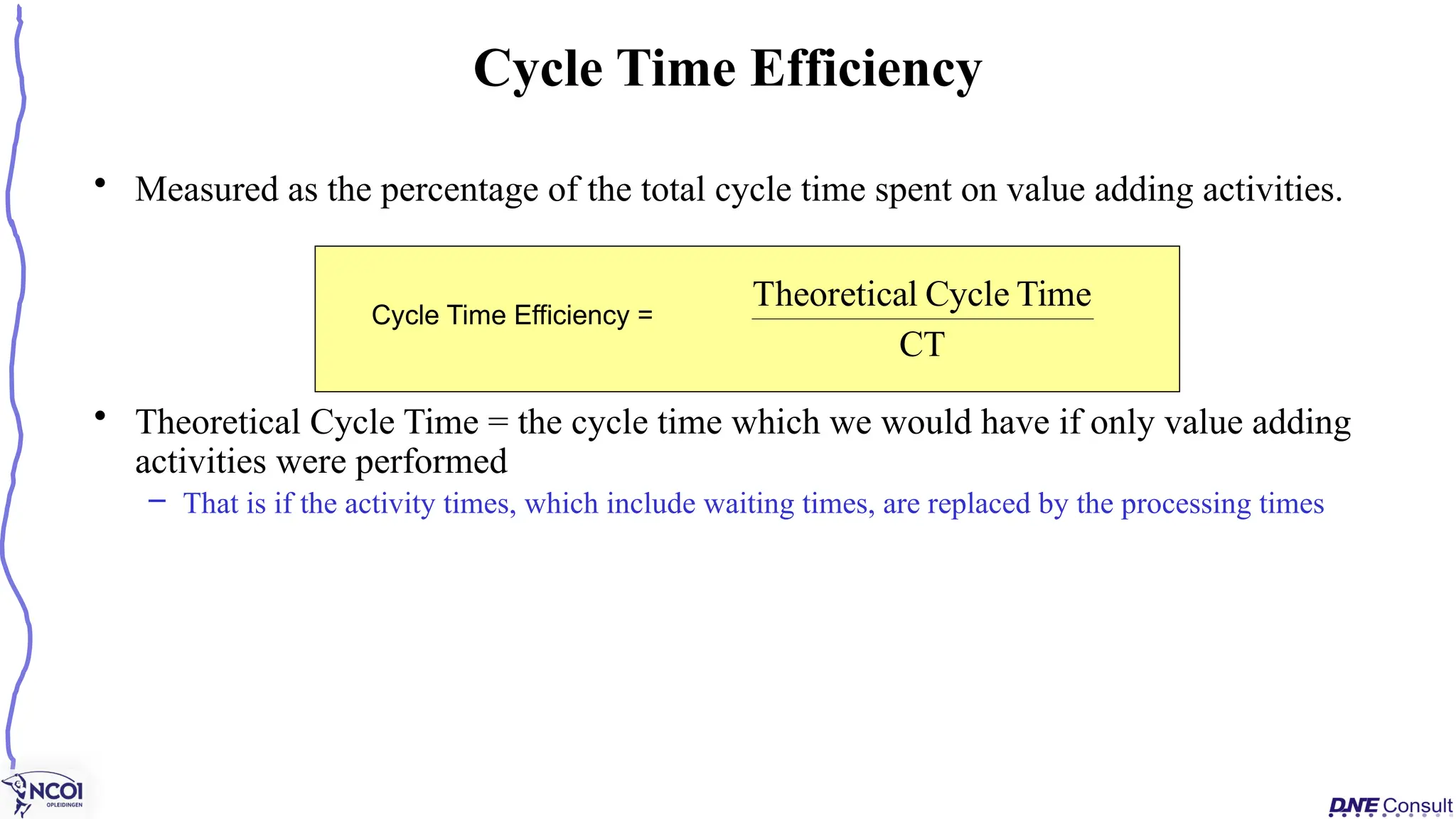

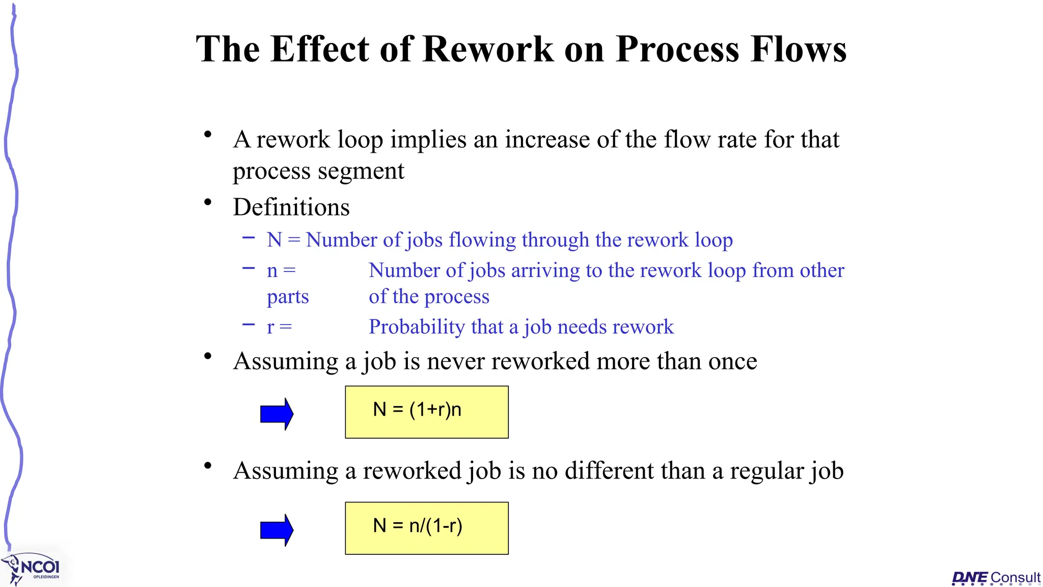
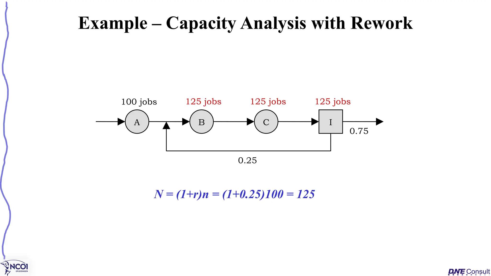
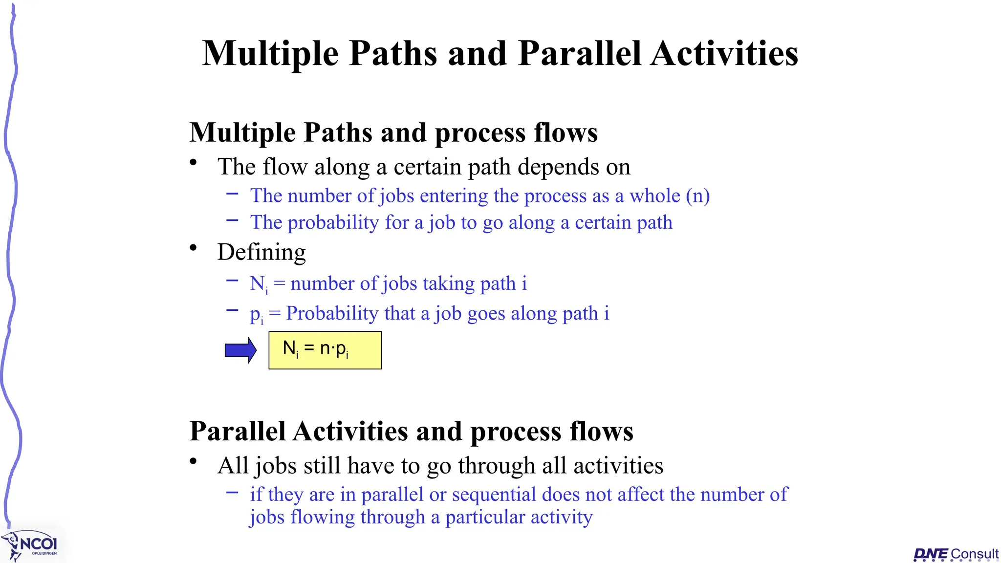
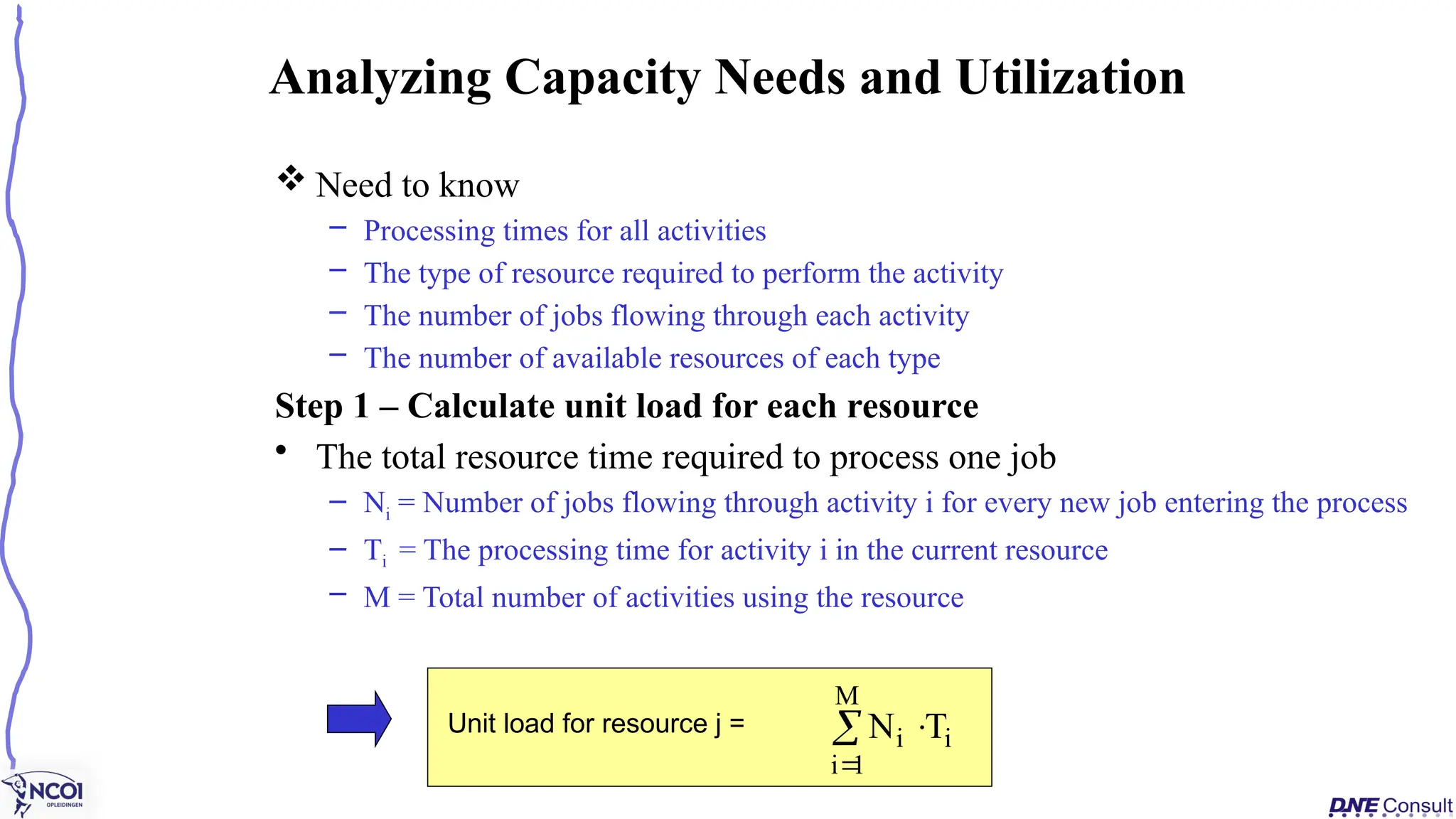

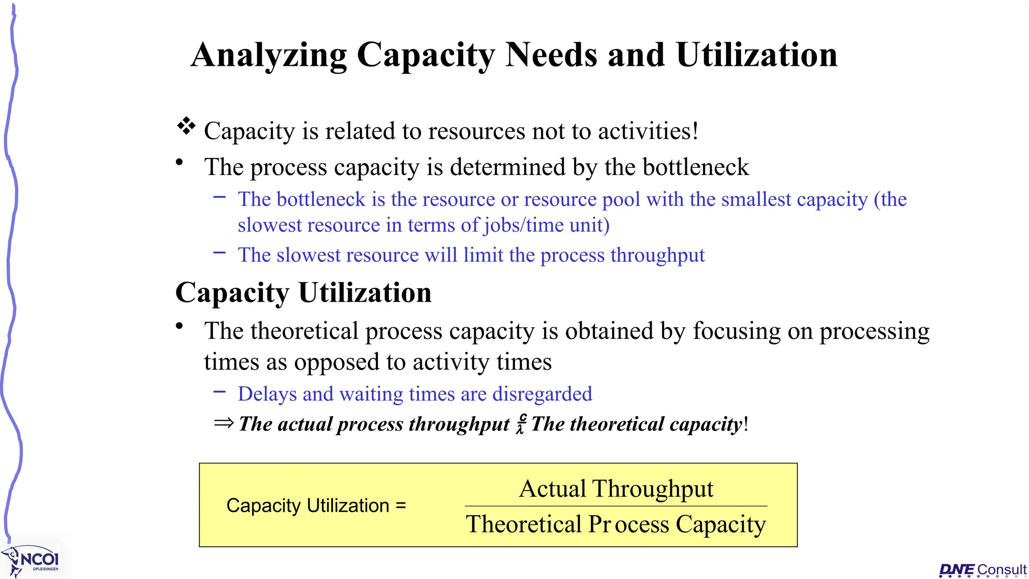
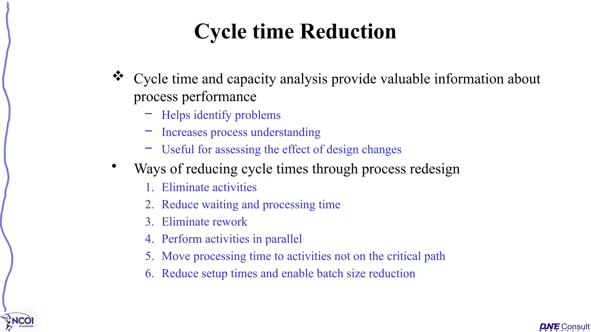
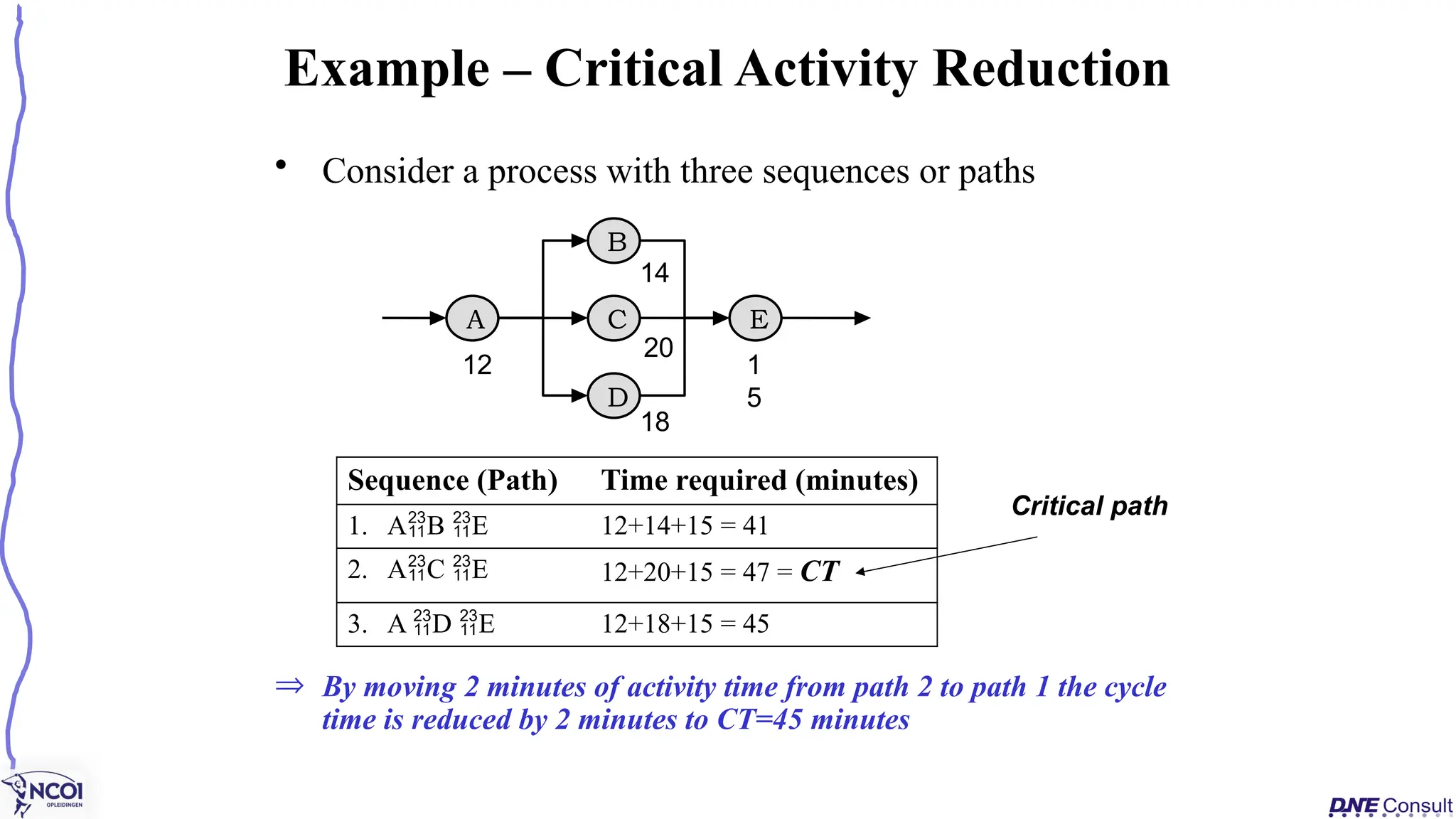
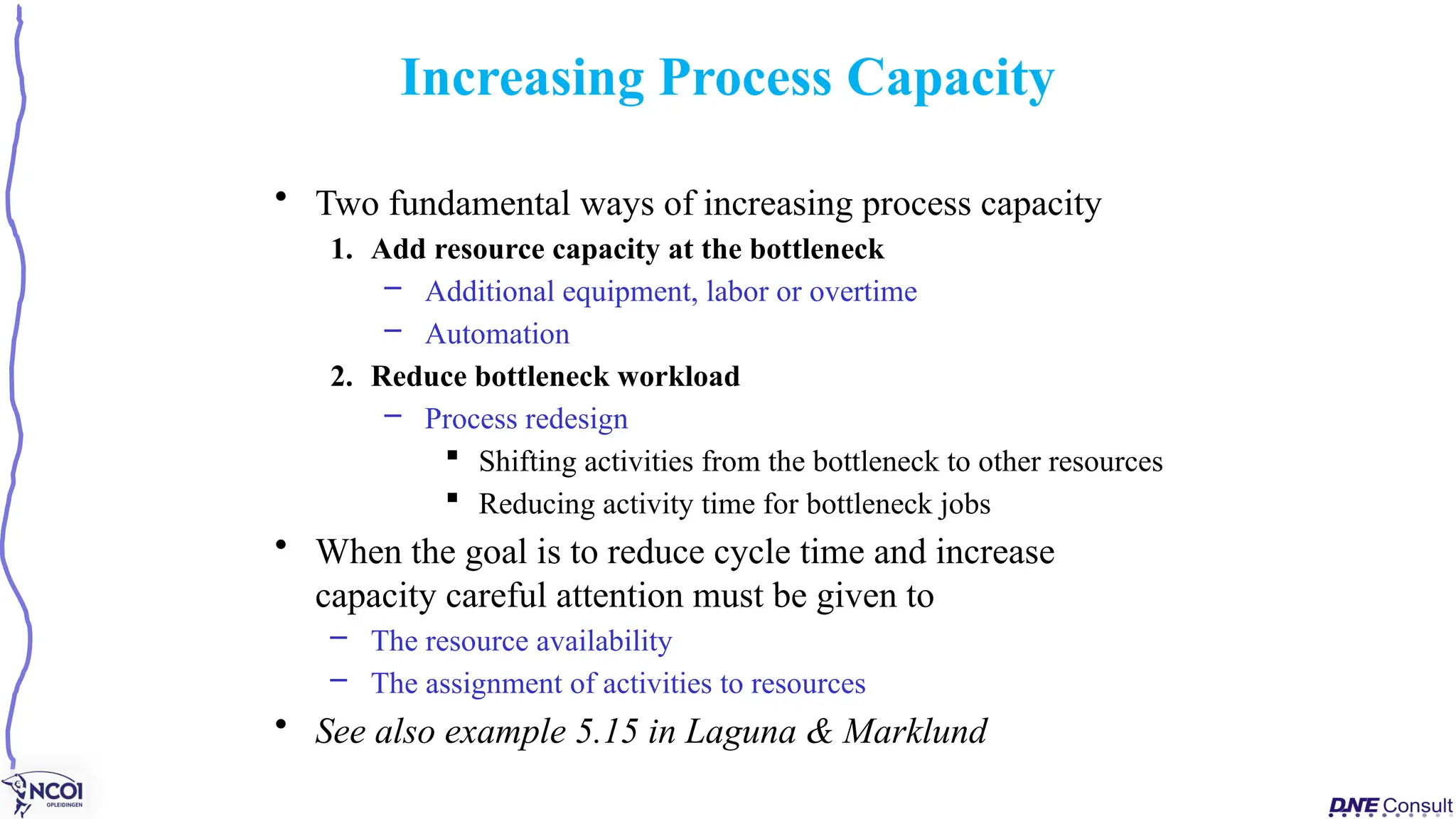
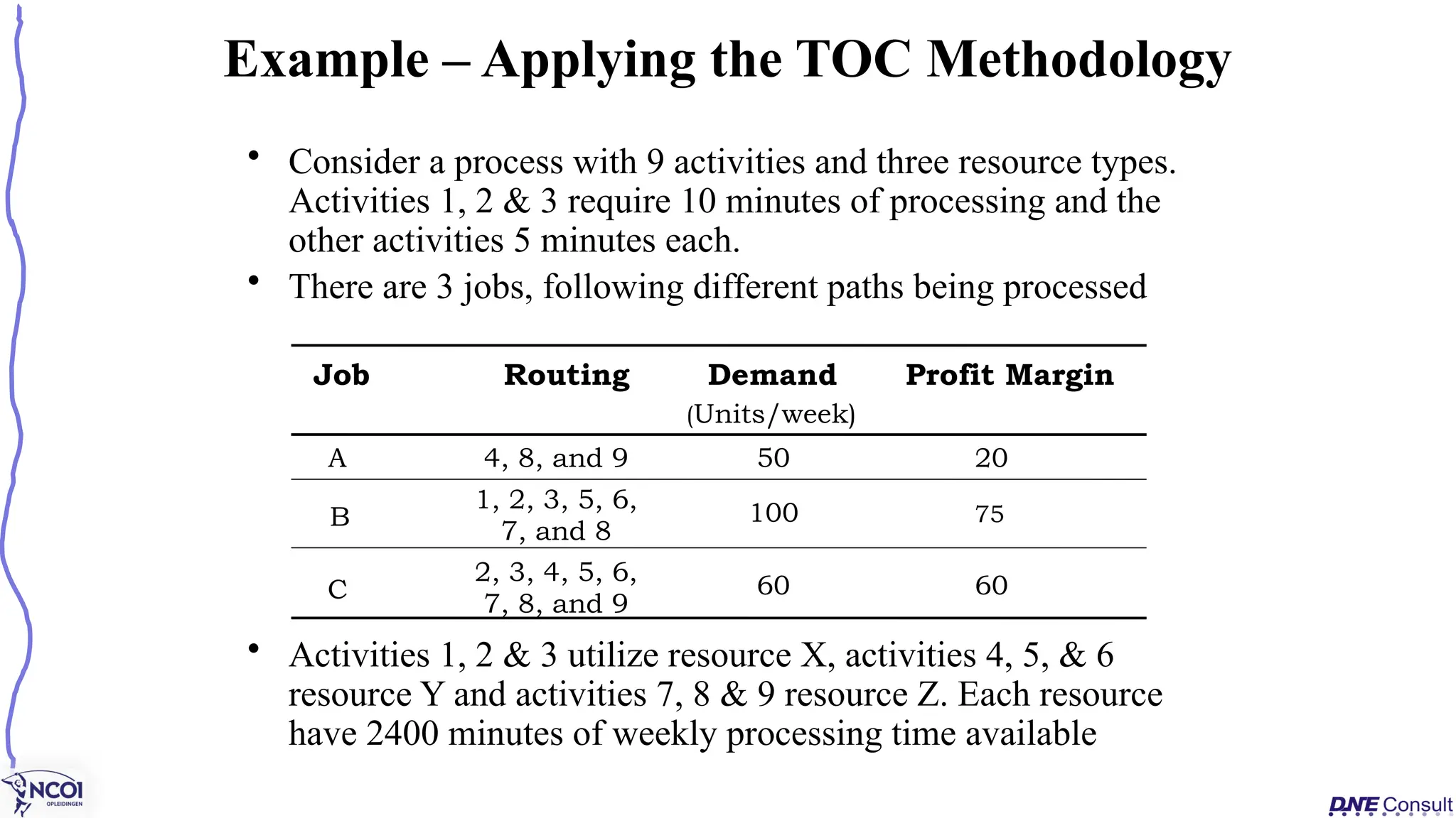
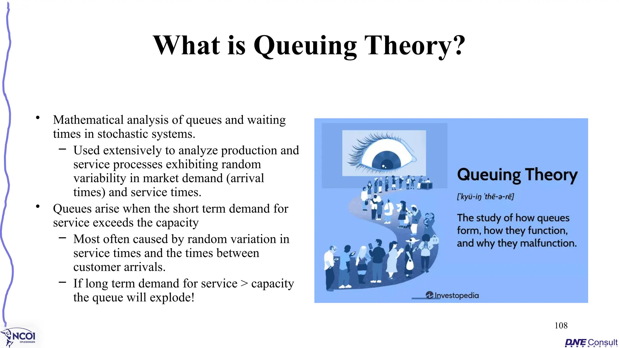
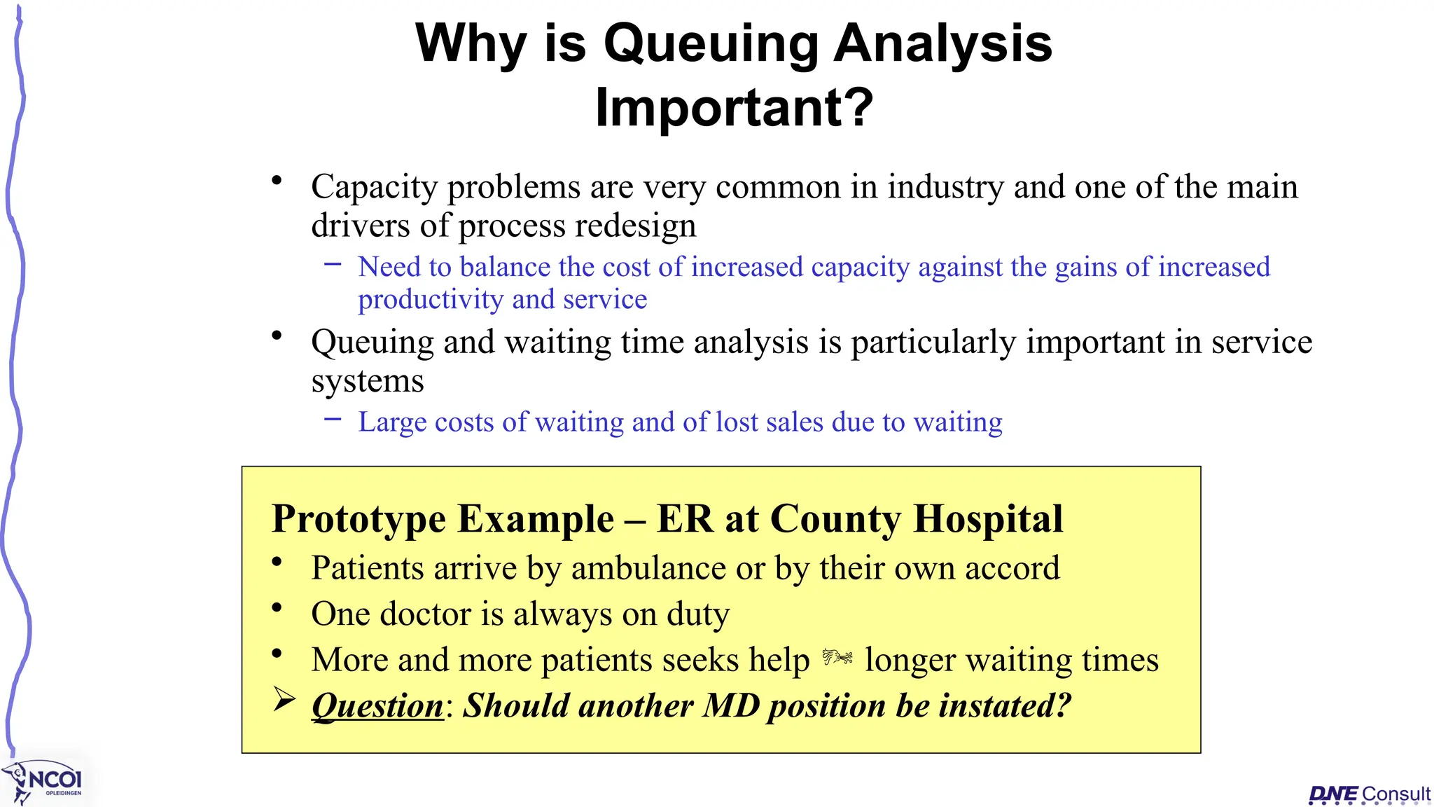
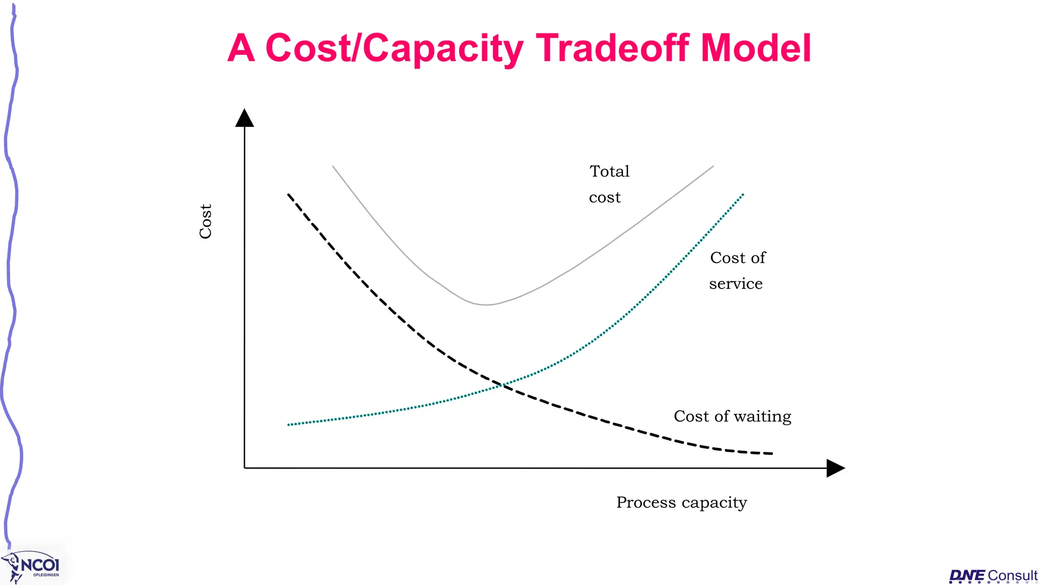

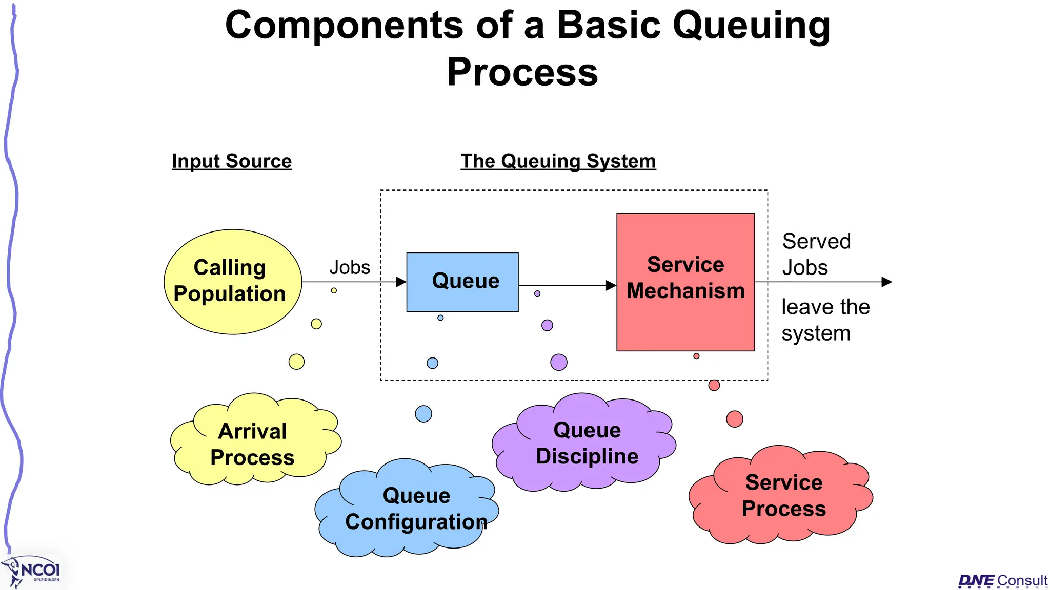
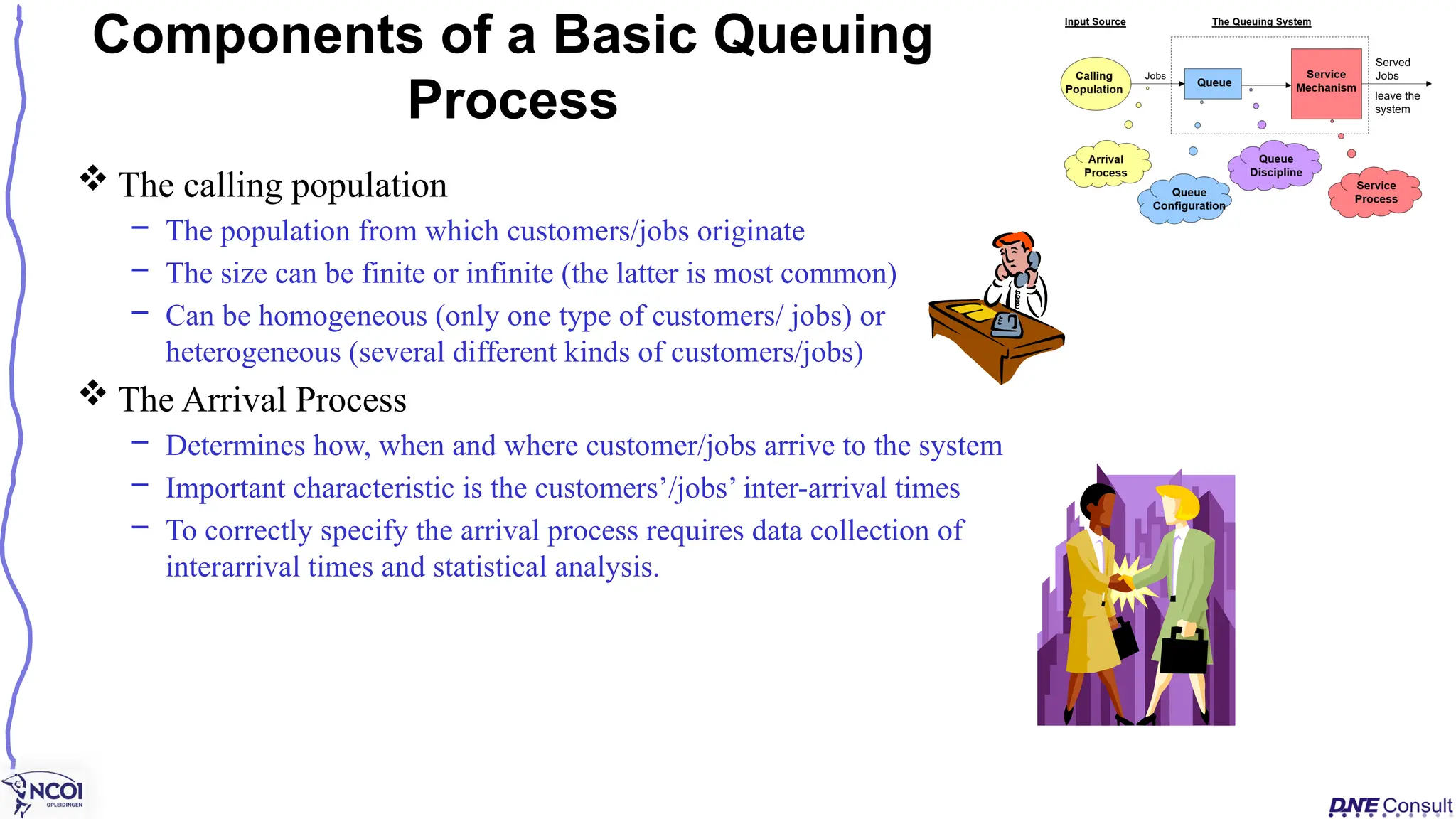

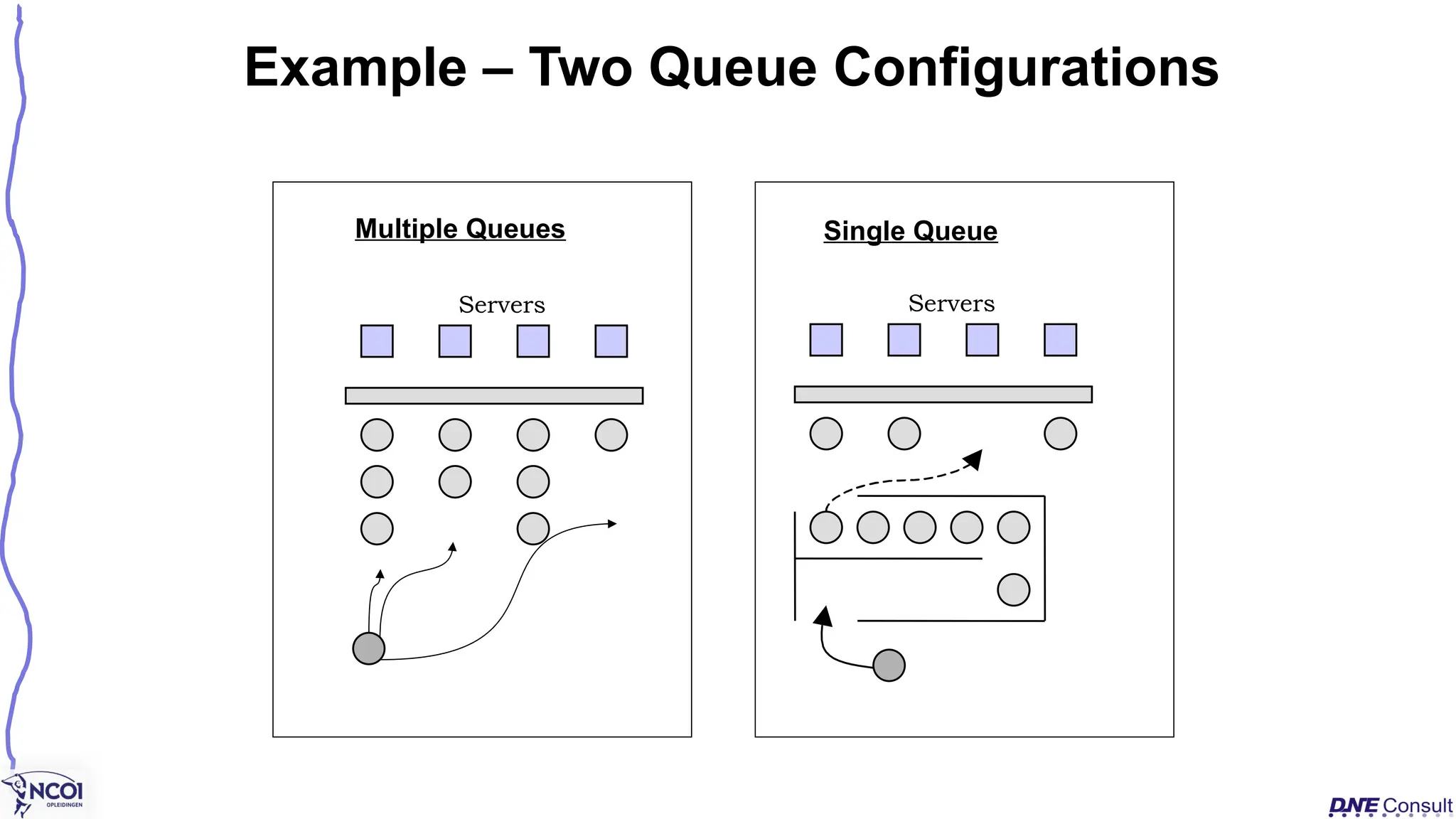
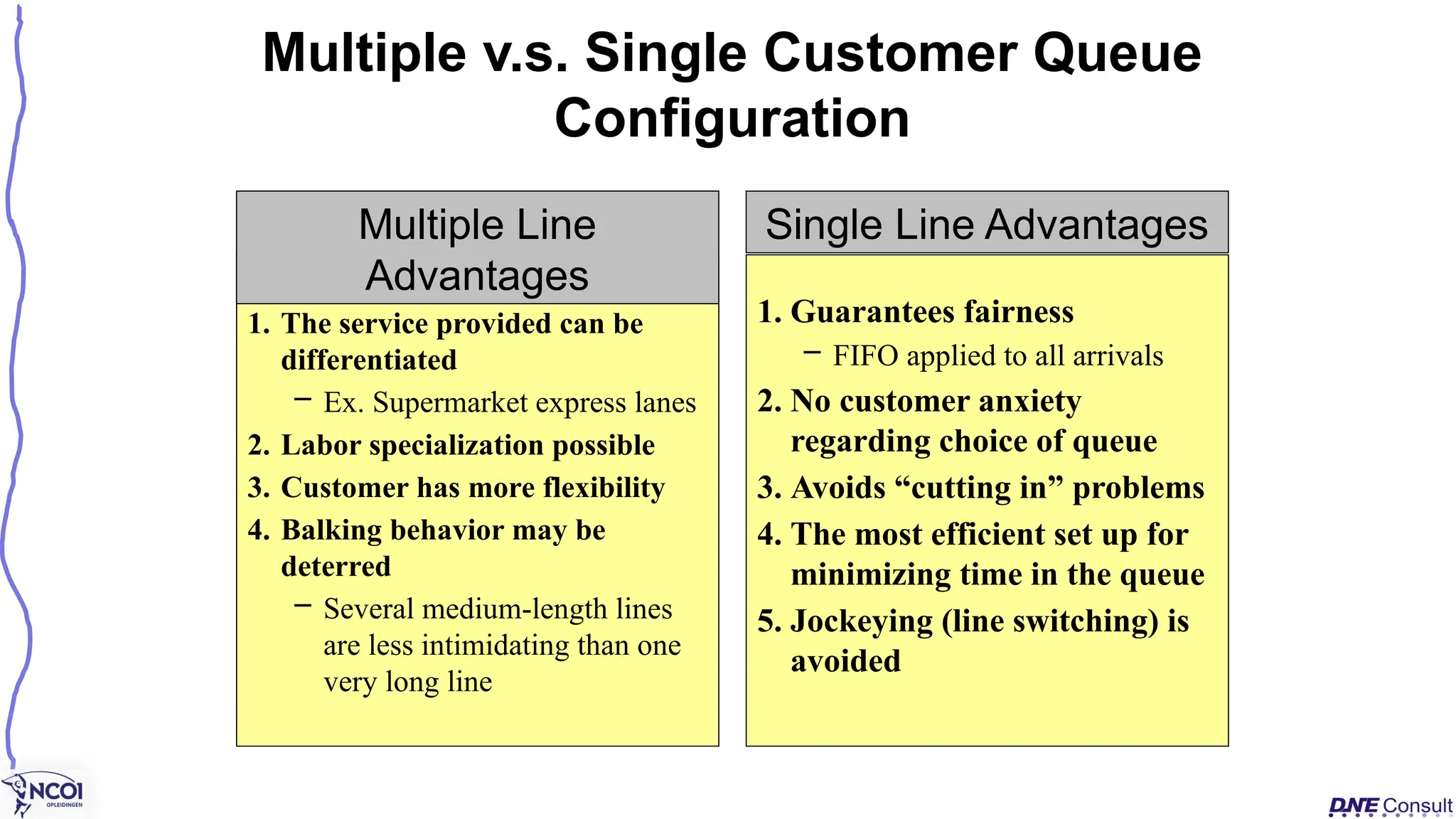
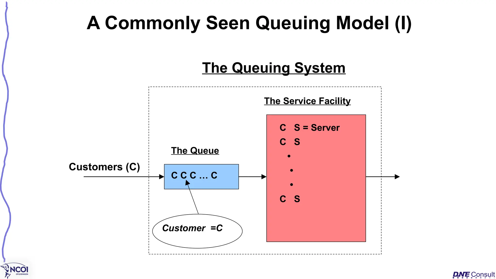
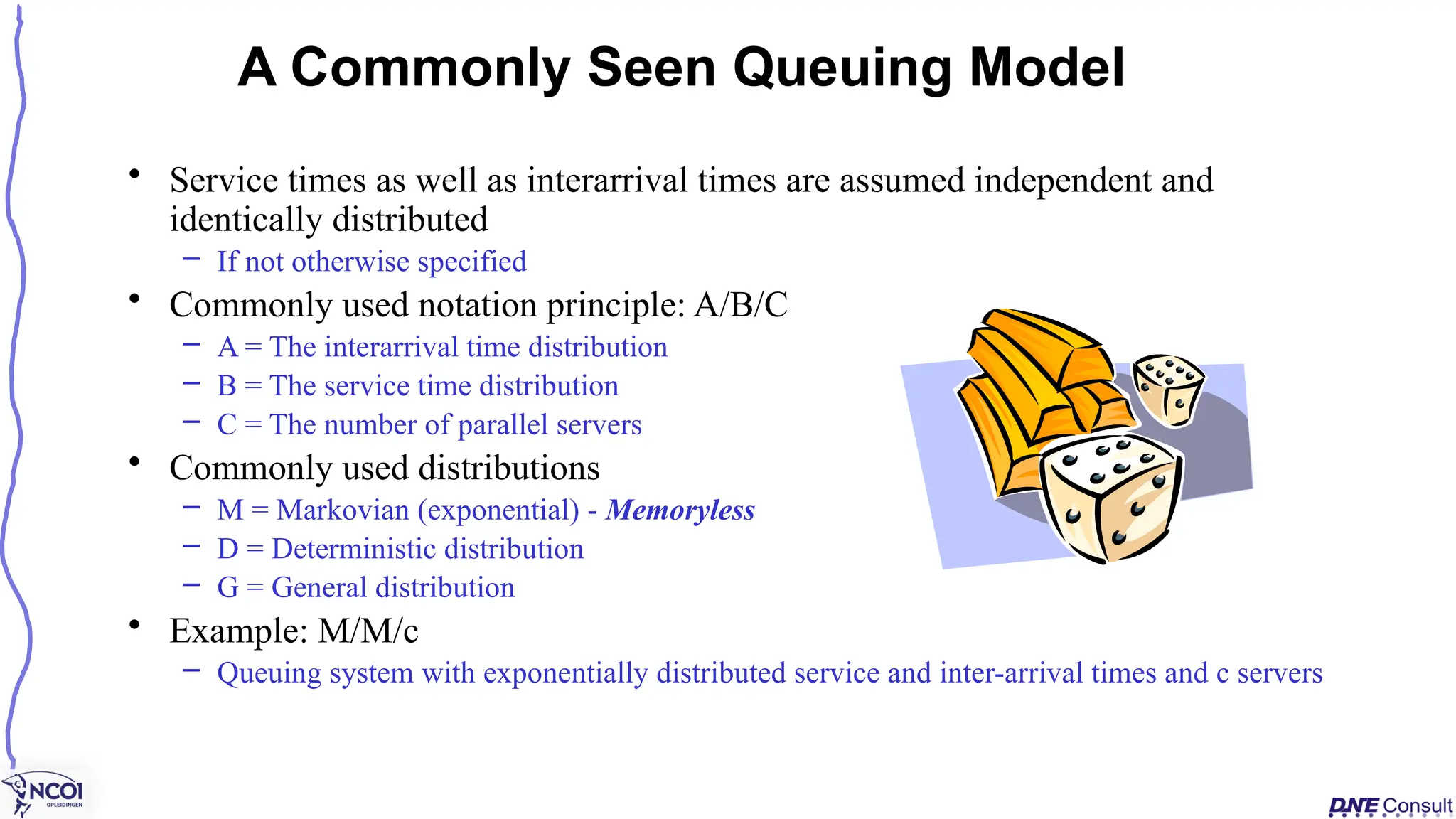
![The most commonly used queuing models are based on the
assumption of exponentially distributed service times and
interarrival times.
Definition: A stochastic (or random) variable Texp( ),
i.e., is exponentially distributed with parameter , if its
frequency function is:
The Exponential Distribution and
Queuing
0
t
when
0
0
t
when
e
)
t
(
f
t
T
t
T e
1
)
t
(
F
The Cumulative Distribution Function is:
The mean = E[T] = 1/
The Variance = Var[T] = 1/ 2
Stochastisch = De aanwezigheid
van een toevalsvariabele.
Een stochastisch proces houdt in dat
het systeem een element van toeval
kent (bijvoorbeeld merkenwissel
wordt vaak als
een stochastisch proces gezien).
T = random variabele representing
either interarrival times or services
times in a queuing proces.](https://image.slidesharecdn.com/mcbpm3-250413093009-970d90f4/75/Business-Process-Modeling-Theory-and-practice-119-2048.jpg)
![The Exponential Distribution
Time between arrivals
Mean=
E[T]=1/
Probability
density
t
fT(t)
](https://image.slidesharecdn.com/mcbpm3-250413093009-970d90f4/75/Business-Process-Modeling-Theory-and-practice-120-2048.jpg)
![ Relationship to the Poisson distribution and the Poisson Process
Let X(t) be the number of events occurring in the interval
[0,t]. If the time between consecutive events is T and
Texp()
X(t)Po(t) {X(t), t0} constitutes a Poisson Process
Properties of the Exp-distribution (IV)
...
,
1
,
0
n
for
!
n
e
)
t
(
)
n
)
t
(
X
(
P
nt
n
](https://image.slidesharecdn.com/mcbpm3-250413093009-970d90f4/75/Business-Process-Modeling-Theory-and-practice-121-2048.jpg)
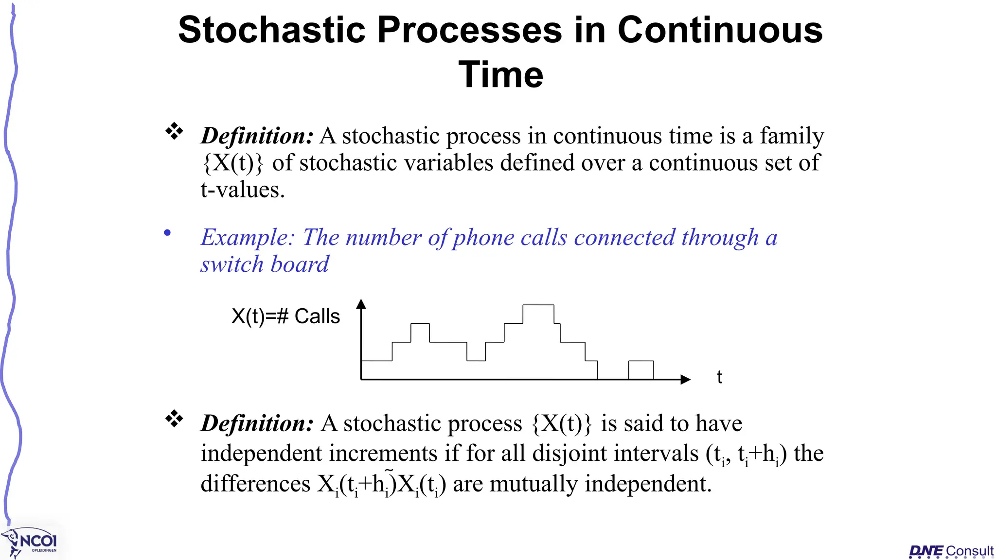
![ The standard assumption in many queuing models is that the
arrival process is Poisson
Two equivalent definitions of the Poisson Process
1. The times between arrivals are independent, identically
distributed and exponential
2. X(t) is a Poisson process with arrival rate iff.
a) X(t) have independent increments
b) For a small time interval h it holds that
P(exactly 1 event occurs in the interval [t, t+h]) = h + o(h)
P(more than 1 event occurs in the interval [t, t+h]) = o(h)
The Poisson Process](https://image.slidesharecdn.com/mcbpm3-250413093009-970d90f4/75/Business-Process-Modeling-Theory-and-practice-123-2048.jpg)
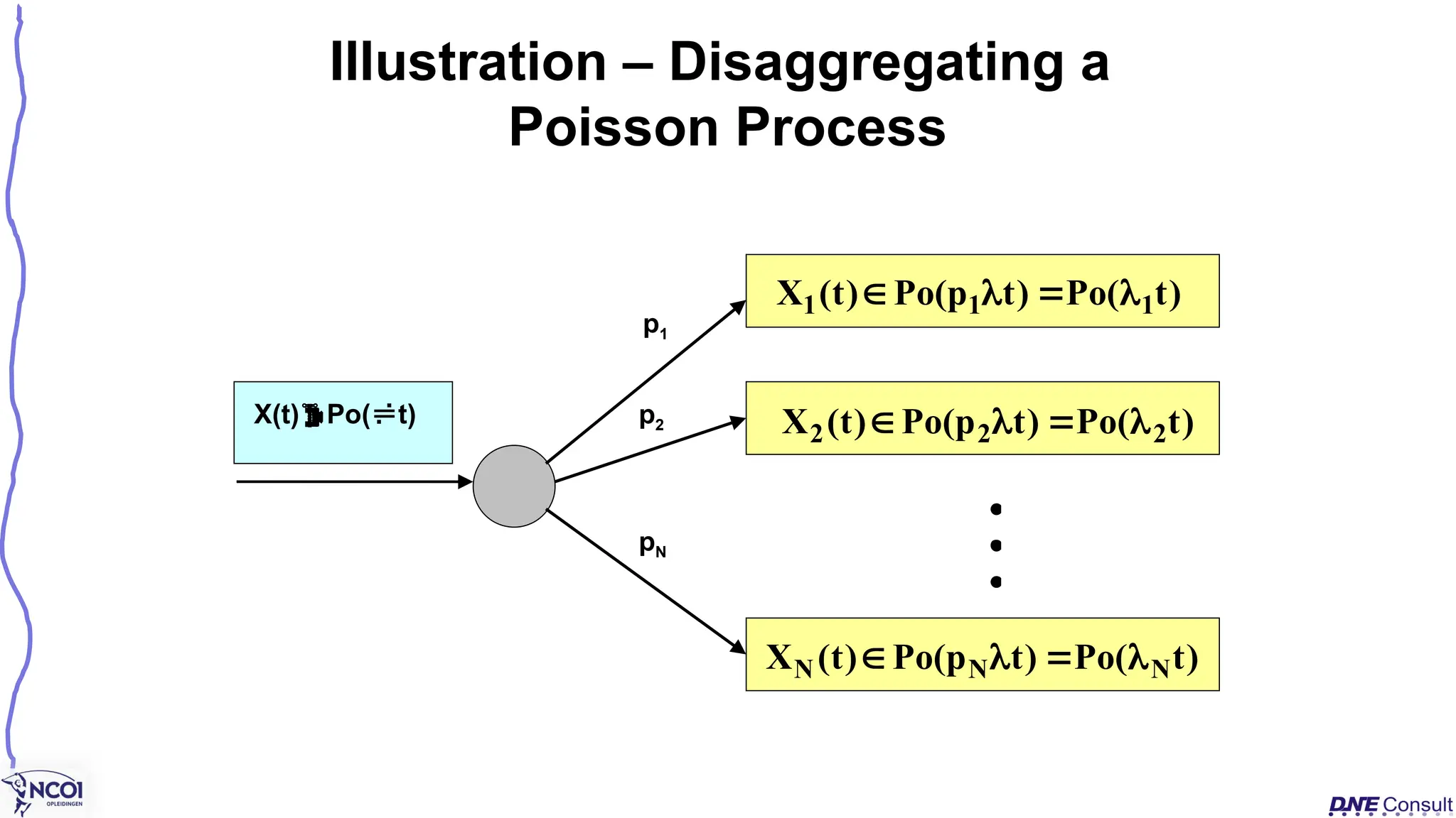
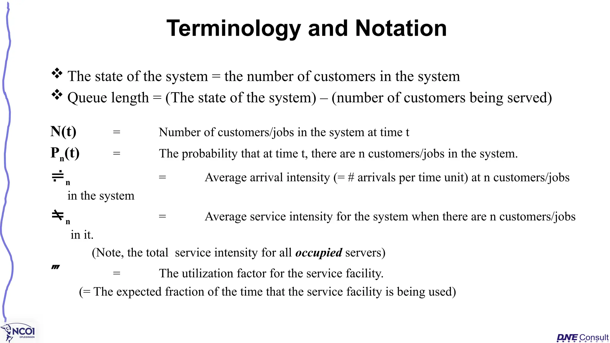
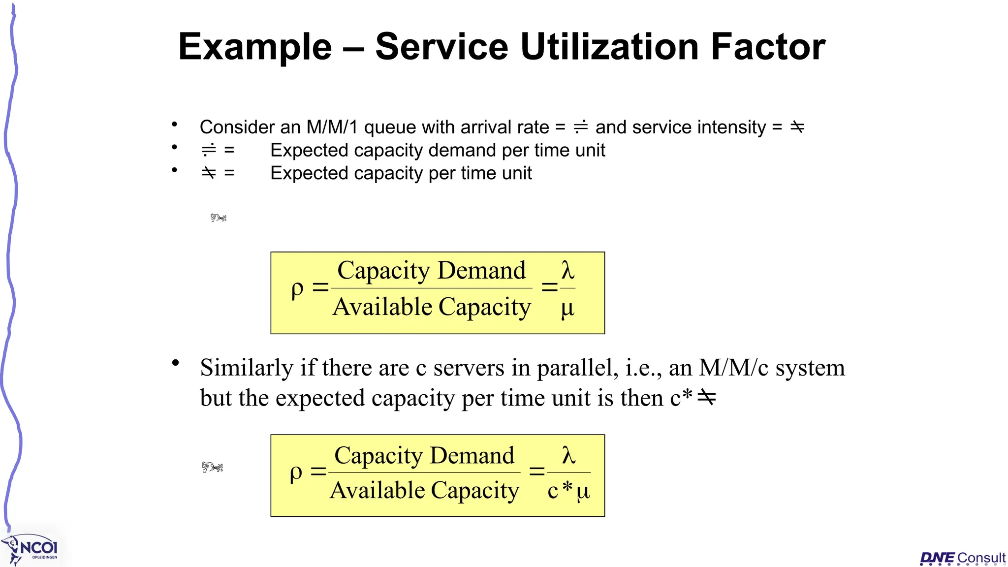

![Transient and Steady State Conditions
• Illustration of transient and steady-state conditions
– N(t) = number of customers in the system at time t,
– E[N(t)] = represents the expected number of customers in the system.
Transient condition
0
5
10
15
20
25
30
0 5 10 15 20 25 30 35 40 45 50
time, t
Number
of
jobs
in
the
system,
N(t)
Steady State condition
E[N(t)]
N(t)](https://image.slidesharecdn.com/mcbpm3-250413093009-970d90f4/75/Business-Process-Modeling-Theory-and-practice-128-2048.jpg)