Download as PDF, PPTX

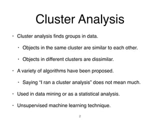
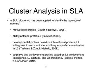

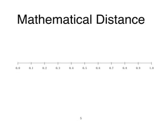
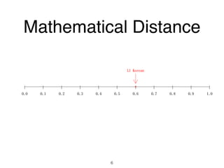
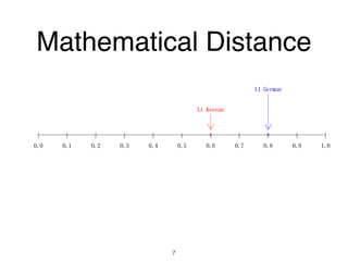

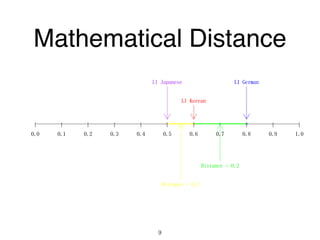
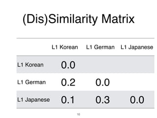

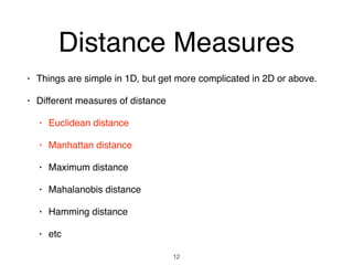

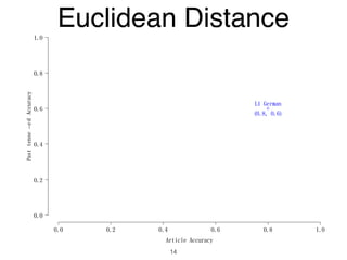
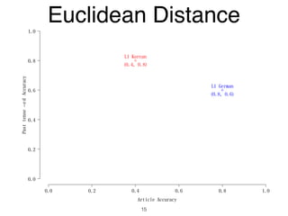
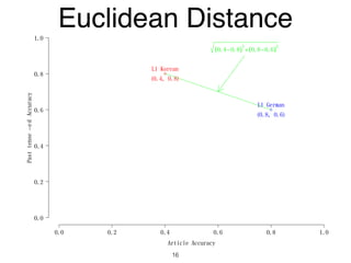
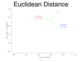
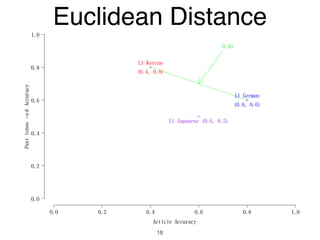
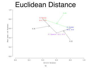
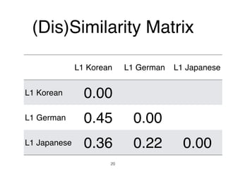
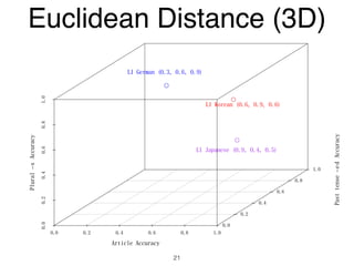
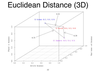

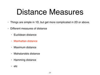
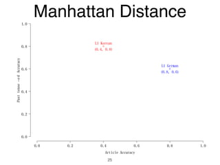
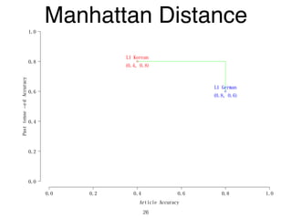
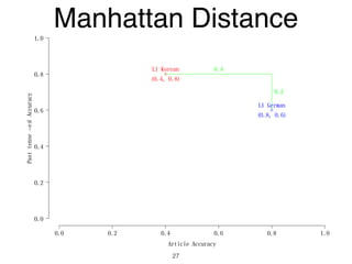
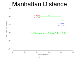
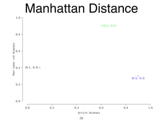
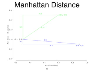
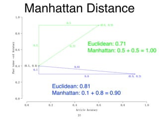
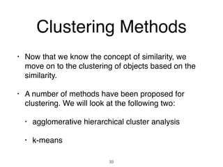
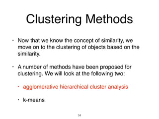


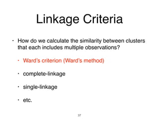

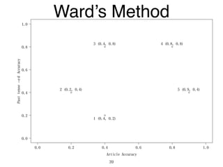
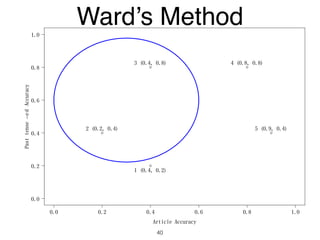

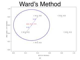
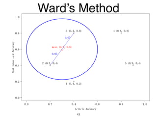
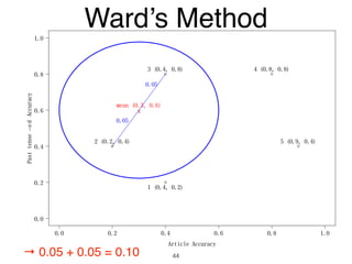
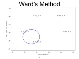
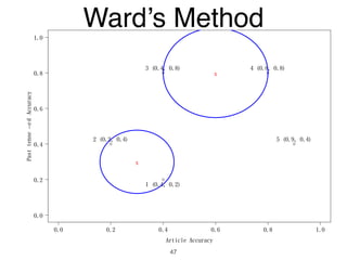
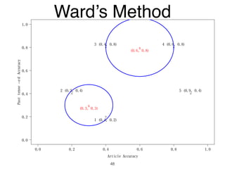
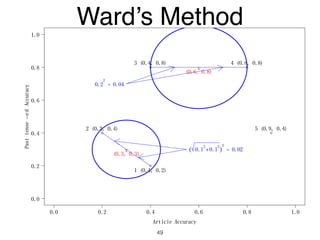
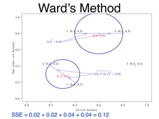
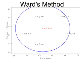

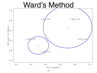
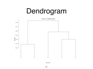


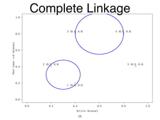
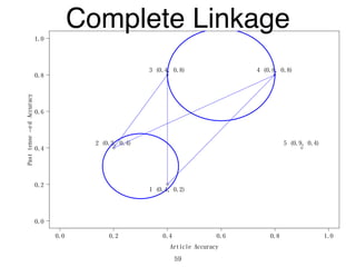
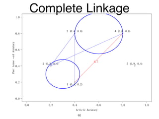
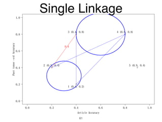

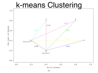
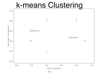
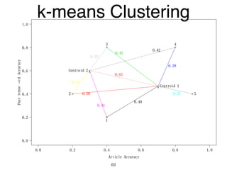
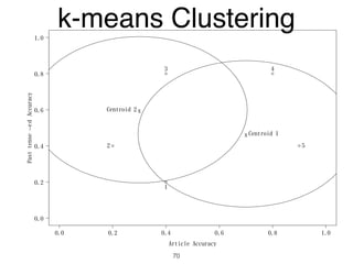
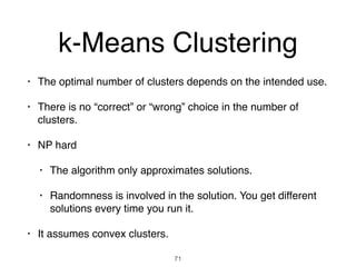


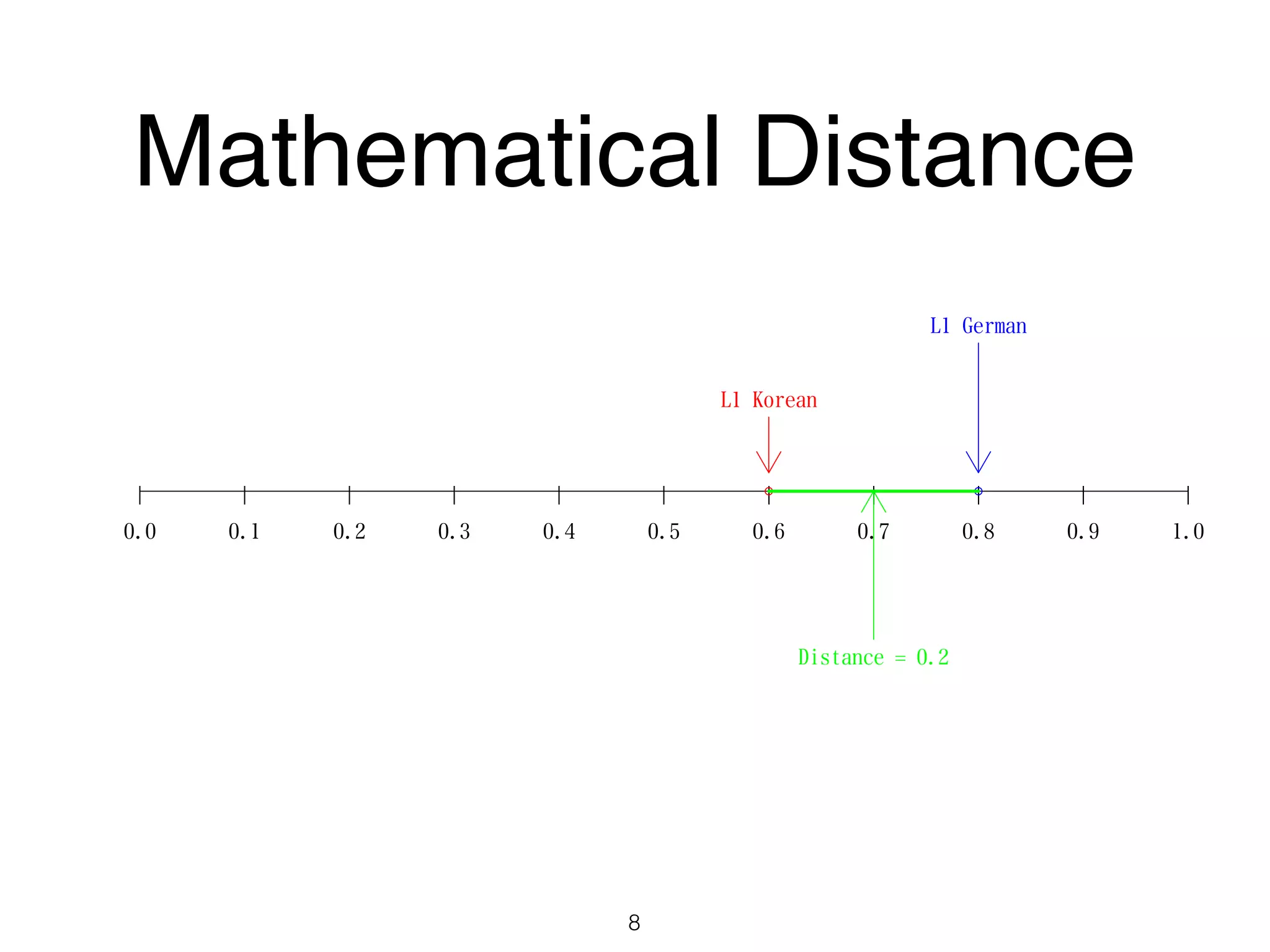
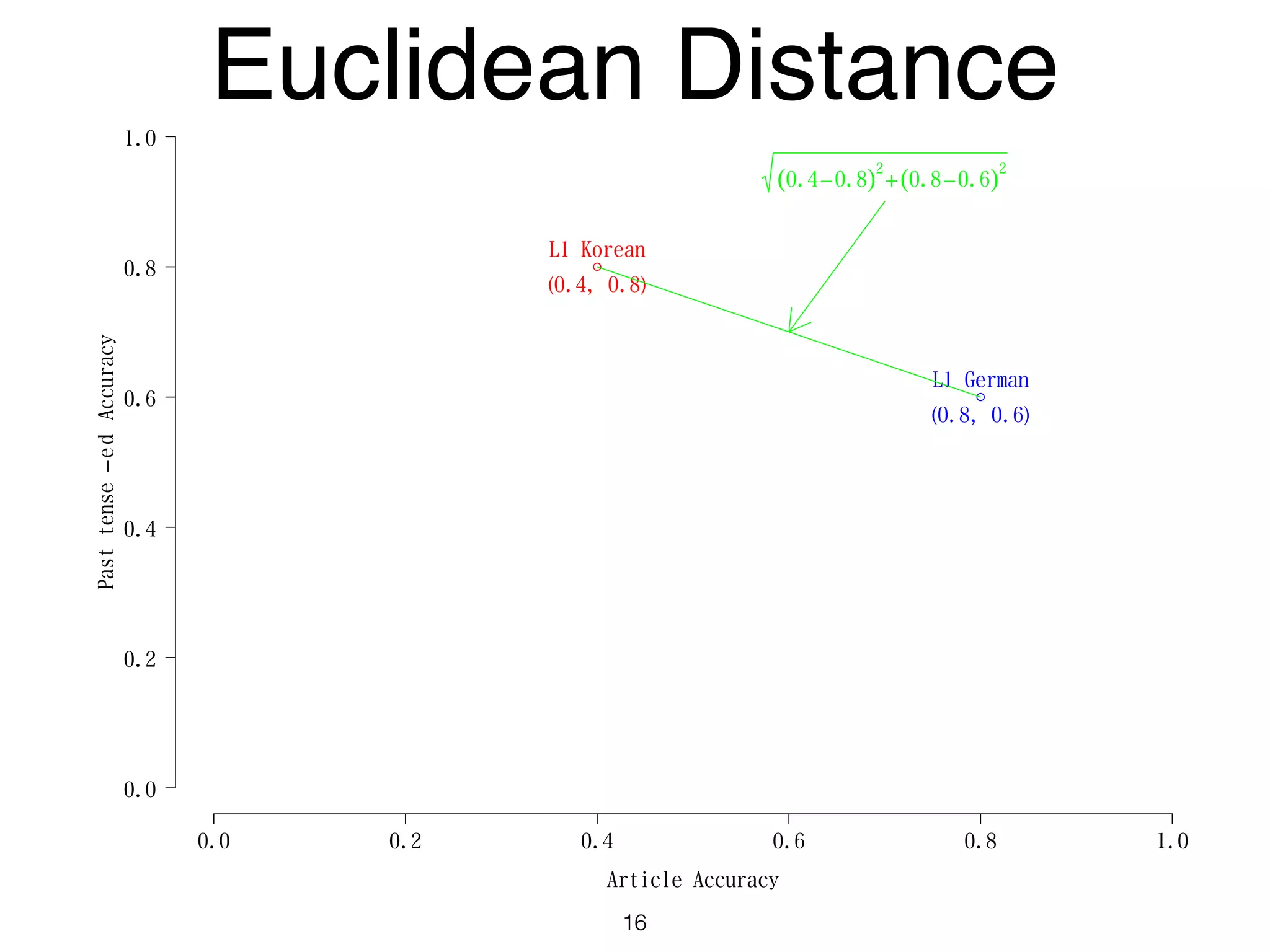
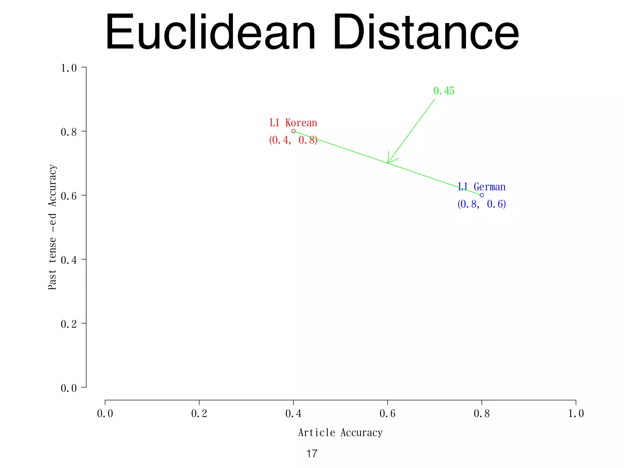
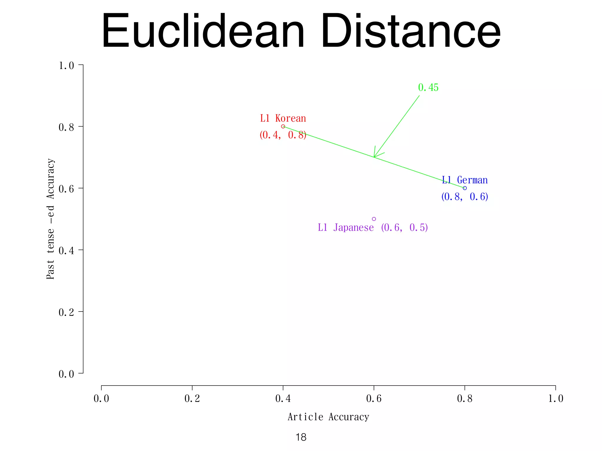
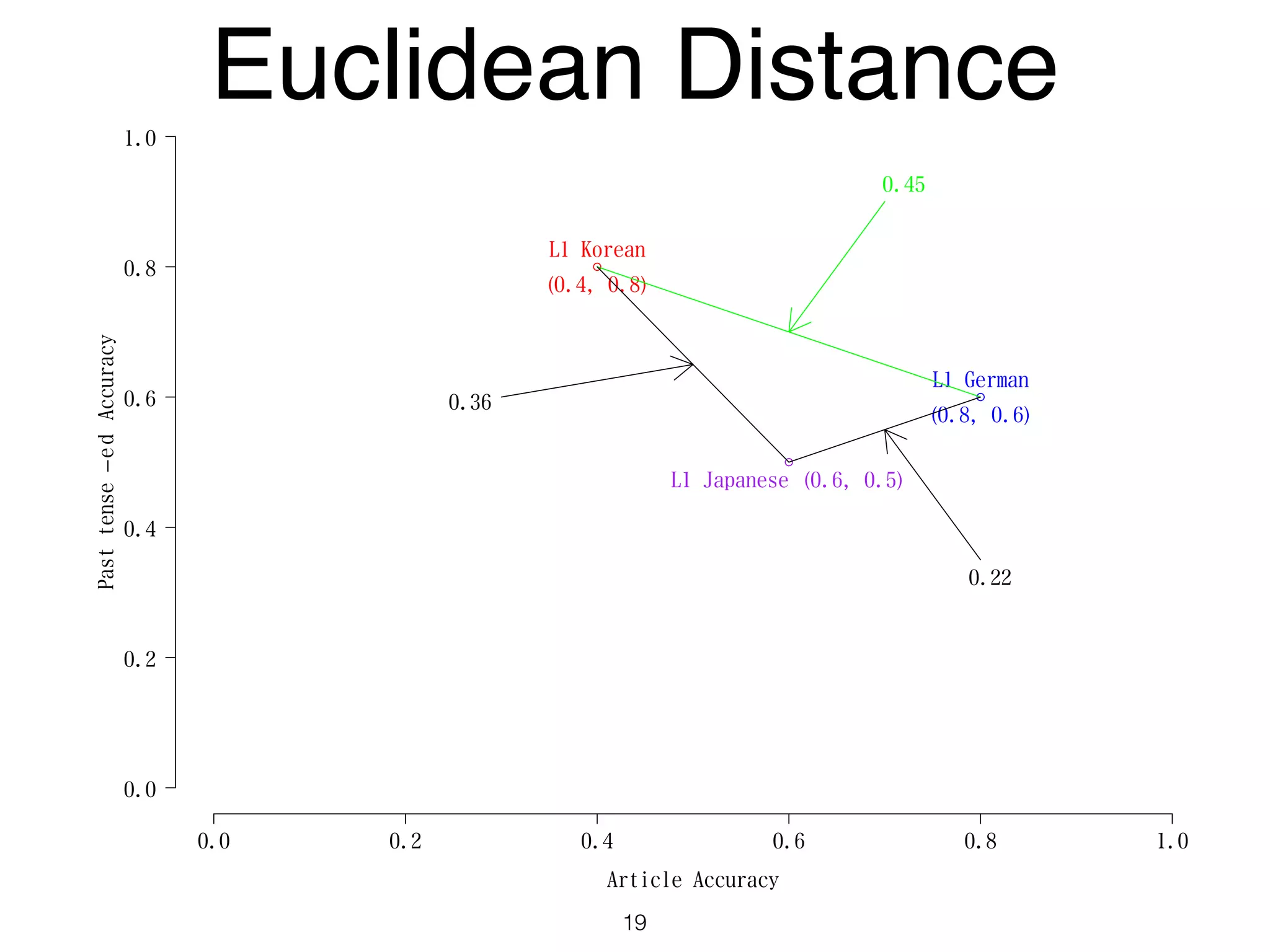
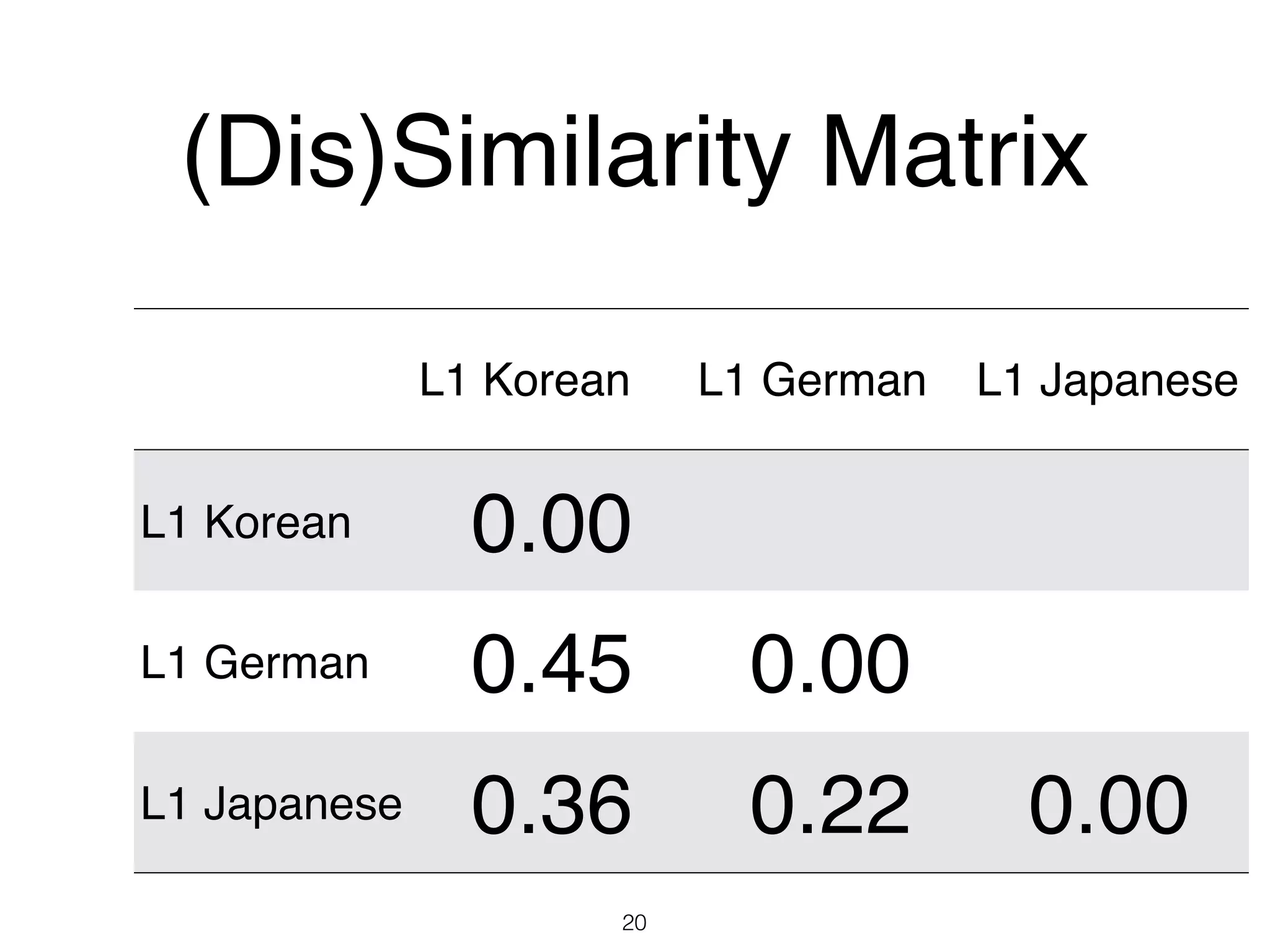
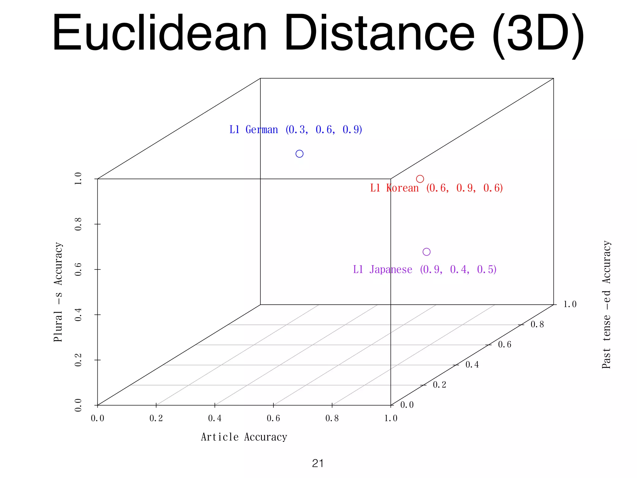
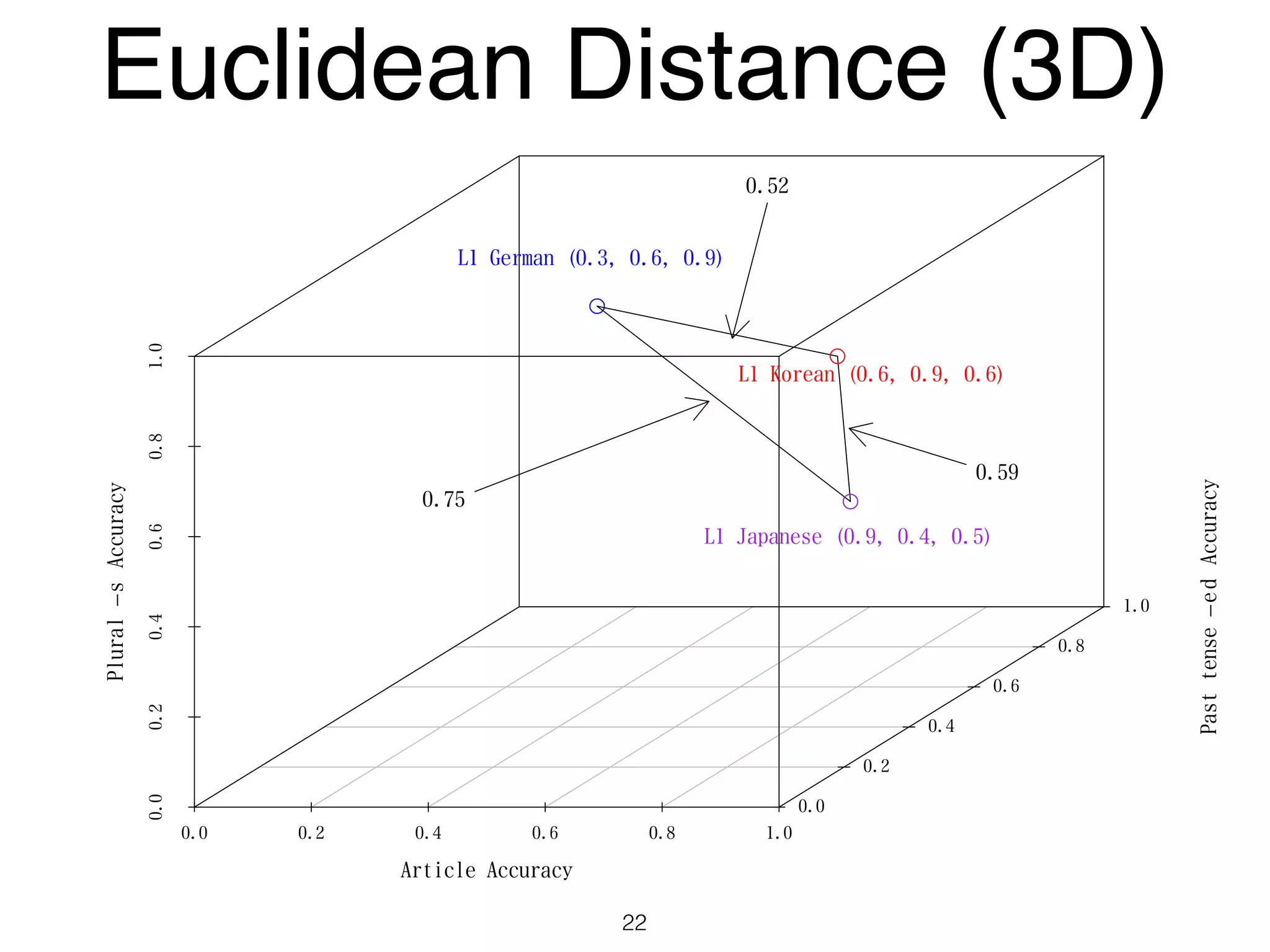
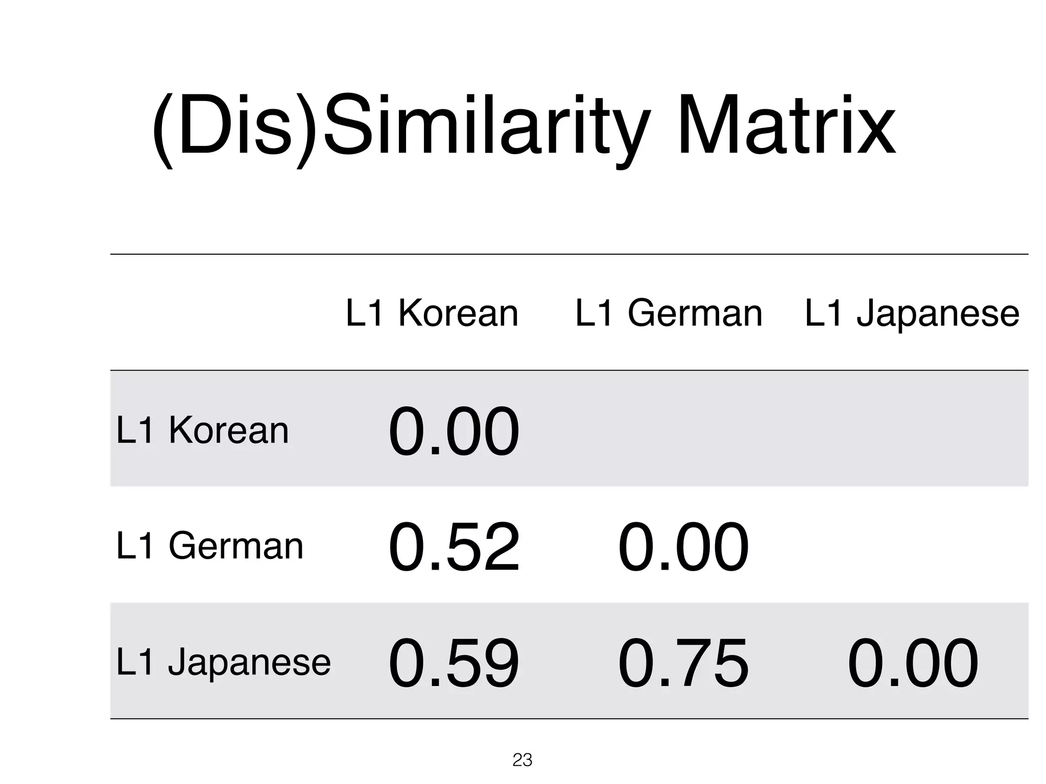
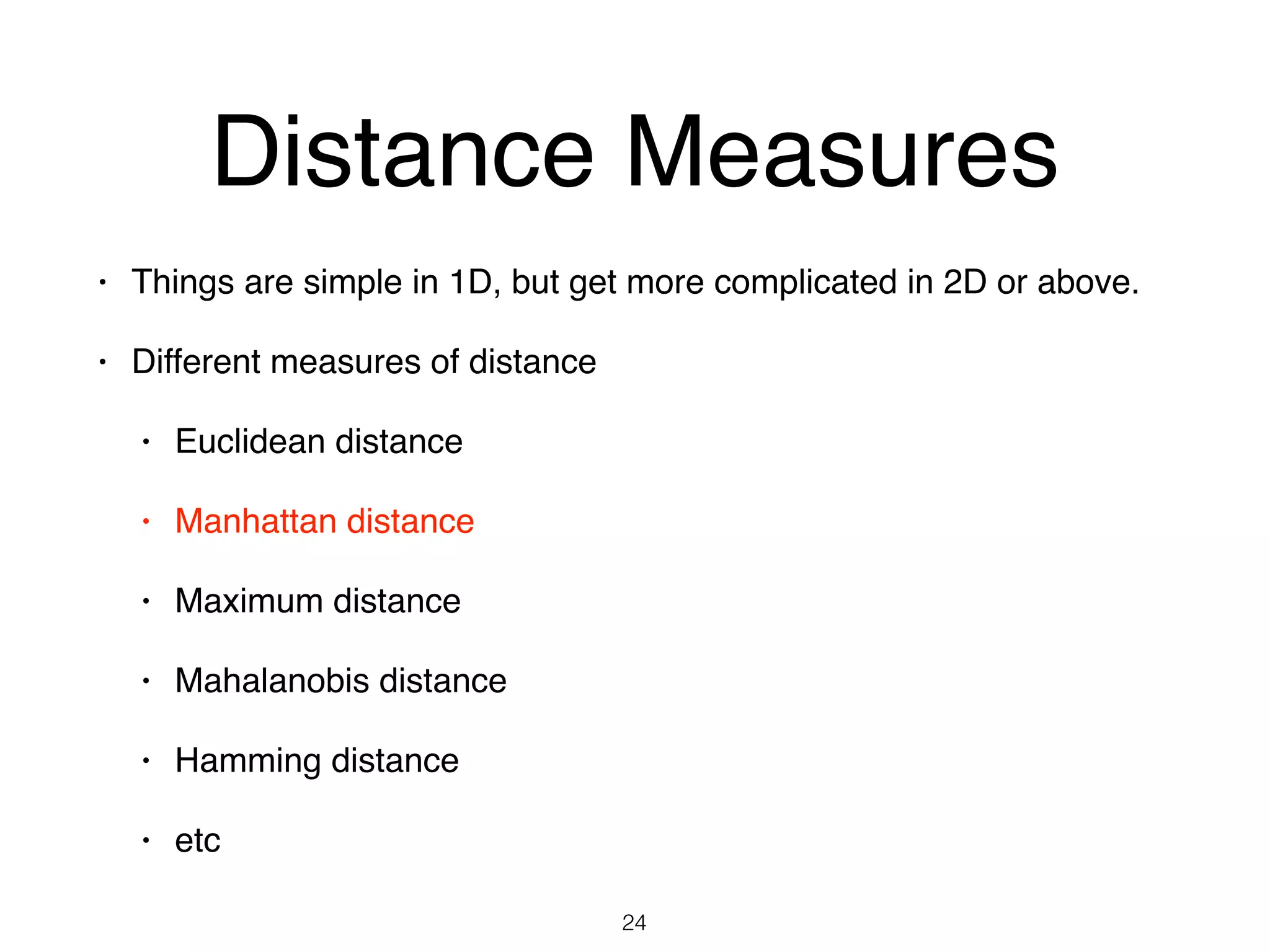
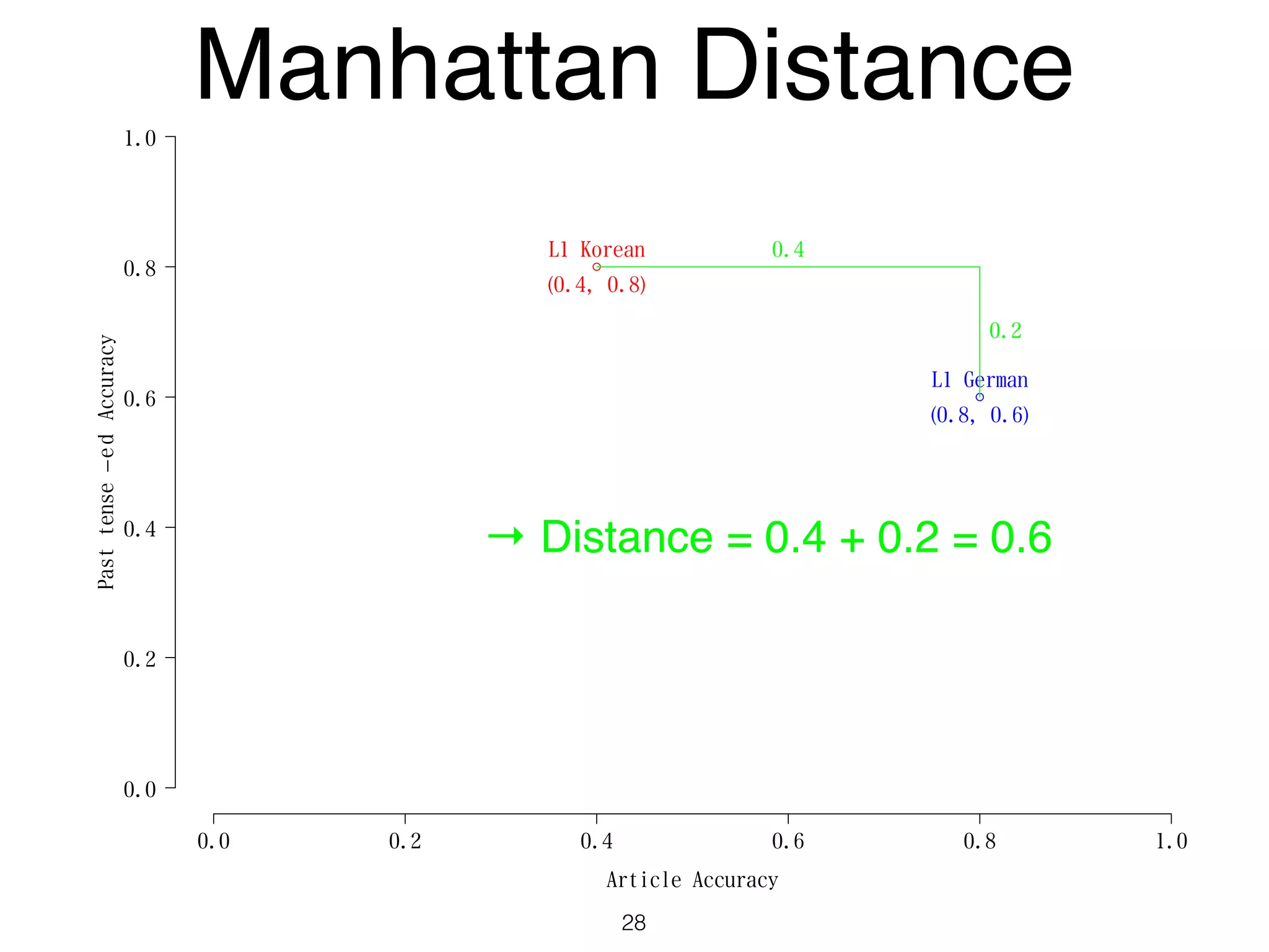


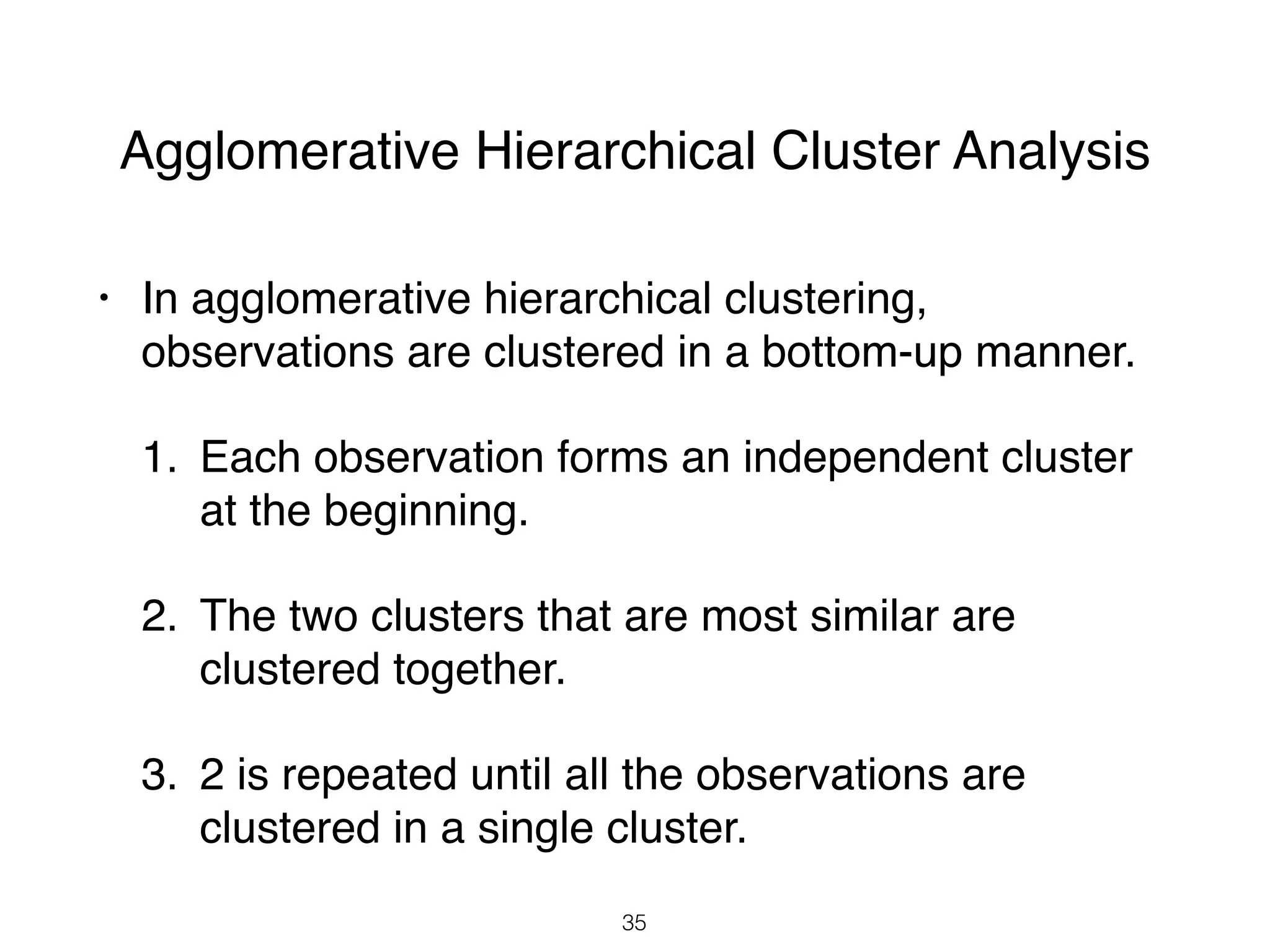
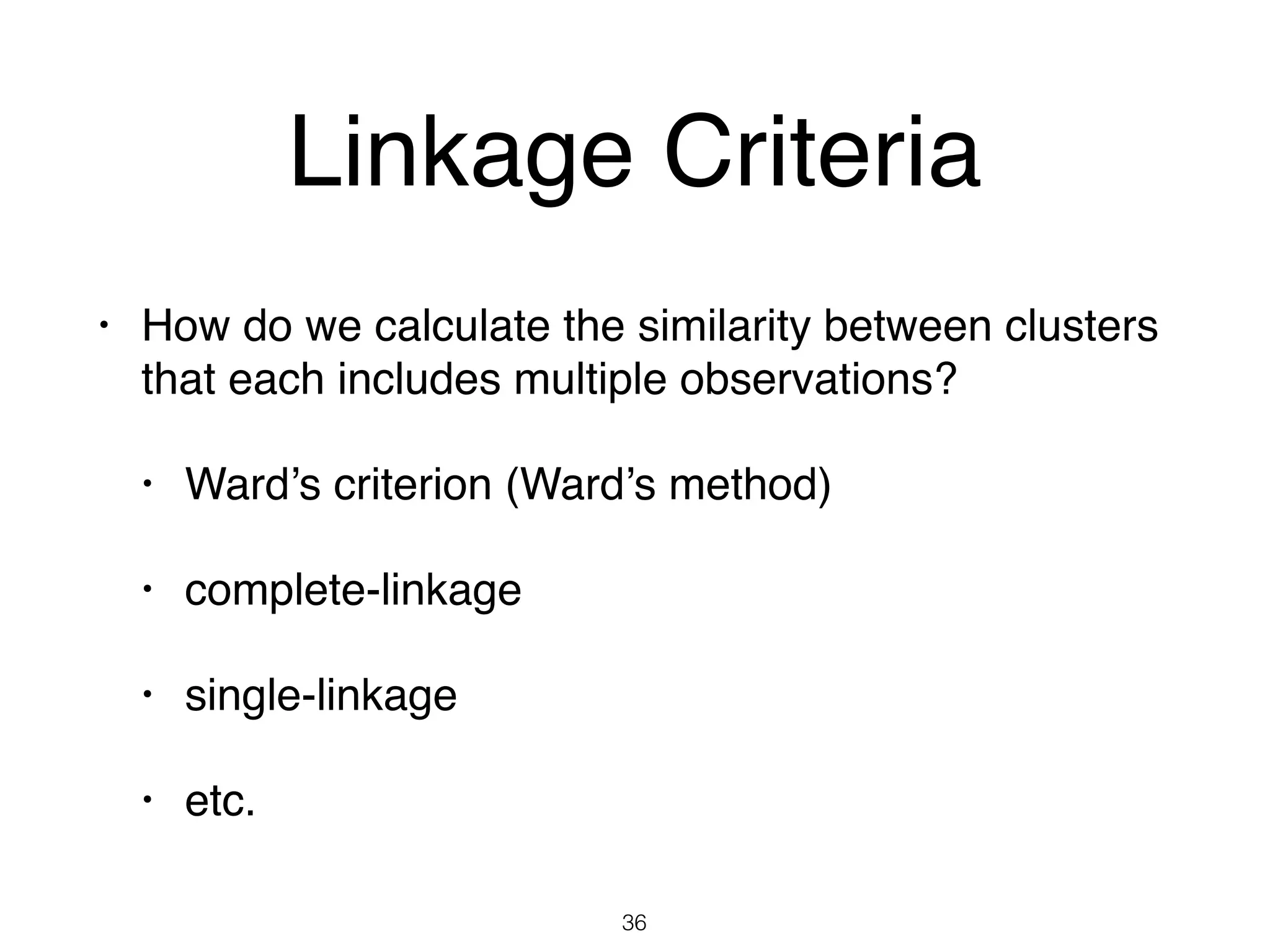
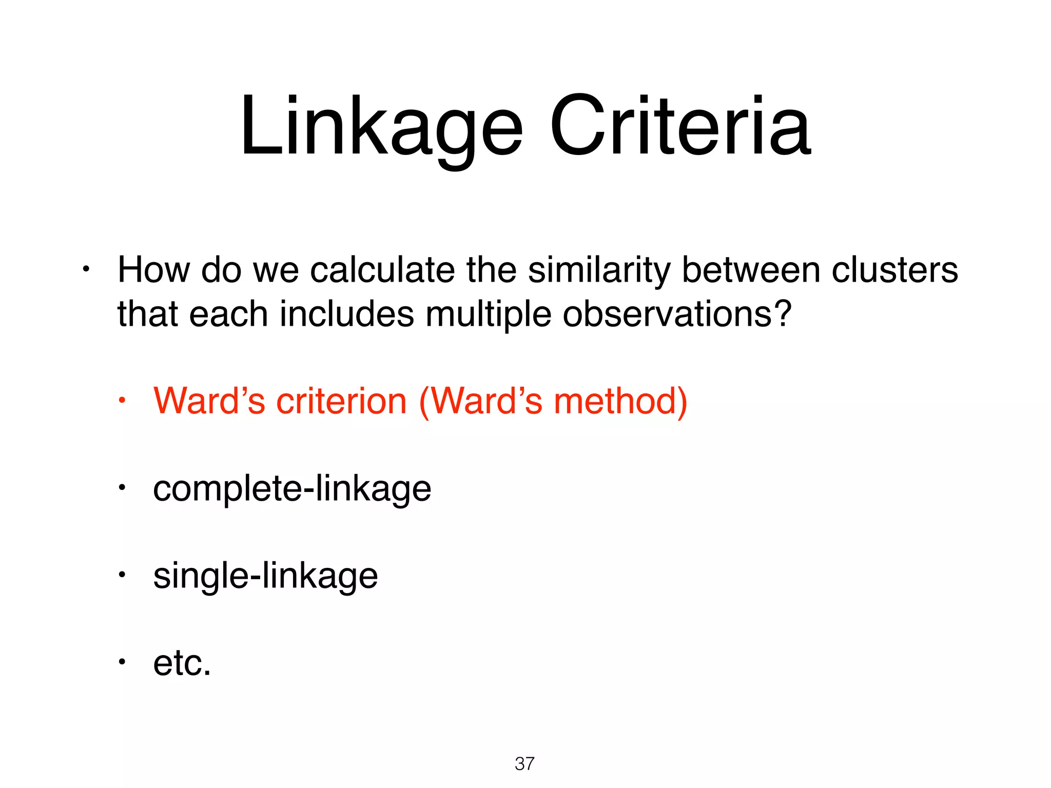
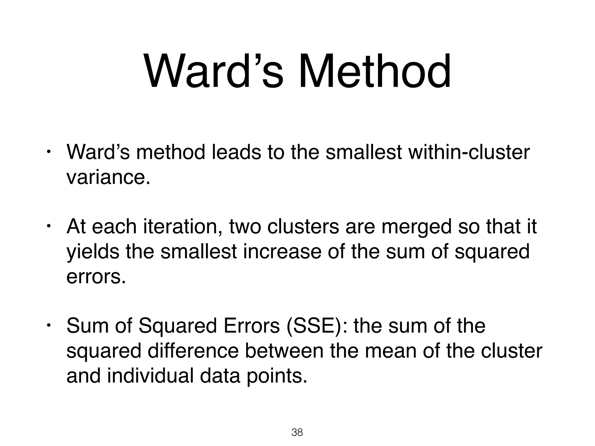
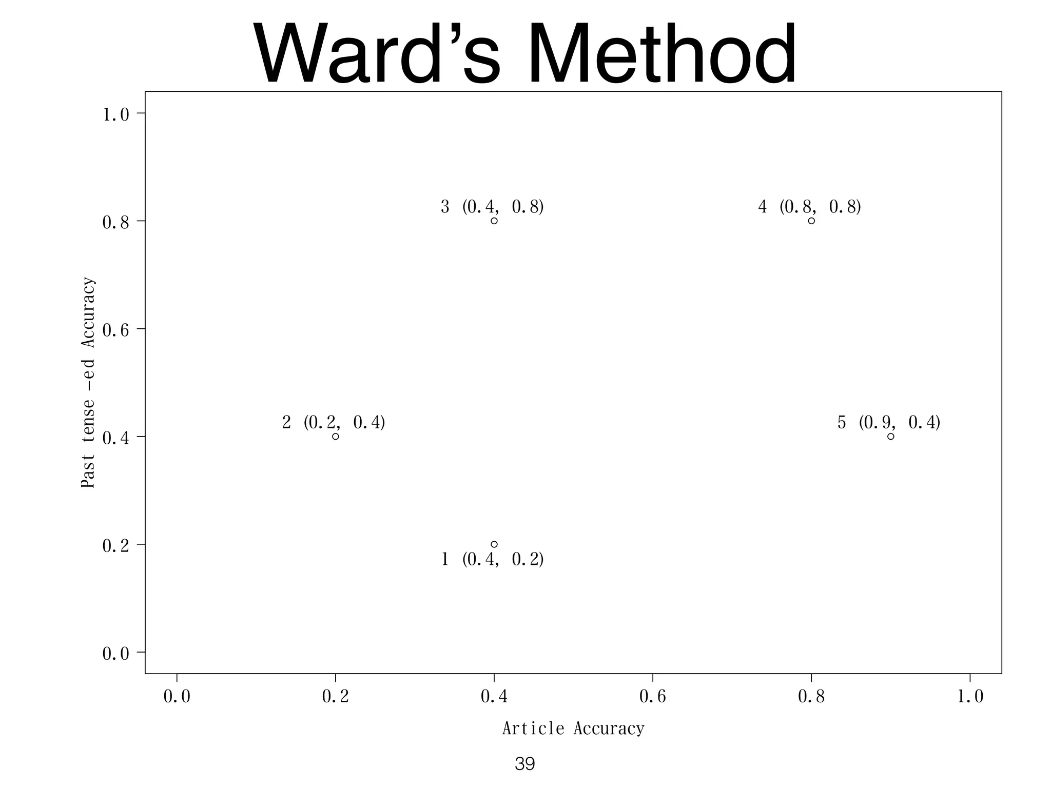
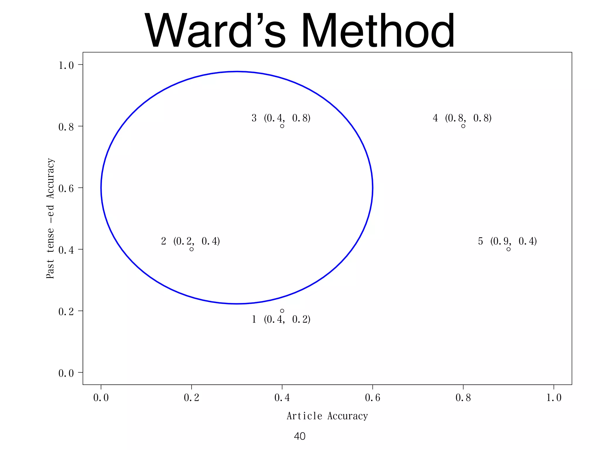
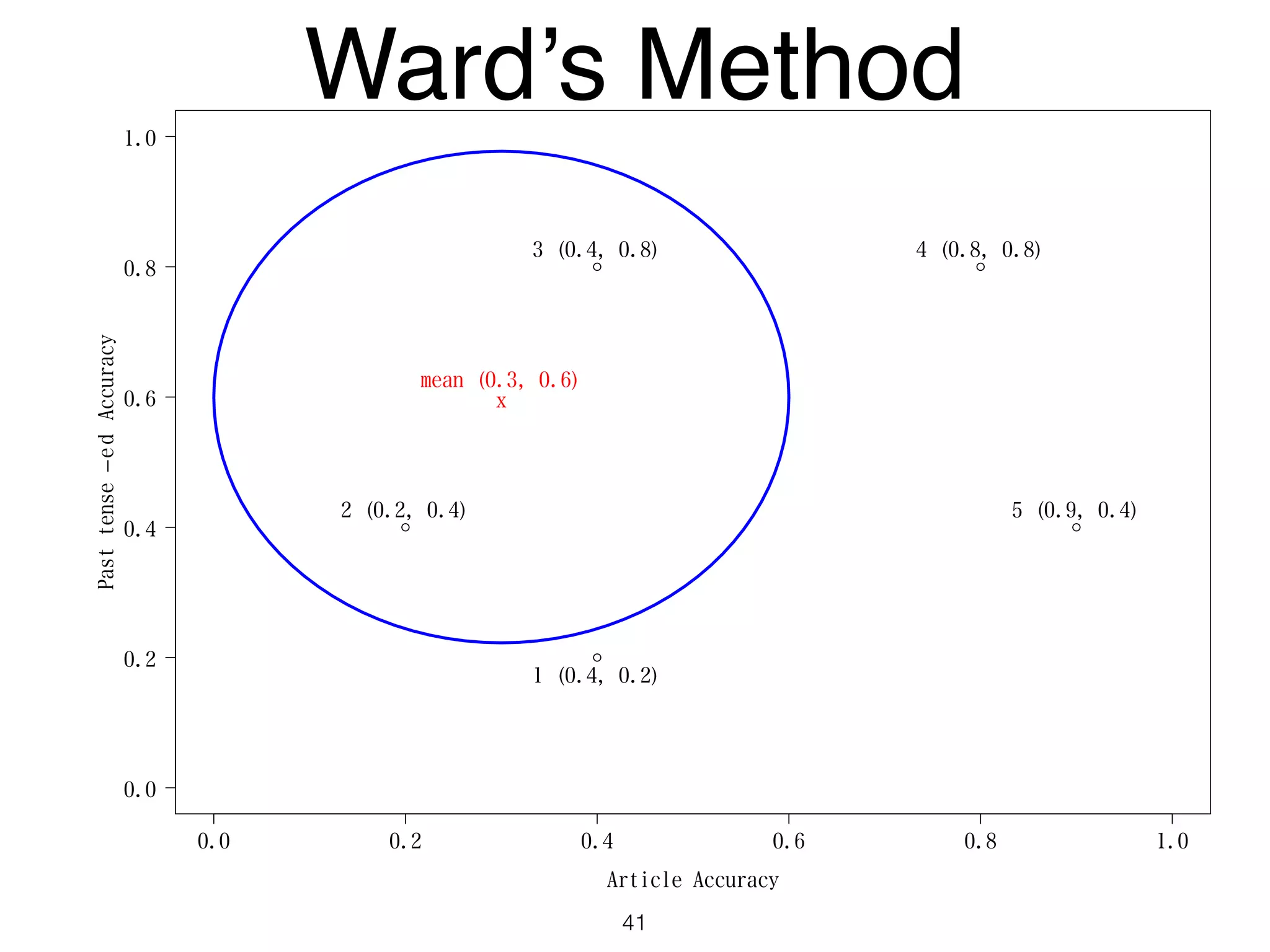
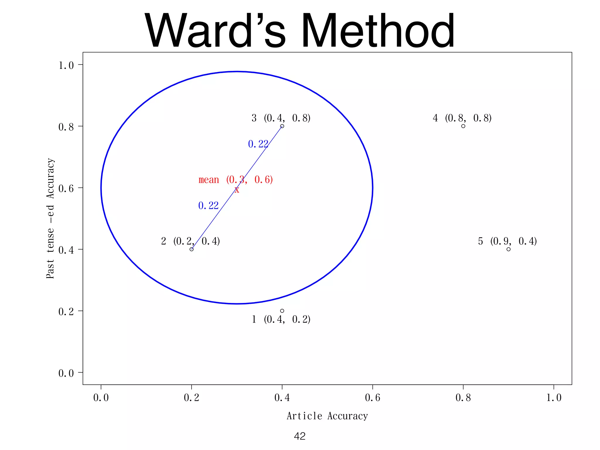
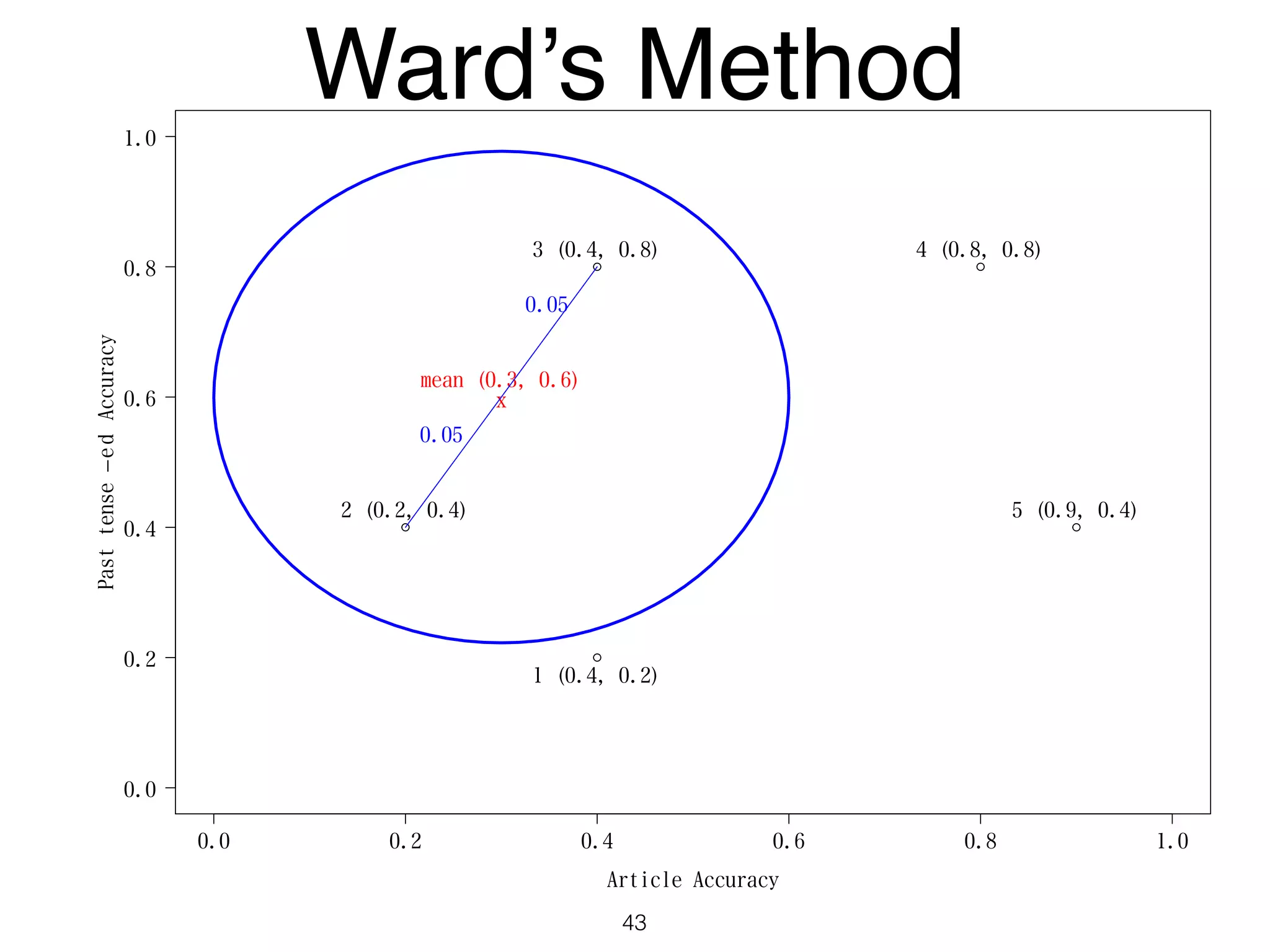
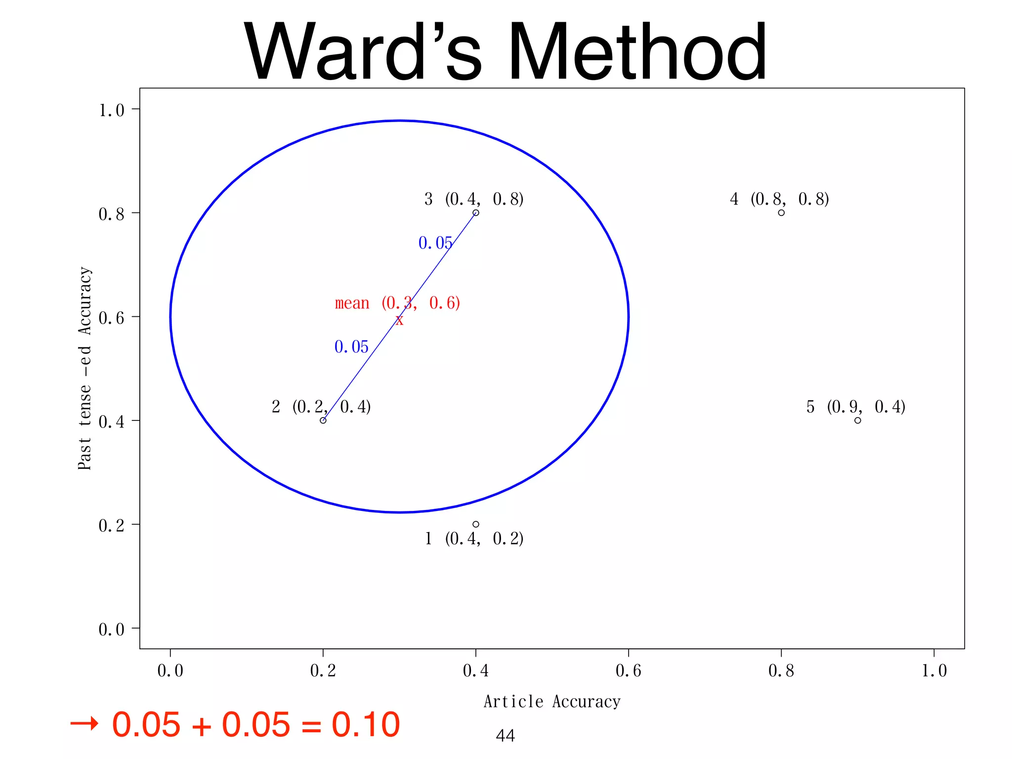


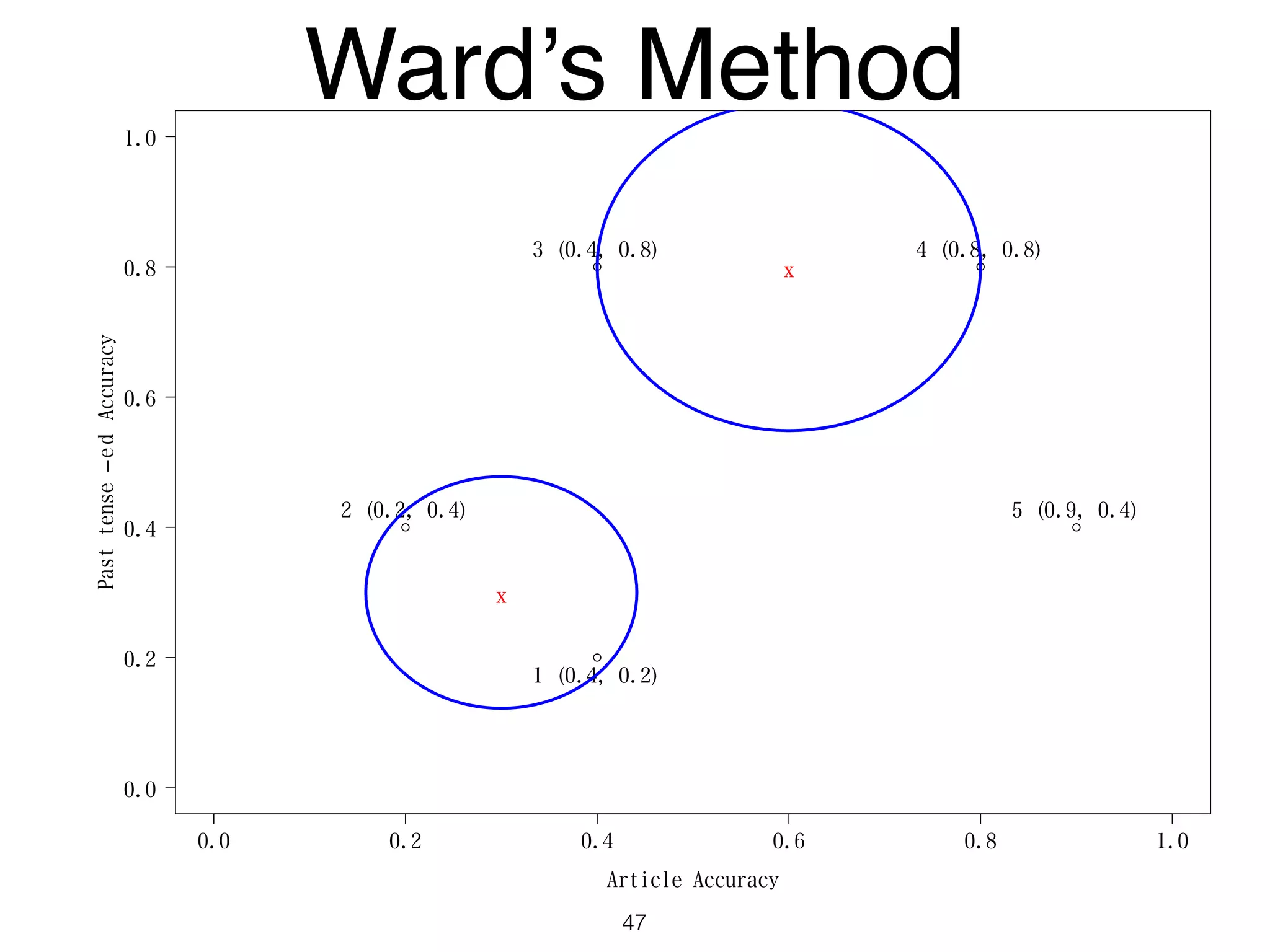
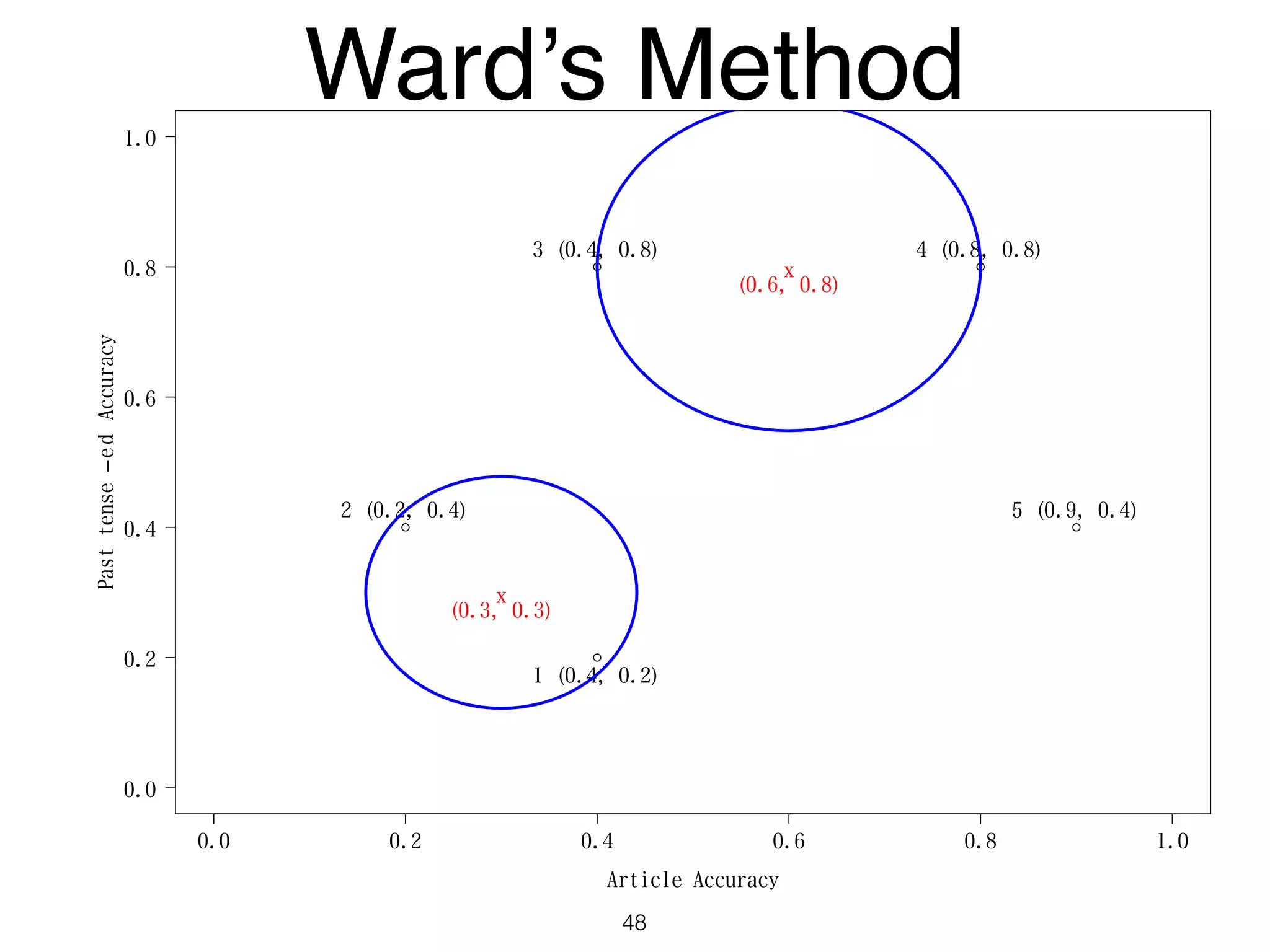
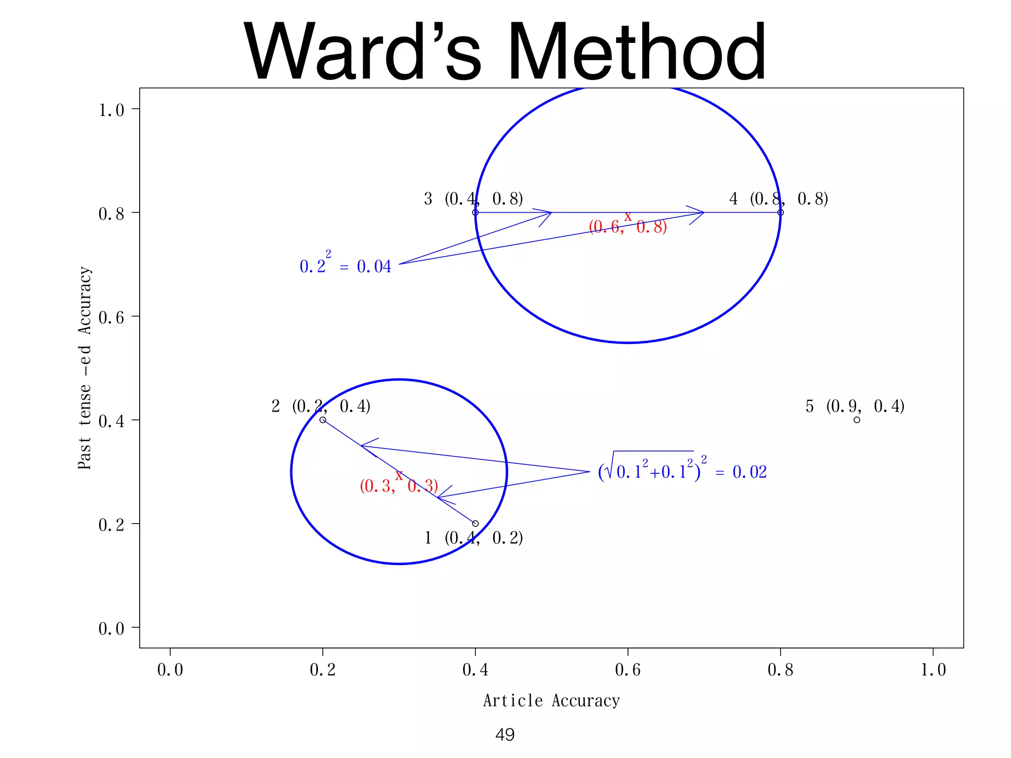
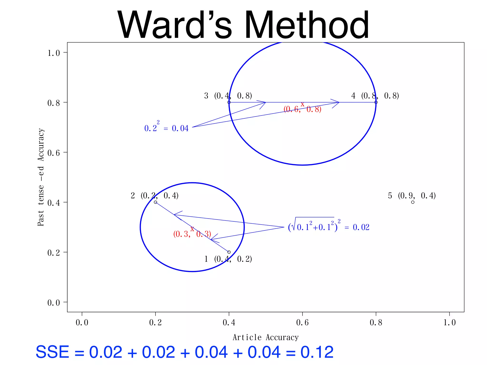
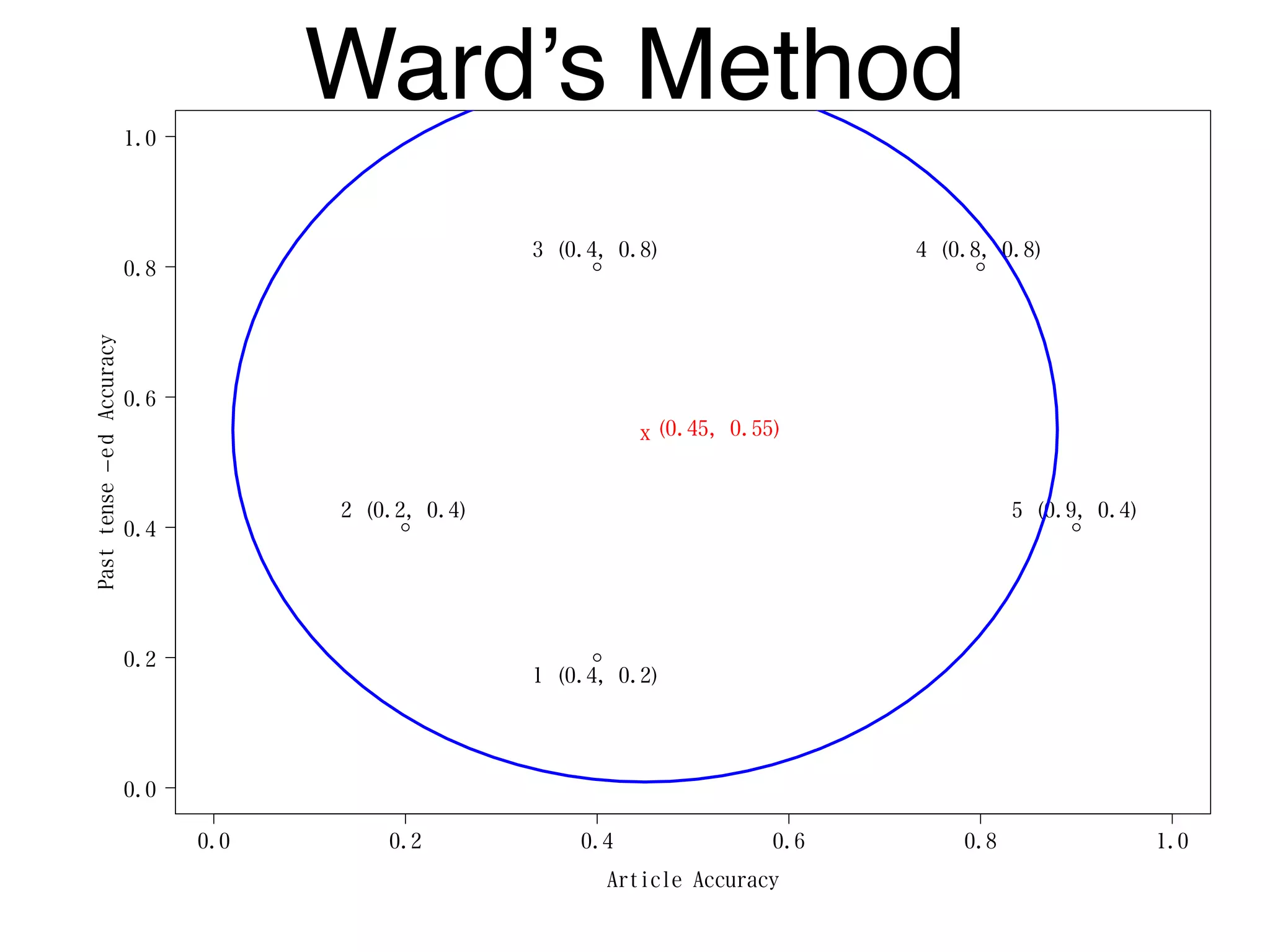
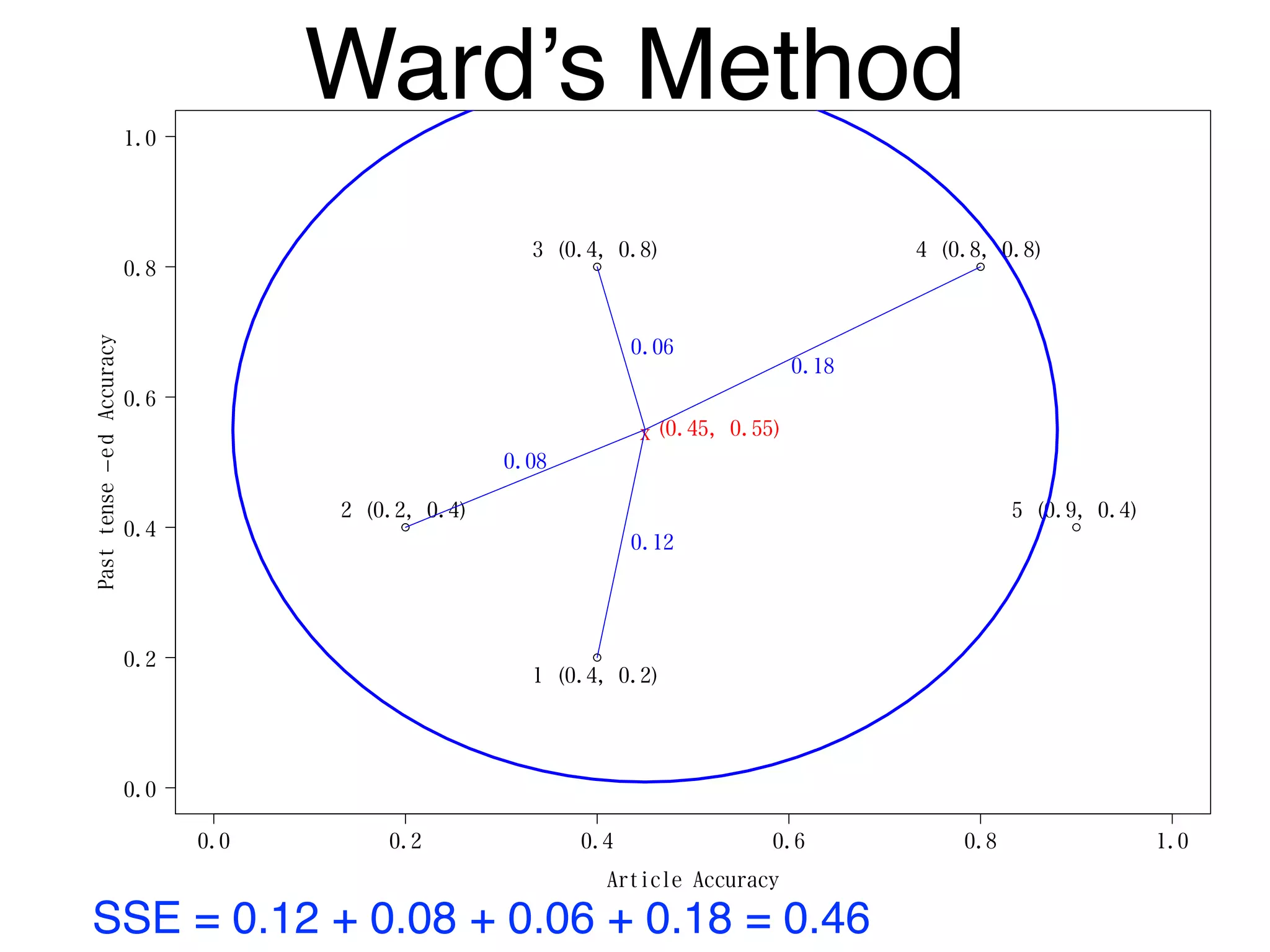

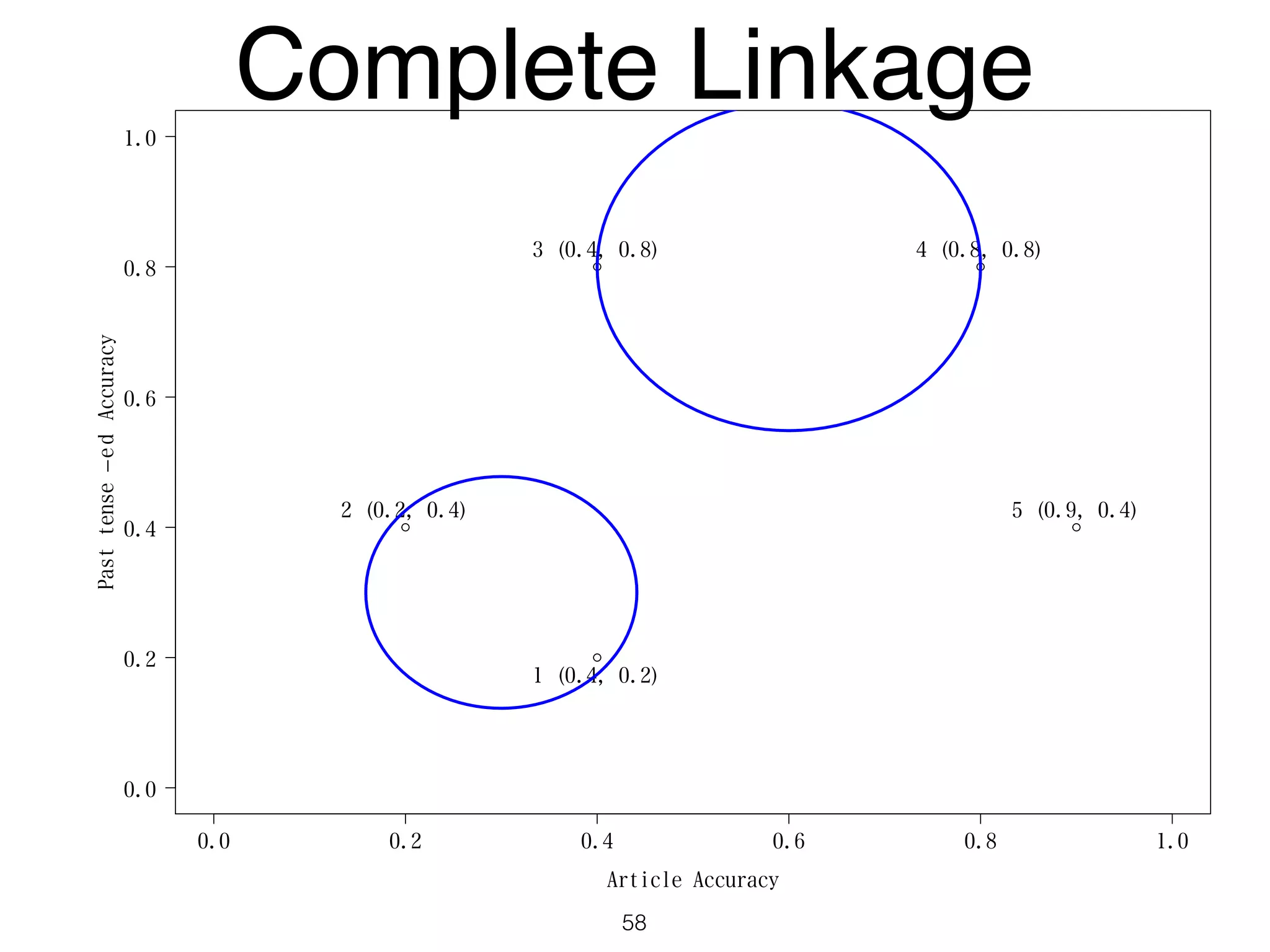
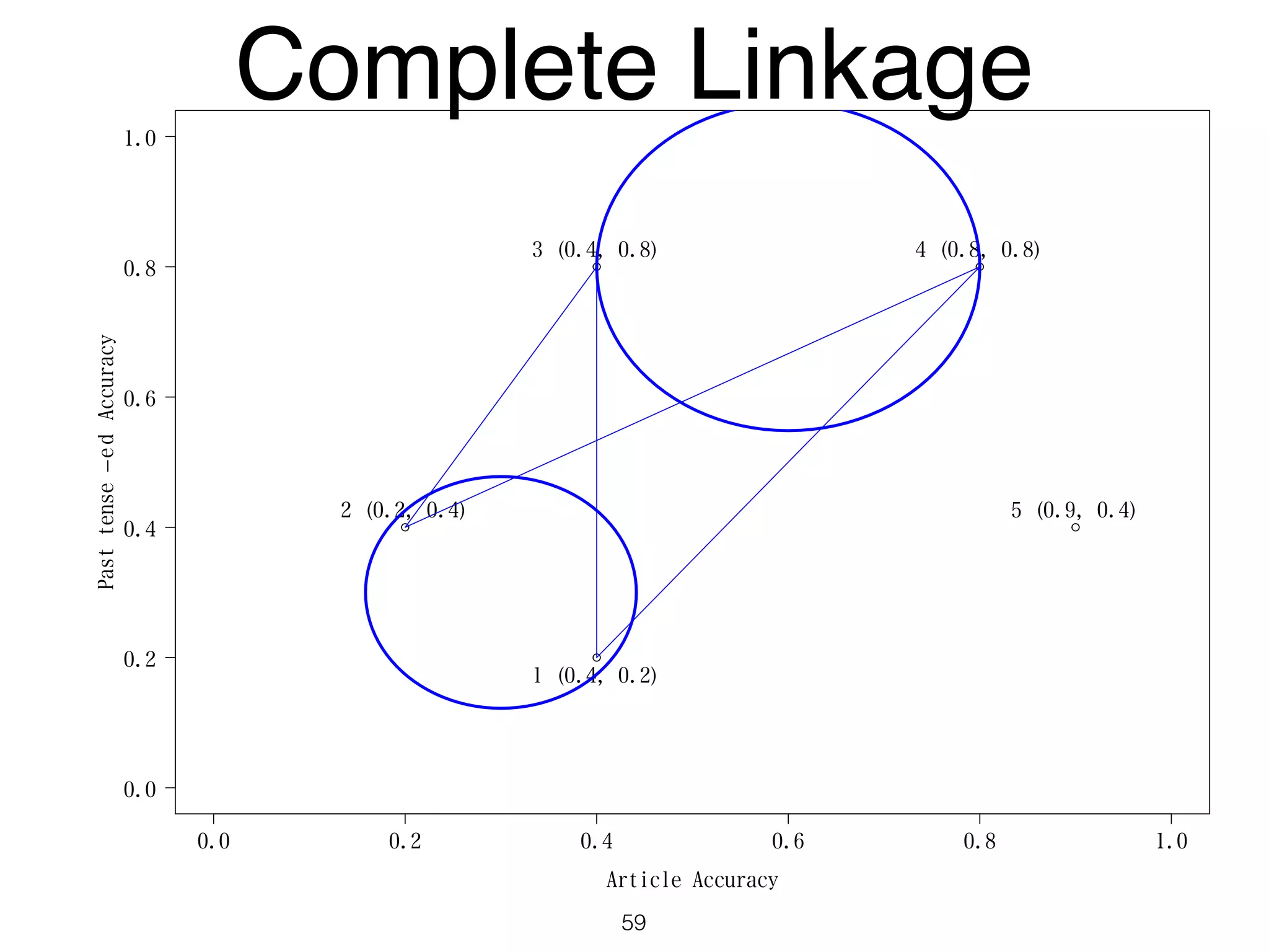
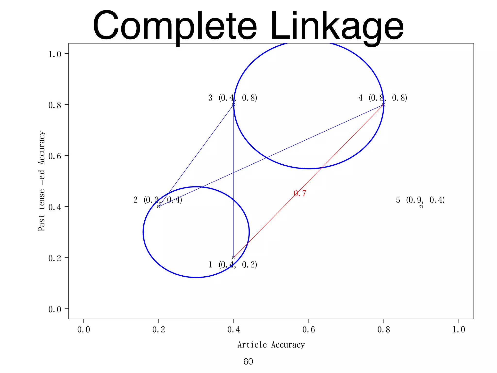
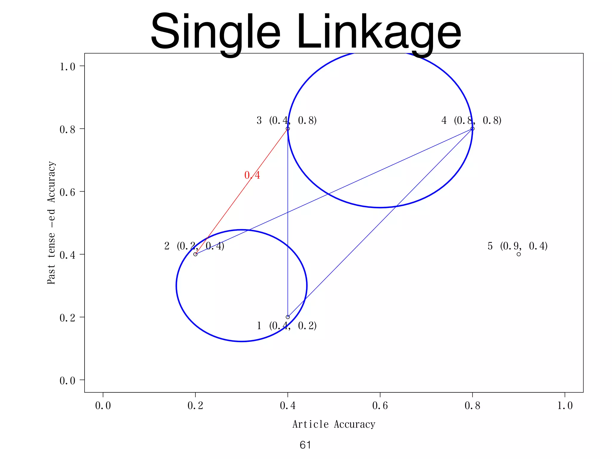
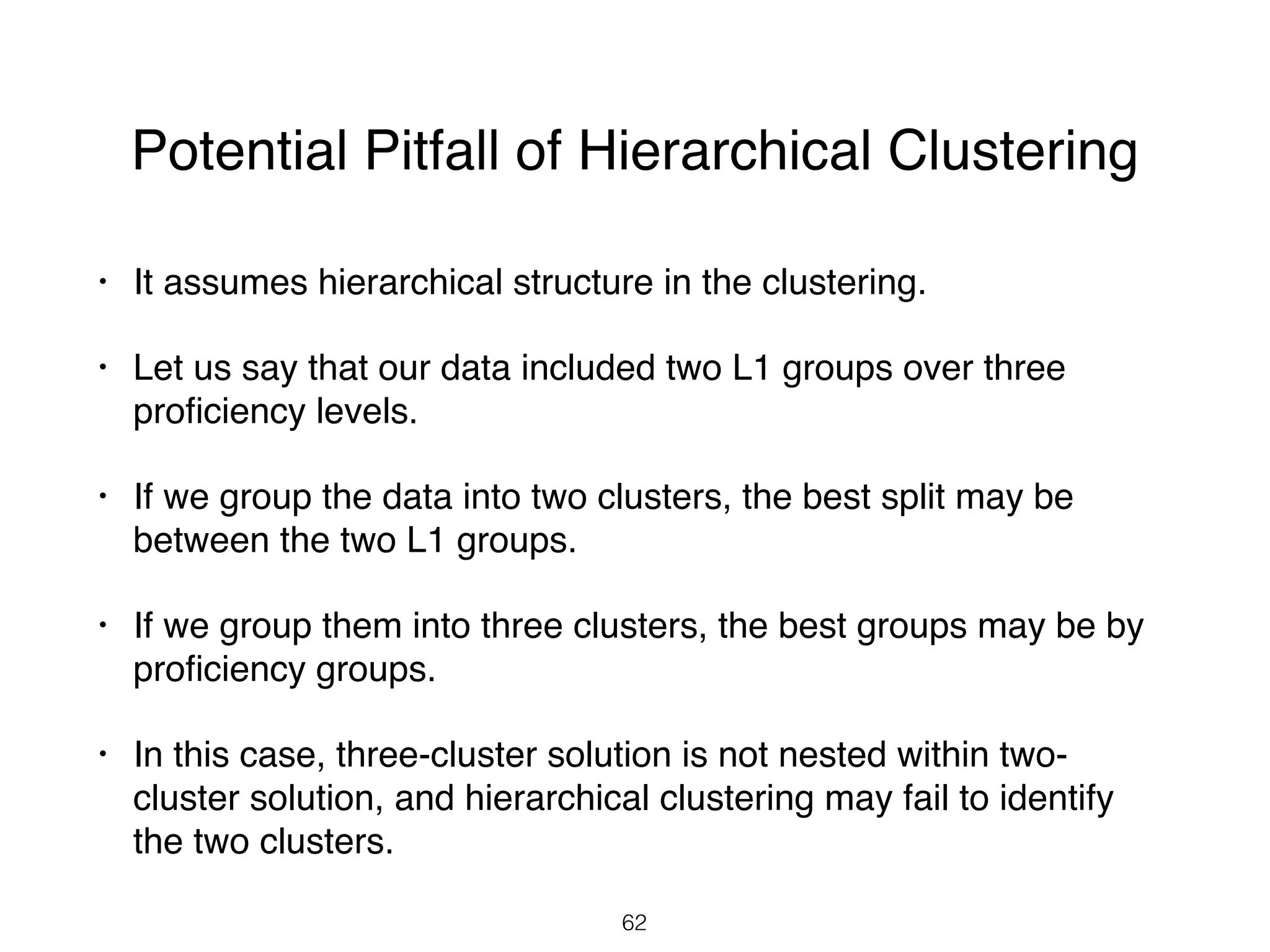
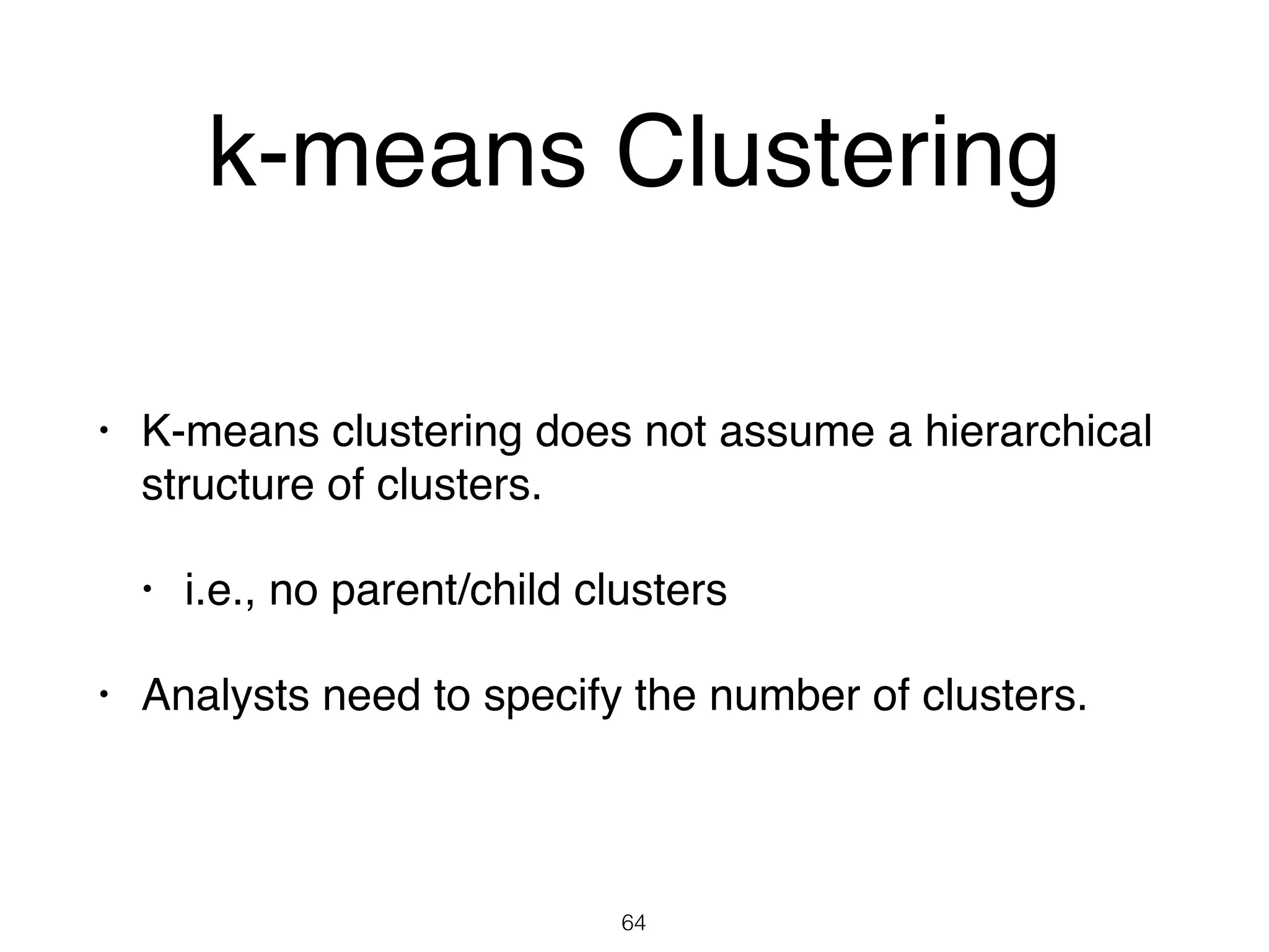
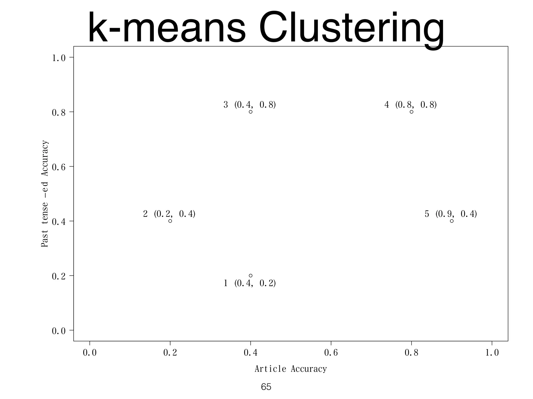

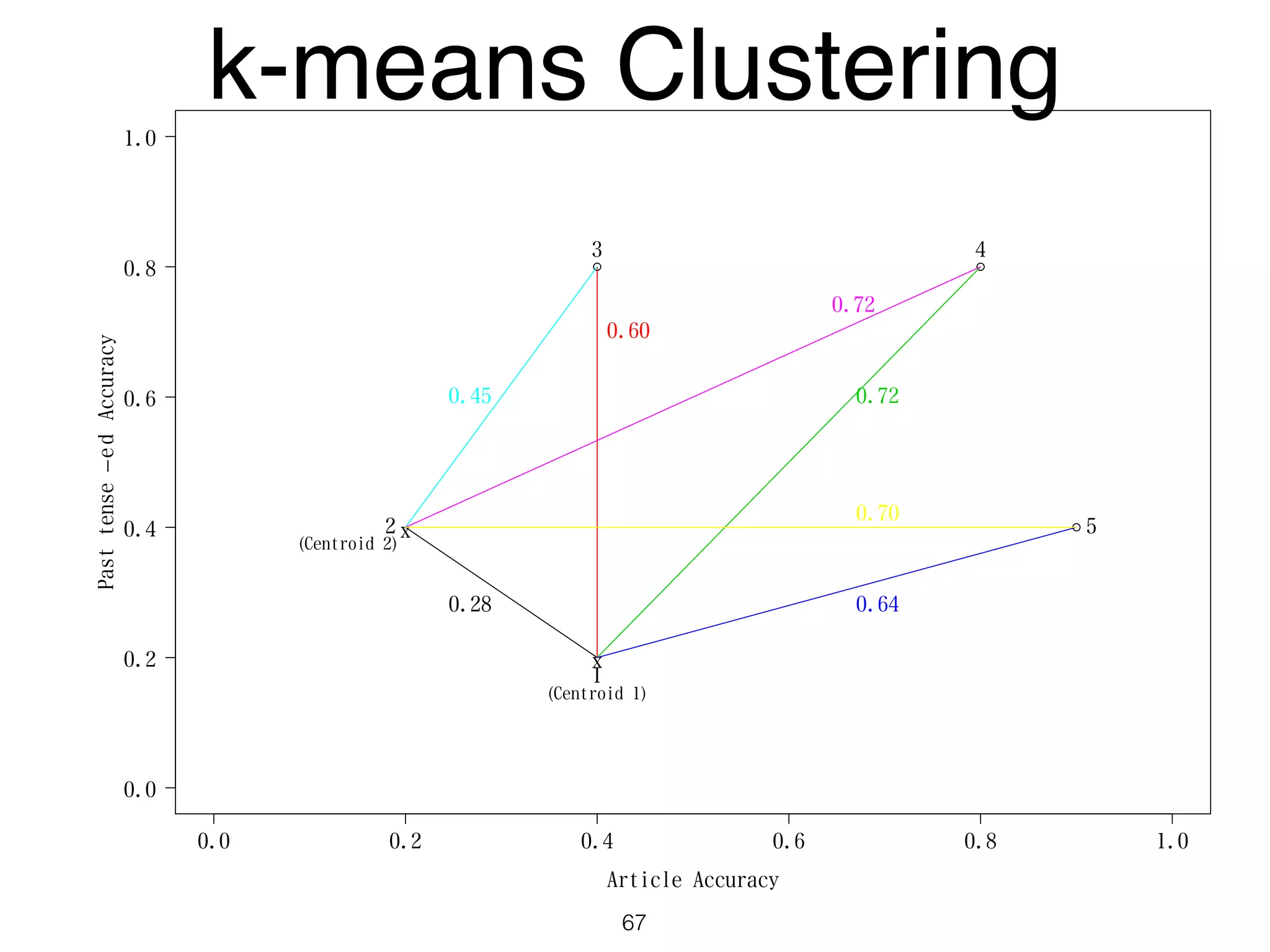
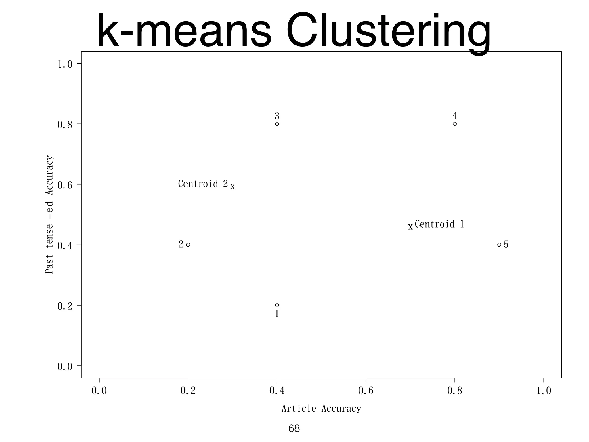
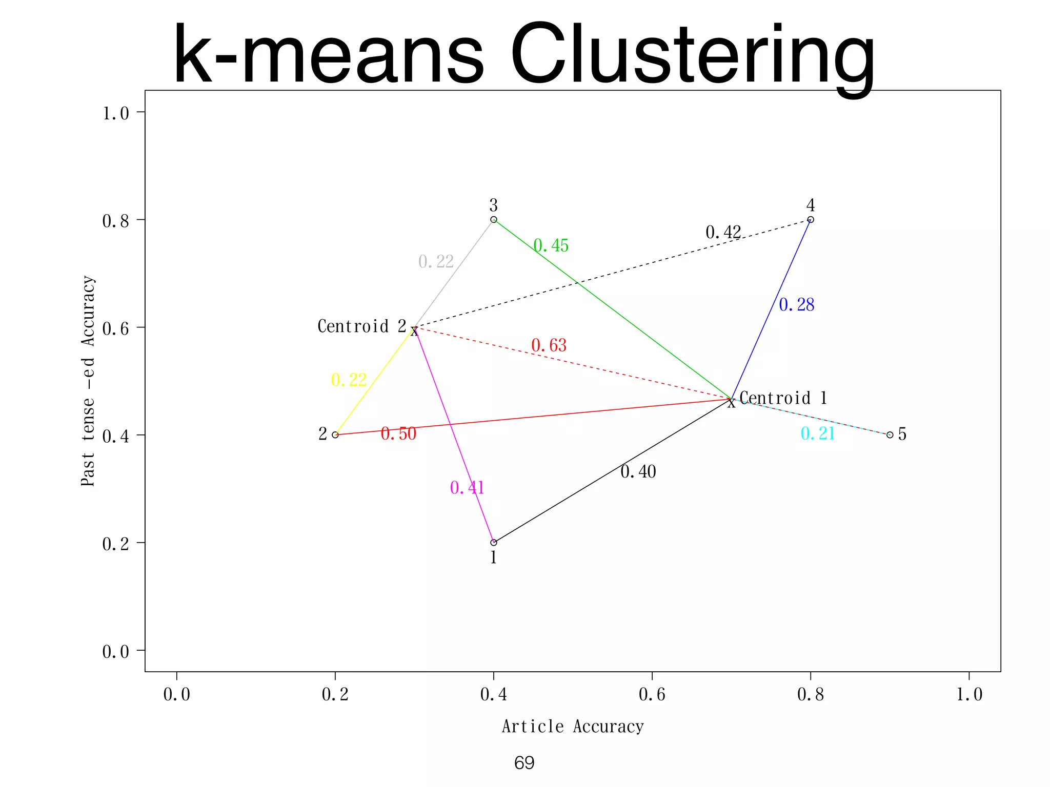


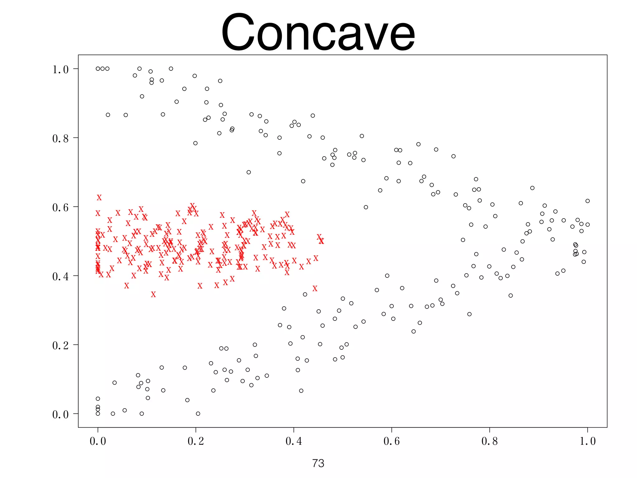


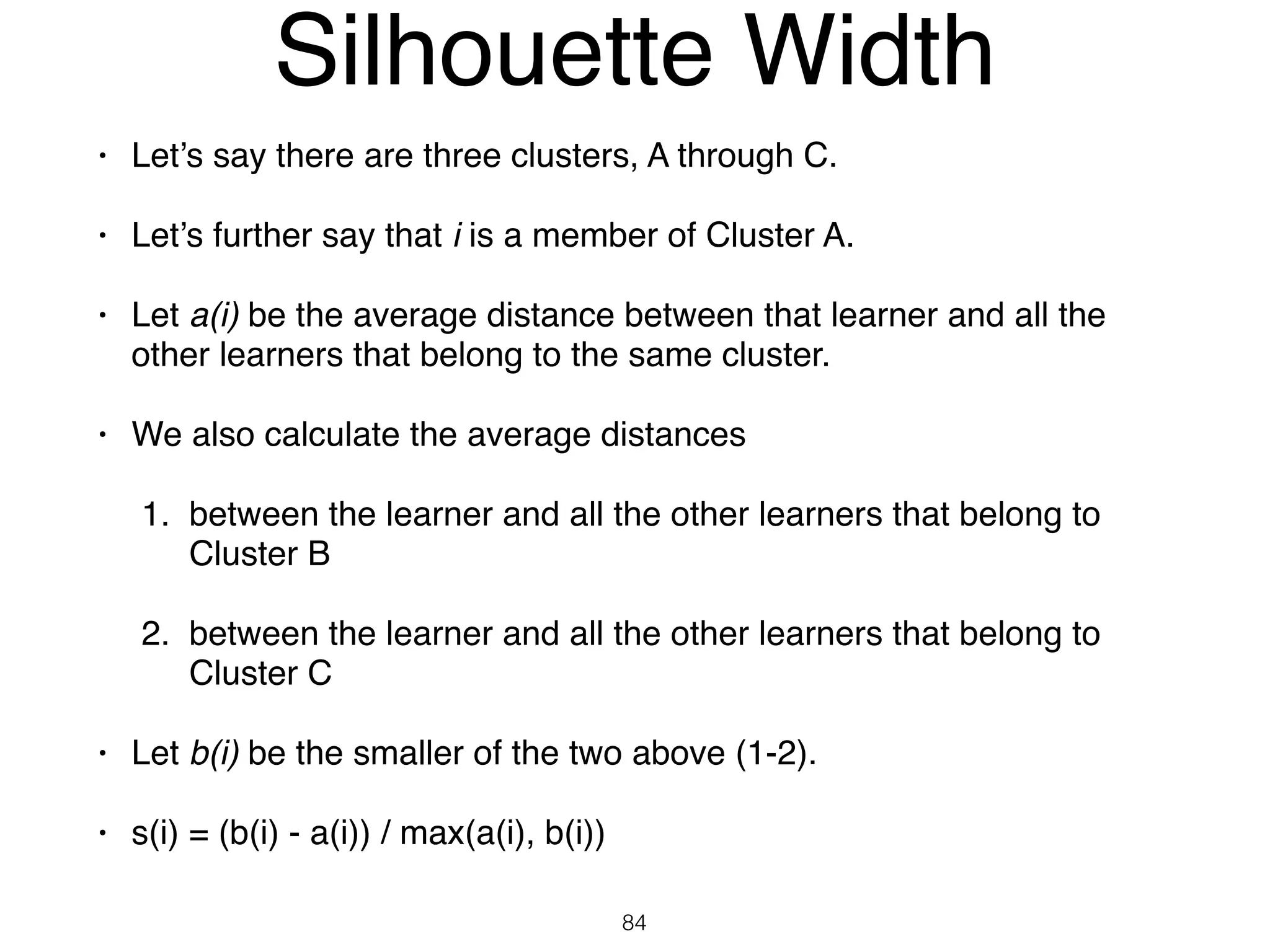


The document discusses clustering methods in R, emphasizing cluster analysis to identify groups based on similarity among data points. Various distance measures and clustering algorithms, such as agglomerative hierarchical clustering and k-means, are examined, including techniques for calculating cluster similarity. The content is particularly focused on applications in second language acquisition, exploring typologies of learner profiles through statistical methods.


![Agentic Systems and Compliance - A brief intro [1.2]](https://cdn.slidesharecdn.com/ss_thumbnails/agenticsystemsandcompliace-1-251018025303-958a42ec-thumbnail.jpg?width=600ounds&width=560&fit=bounds)


![Matrix and determinant URT [Autosaved].pptx](https://cdn.slidesharecdn.com/ss_thumbnails/matrixanddeterminanturtautosaved-251018190340-9e6a6deb-thumbnail.jpg?width=600ounds&width=560&fit=bounds)

![RTP_AR_Basic_Learners' Workbook_KS2 [FOR REPRODUCTION] (1).pdf](https://cdn.slidesharecdn.com/ss_thumbnails/rtparbasiclearnersworkbookks2forreproduction1-251016024943-e51a16ac-thumbnail.jpg?width=600ounds&width=560&fit=bounds)

