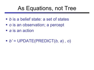
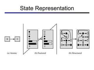
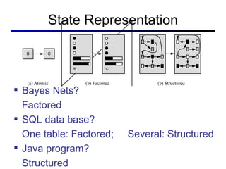
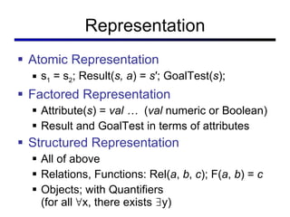
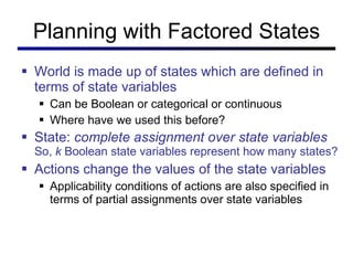
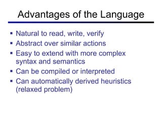
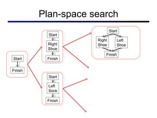
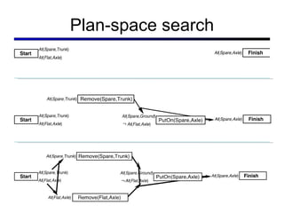
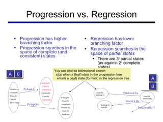
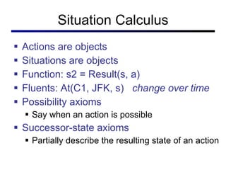
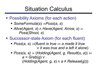
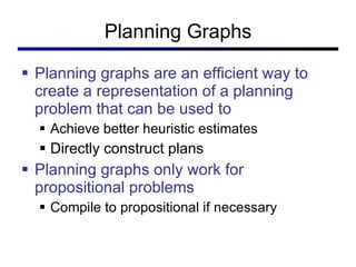
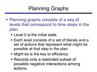
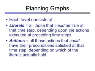
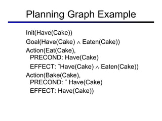
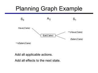
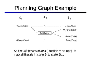
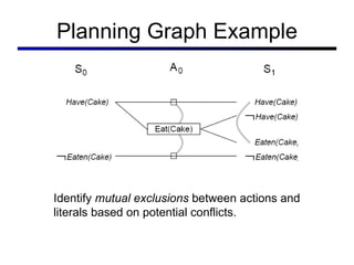
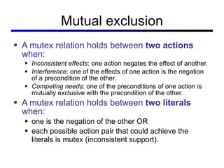
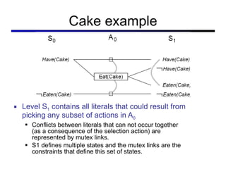
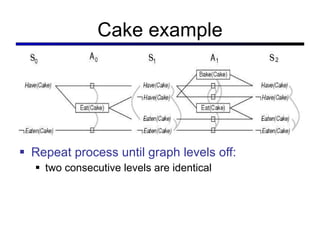
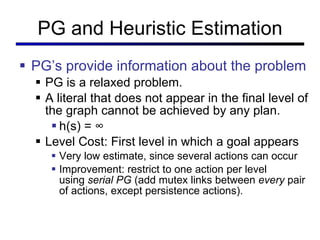
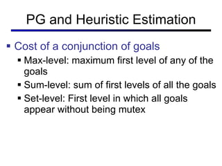
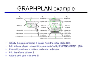
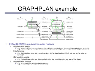
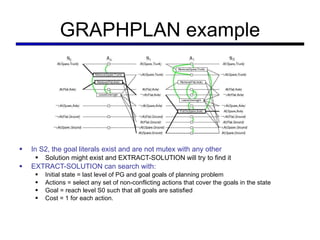
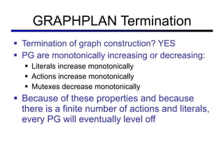
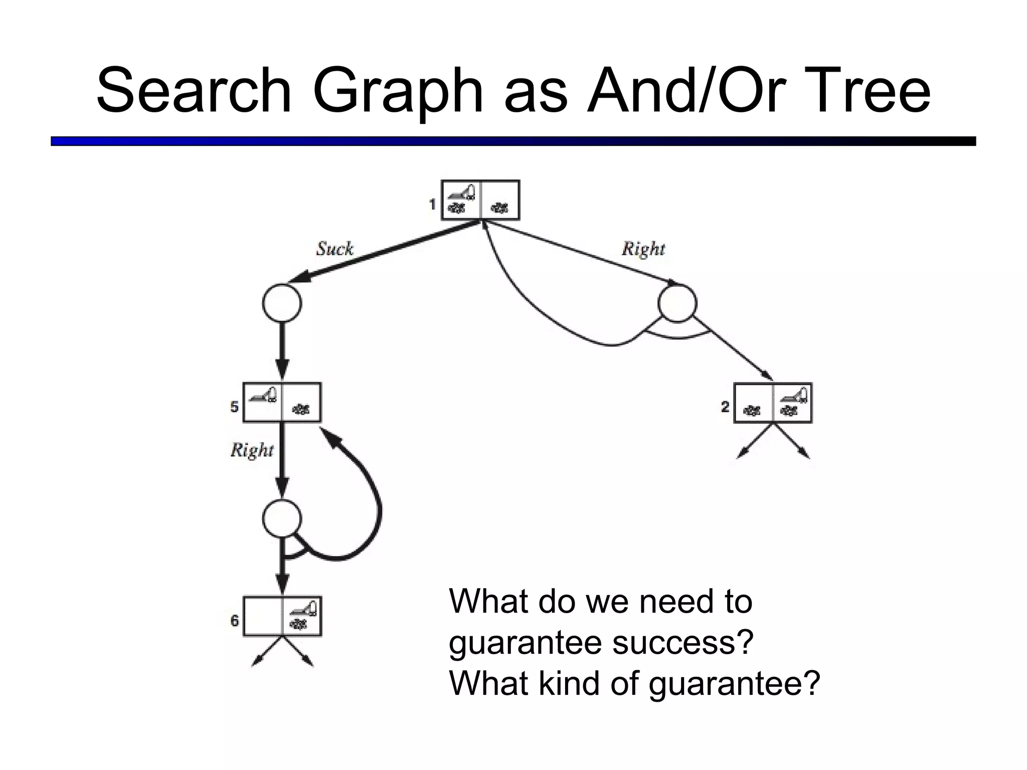
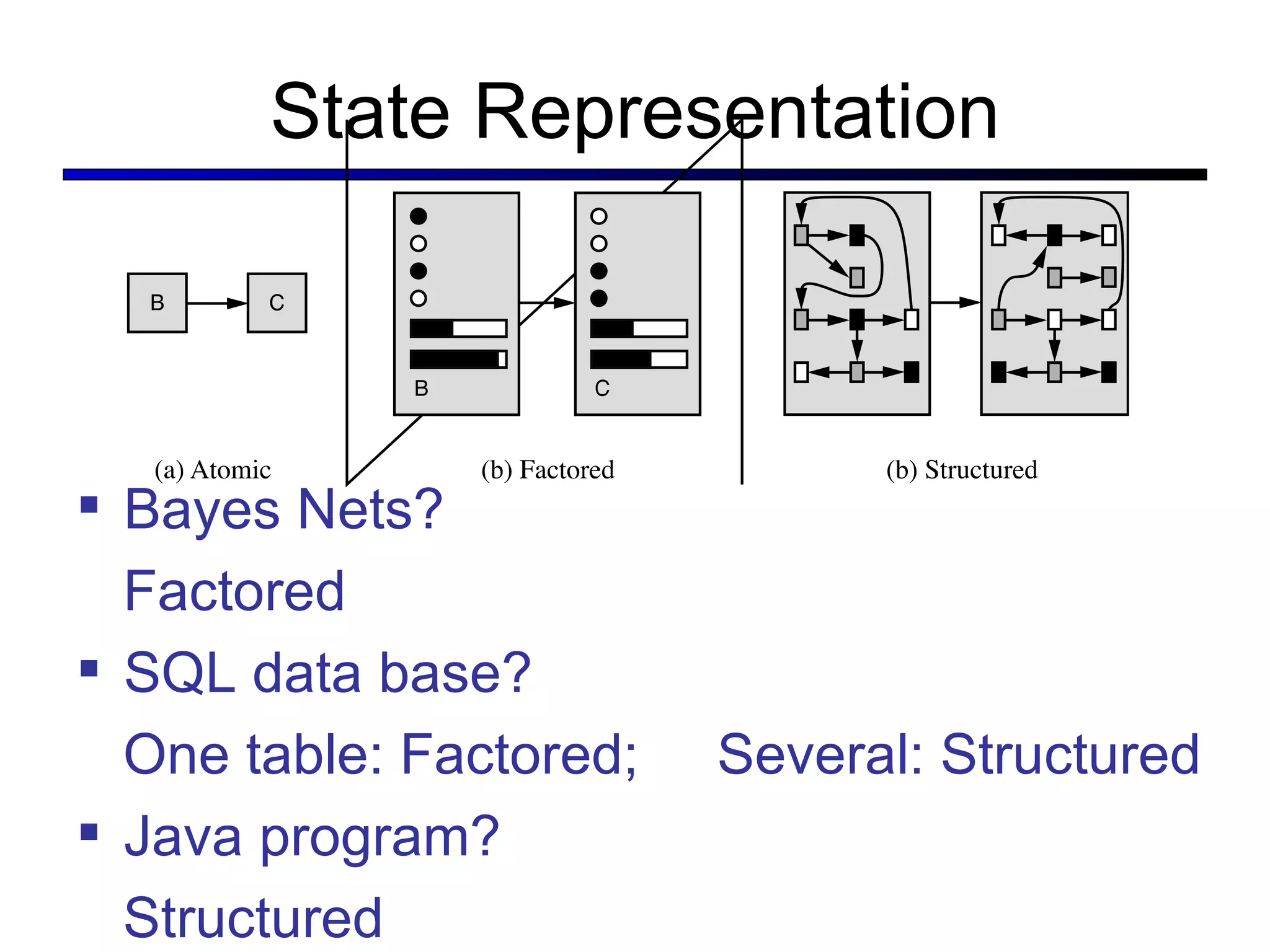
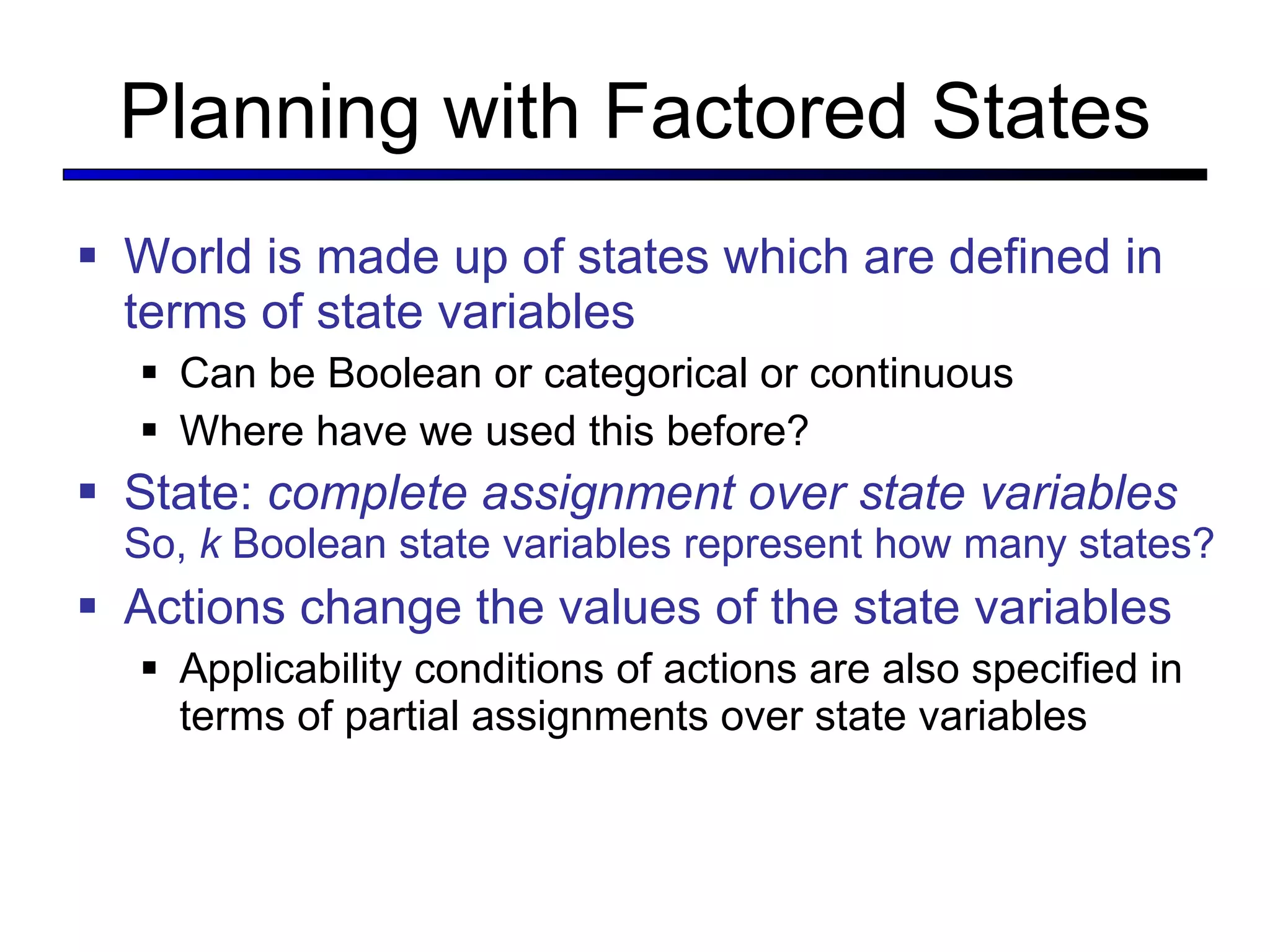
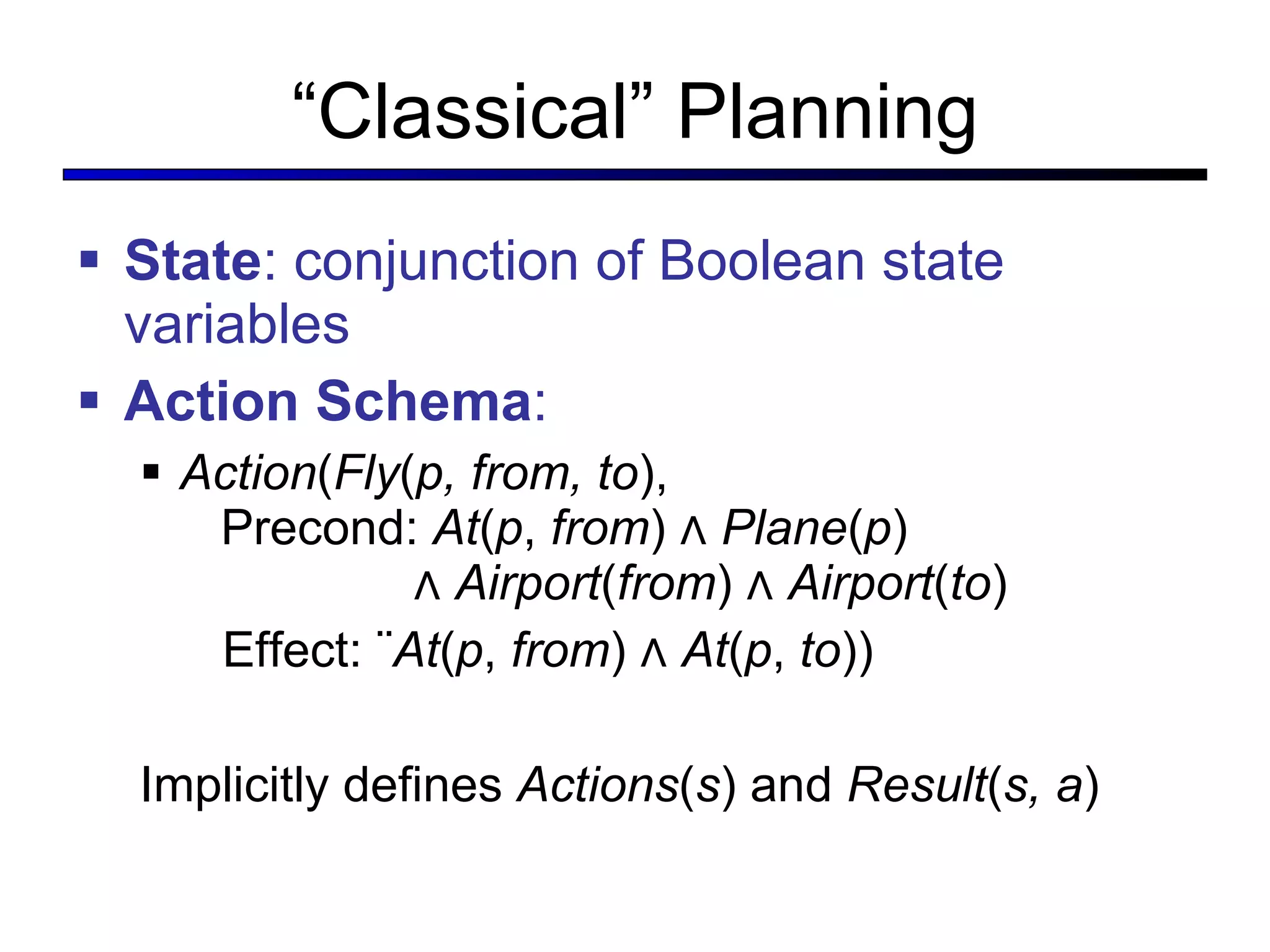
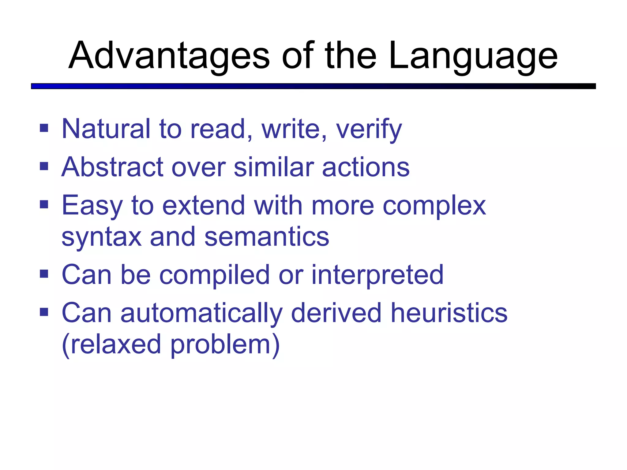
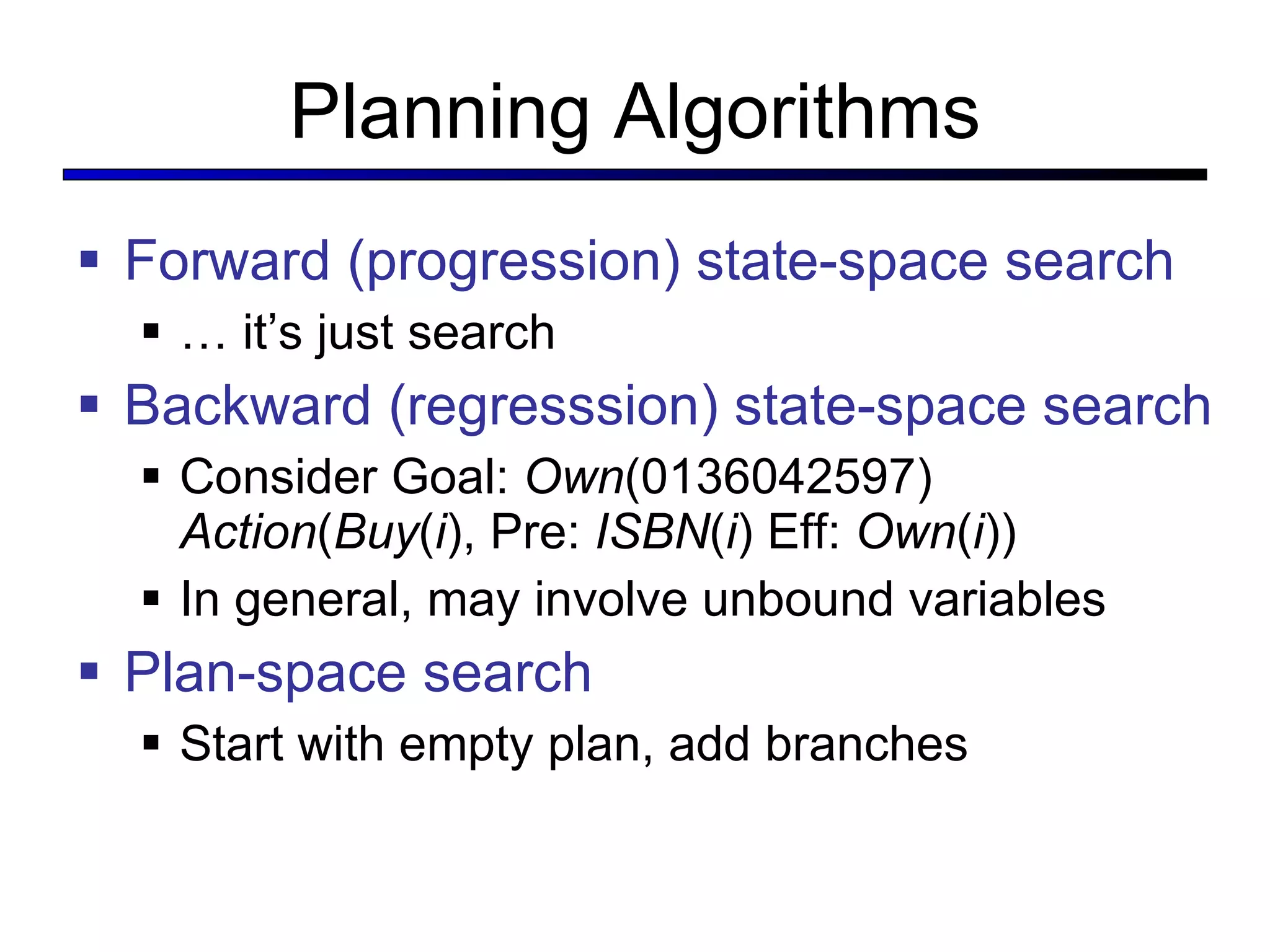
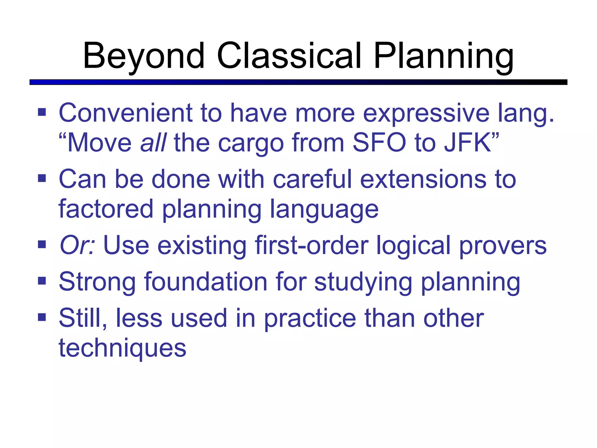
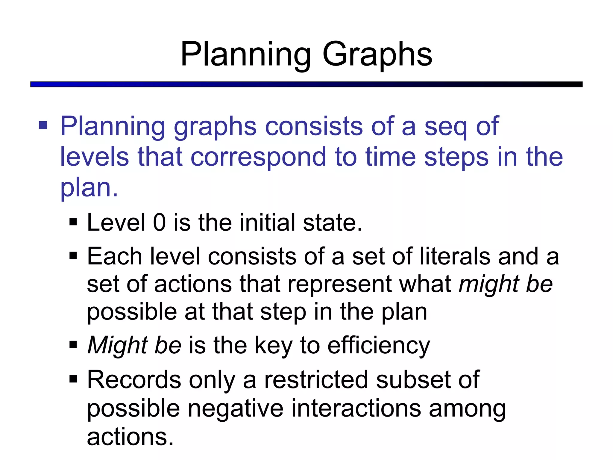
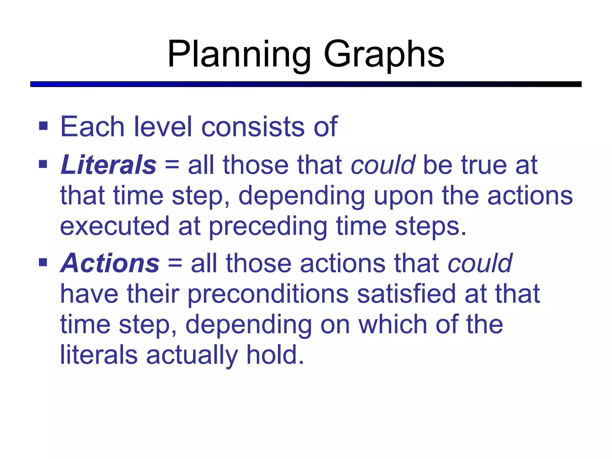
This document summarizes key concepts in artificial intelligence planning and logic. It discusses representations like atomic, factored, and structured states. Planning approaches include state-space search, planning graphs, and situation calculus. Factored representations allow more flexible and hierarchical plans using relations between state variables. Planning graphs efficiently represent possible plan states and actions to derive heuristic estimates and extract plans.
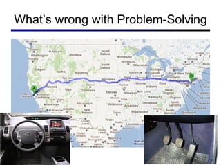
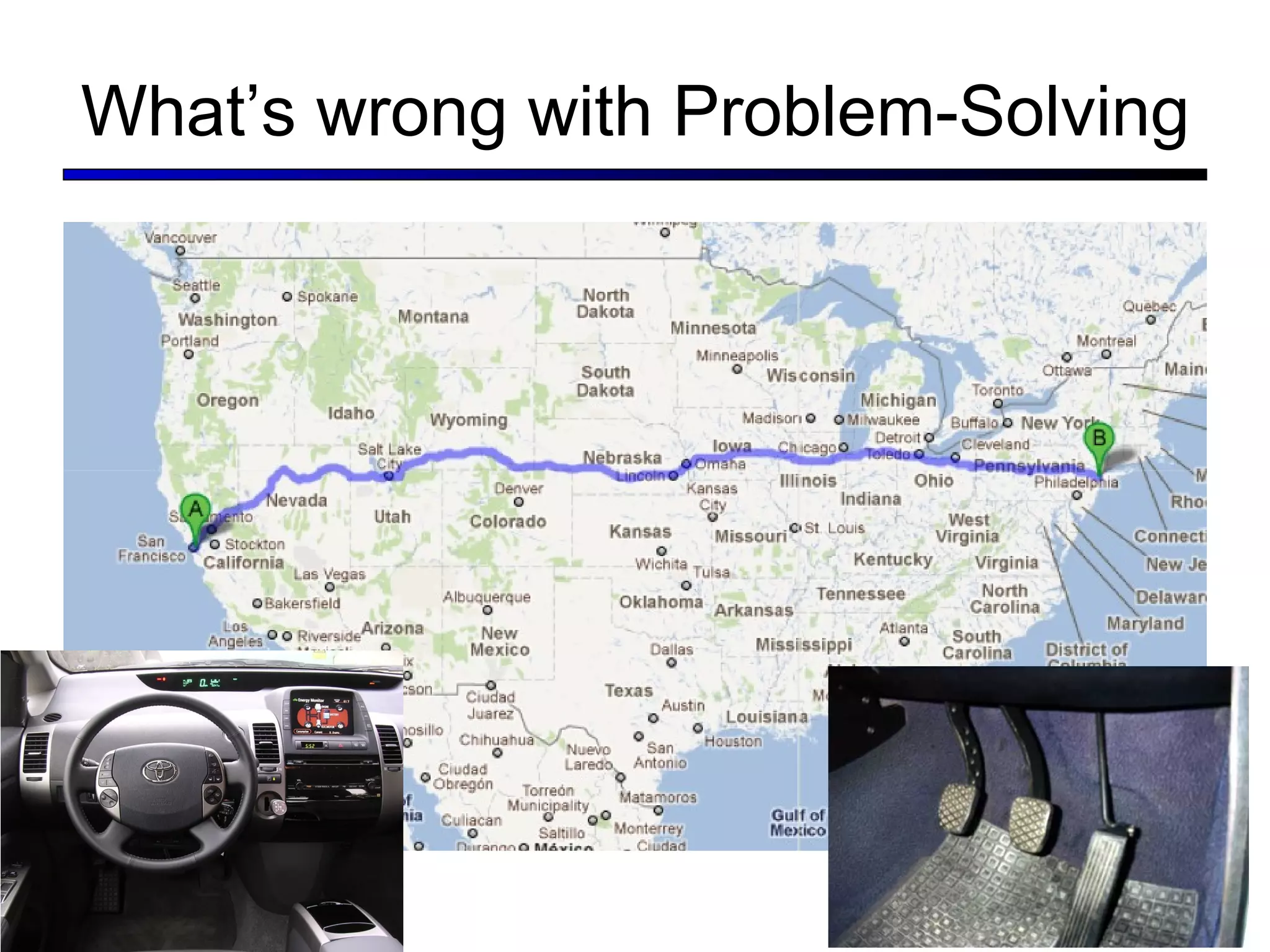
![What’s wrong with Problem-Solving Plan: [Forward, Forward, Forward, …]](https://image.slidesharecdn.com/cs221-lecture7-fall11-111104223435-phpapp01/85/Cs221-lecture7-fall11-4-320.jpg)

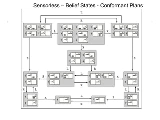
![Slippery wheels Planning and Sensing in Partially Observable and Stochastic World What is a plan to achieve all states clean? [1: Suck ; 2: Right ; ( if A : goto 2); 3: Suck ] also written as [ Suck ; ( while A : Right ); Suck ] Observe only local square; Suck is determ. R/L are stoch.; may fail to move](https://image.slidesharecdn.com/cs221-lecture7-fall11-111104223435-phpapp01/85/Cs221-lecture7-fall11-10-320.jpg)
![Kindergarten world: dirt may appear anywhere at any time, But actions are guaranteed to work. b1 b3 =UPDATE( b1 ,[ A,Clean ]) b5 = UPDATE( b4,… ) b2 =PREDICT( b1, Suck ) b4 =PREDICT( b3 , Right )](https://image.slidesharecdn.com/cs221-lecture7-fall11-111104223435-phpapp01/85/Cs221-lecture7-fall11-13-320.jpg)


![Situations as Result of Action Situation Calculus First-order Logic ∃s, p : Goal(s) ∧ s = Result(s0, p) s = Result(s, []) Result(s, [a,b,…]) = Result(Result(s, a), [b,…])](https://image.slidesharecdn.com/cs221-lecture7-fall11-111104223435-phpapp01/85/Cs221-lecture7-fall11-37-320.jpg)

![The GRAPHPLAN Algorithm Extract a solution directly from the PG function GRAPHPLAN( problem ) return solution or failure graph INITIAL-PLANNING-GRAPH( problem ) goals GOALS[ problem ] loop do if goals all non-mutex in last level of graph then do solution EXTRACT-SOLUTION( graph, goals, LEN (graph) ) if solution failure then return solution else if NO-SOLUTION-POSSIBLE( graph ) then return failure graph EXPAND-GRAPH( graph, problem )](https://image.slidesharecdn.com/cs221-lecture7-fall11-111104223435-phpapp01/85/Cs221-lecture7-fall11-51-320.jpg)

![What’s wrong with Problem-Solving Plan: [Forward, Forward, Forward, …]](https://image.slidesharecdn.com/cs221-lecture7-fall11-111104223435-phpapp01/75/Cs221-lecture7-fall11-4-2048.jpg)
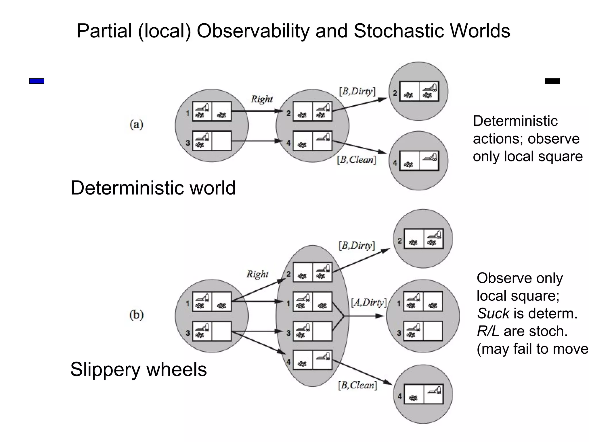
![Slippery wheels Planning and Sensing in Partially Observable and Stochastic World What is a plan to achieve all states clean? [1: Suck ; 2: Right ; ( if A : goto 2); 3: Suck ] also written as [ Suck ; ( while A : Right ); Suck ] Observe only local square; Suck is determ. R/L are stoch.; may fail to move](https://image.slidesharecdn.com/cs221-lecture7-fall11-111104223435-phpapp01/75/Cs221-lecture7-fall11-10-2048.jpg)
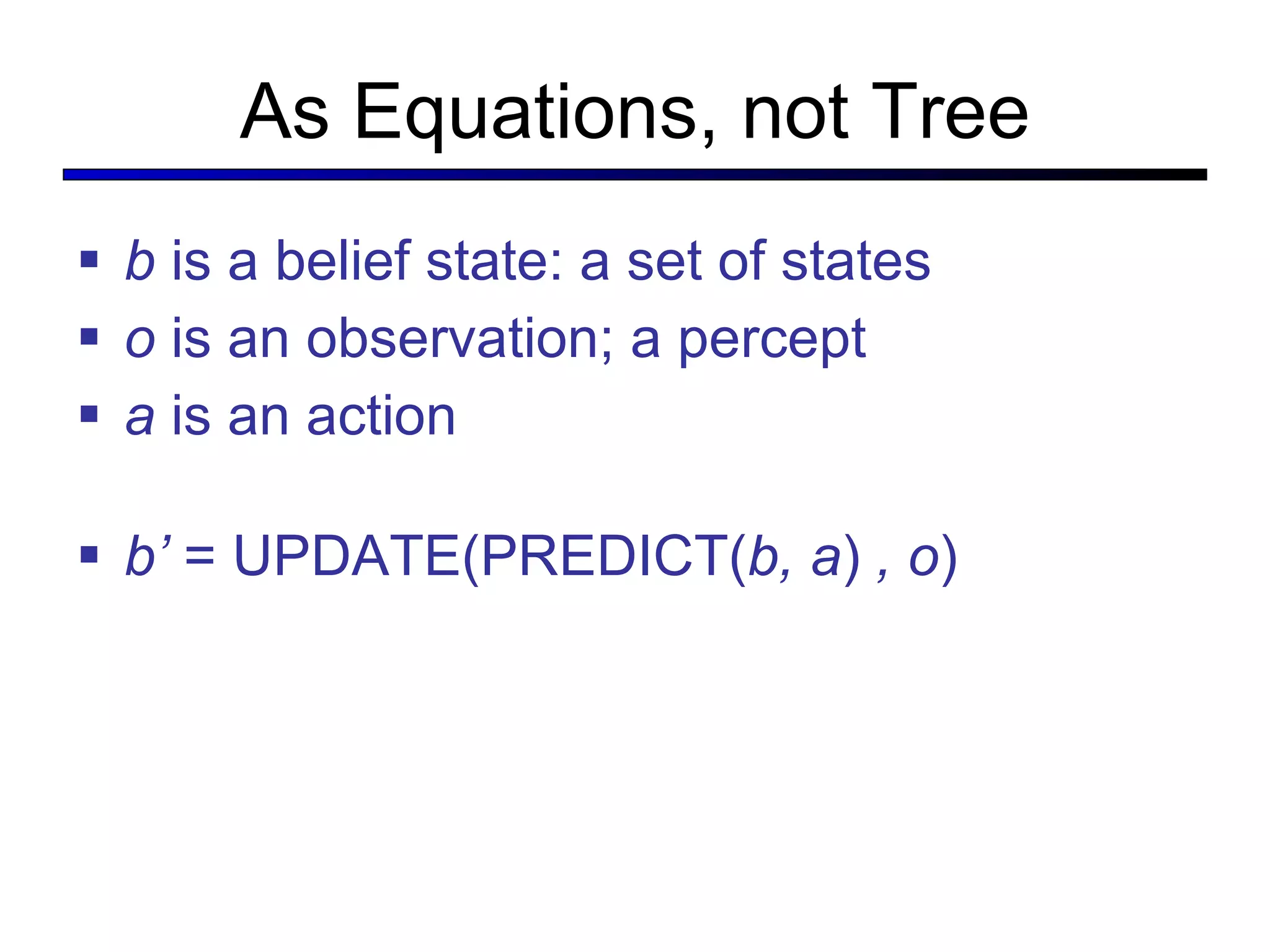
![Kindergarten world: dirt may appear anywhere at any time, But actions are guaranteed to work. b1 b3 =UPDATE( b1 ,[ A,Clean ]) b5 = UPDATE( b4,… ) b2 =PREDICT( b1, Suck ) b4 =PREDICT( b3 , Right )](https://image.slidesharecdn.com/cs221-lecture7-fall11-111104223435-phpapp01/75/Cs221-lecture7-fall11-13-2048.jpg)


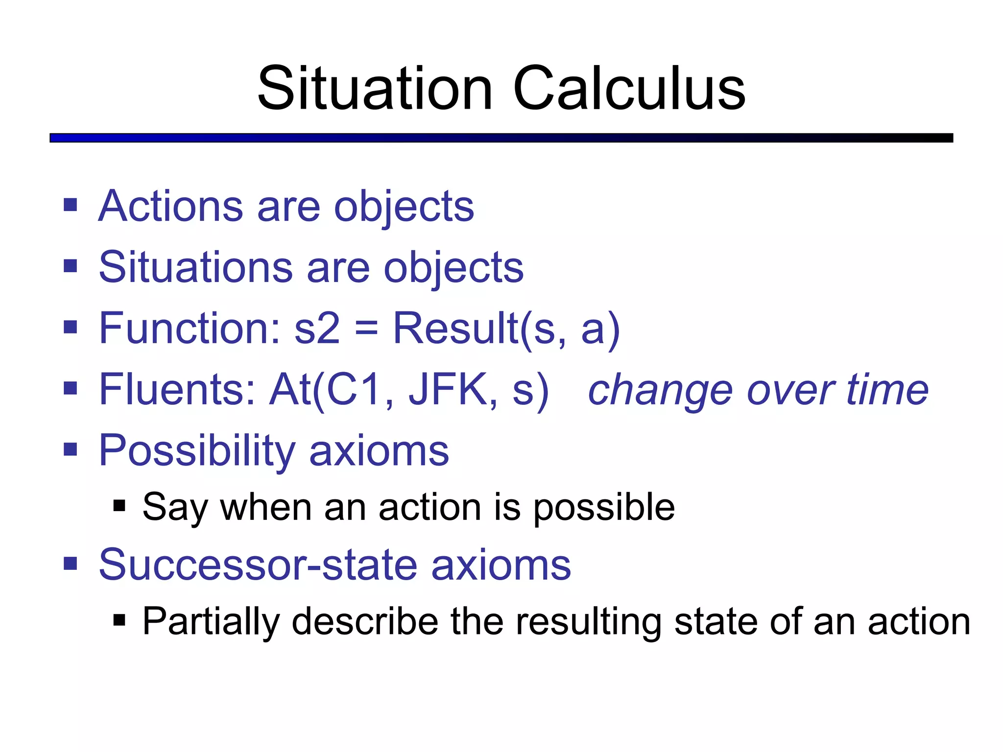

![Situations as Result of Action Situation Calculus First-order Logic ∃s, p : Goal(s) ∧ s = Result(s0, p) s = Result(s, []) Result(s, [a,b,…]) = Result(Result(s, a), [b,…])](https://image.slidesharecdn.com/cs221-lecture7-fall11-111104223435-phpapp01/75/Cs221-lecture7-fall11-37-2048.jpg)


![The GRAPHPLAN Algorithm Extract a solution directly from the PG function GRAPHPLAN( problem ) return solution or failure graph INITIAL-PLANNING-GRAPH( problem ) goals GOALS[ problem ] loop do if goals all non-mutex in last level of graph then do solution EXTRACT-SOLUTION( graph, goals, LEN (graph) ) if solution failure then return solution else if NO-SOLUTION-POSSIBLE( graph ) then return failure graph EXPAND-GRAPH( graph, problem )](https://image.slidesharecdn.com/cs221-lecture7-fall11-111104223435-phpapp01/75/Cs221-lecture7-fall11-51-2048.jpg)


![UiPath Automation Suite Installation (Hands-On) [2/3]](https://cdn.slidesharecdn.com/ss_thumbnails/automationsuitecommunitysession2-251015095633-a6d862f1-thumbnail.jpg?width=600ounds&width=560&fit=bounds)


