Download to read offline


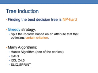


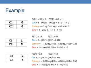


![Cost vs Accuracy
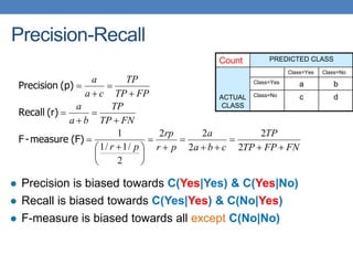
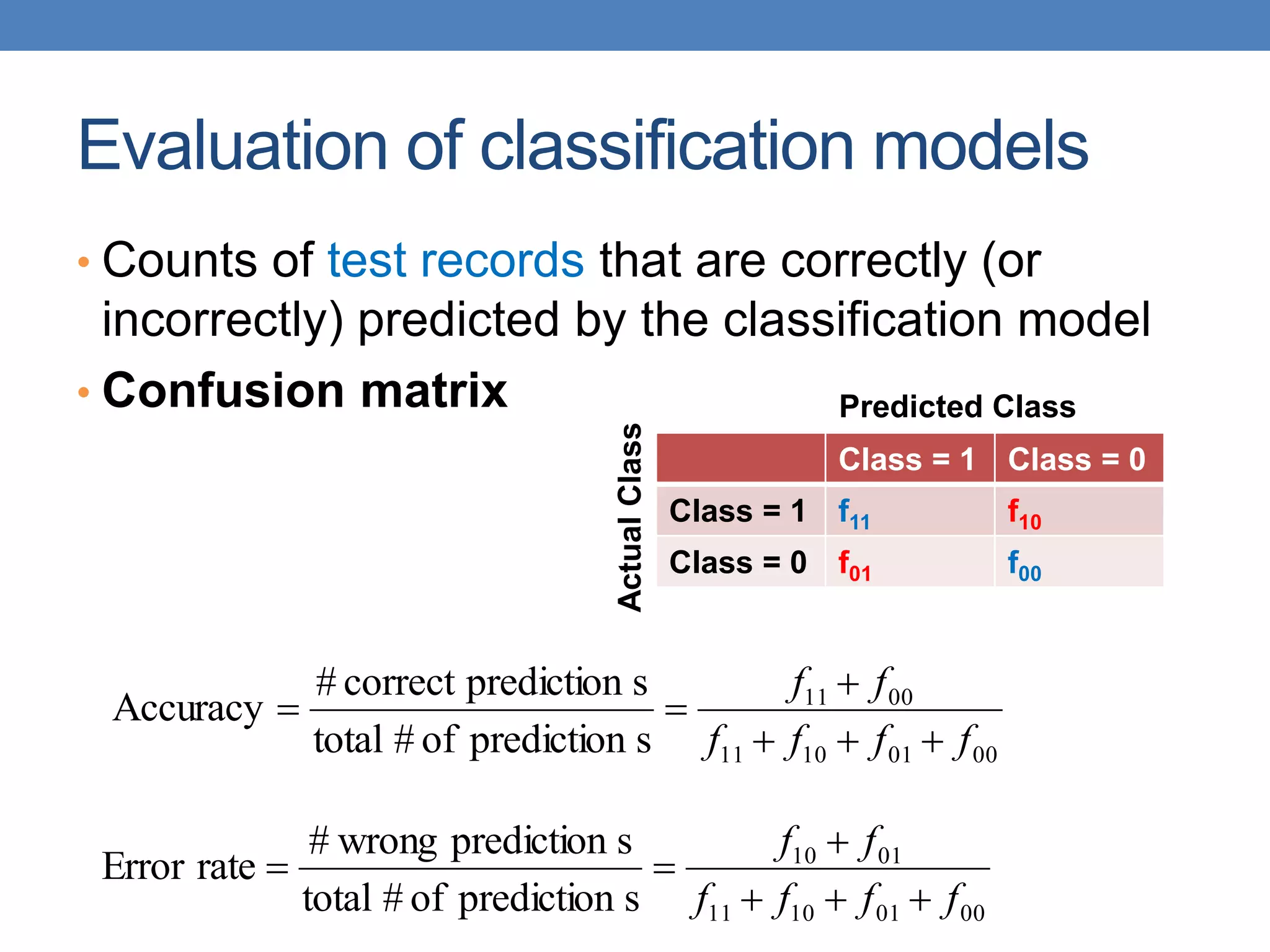
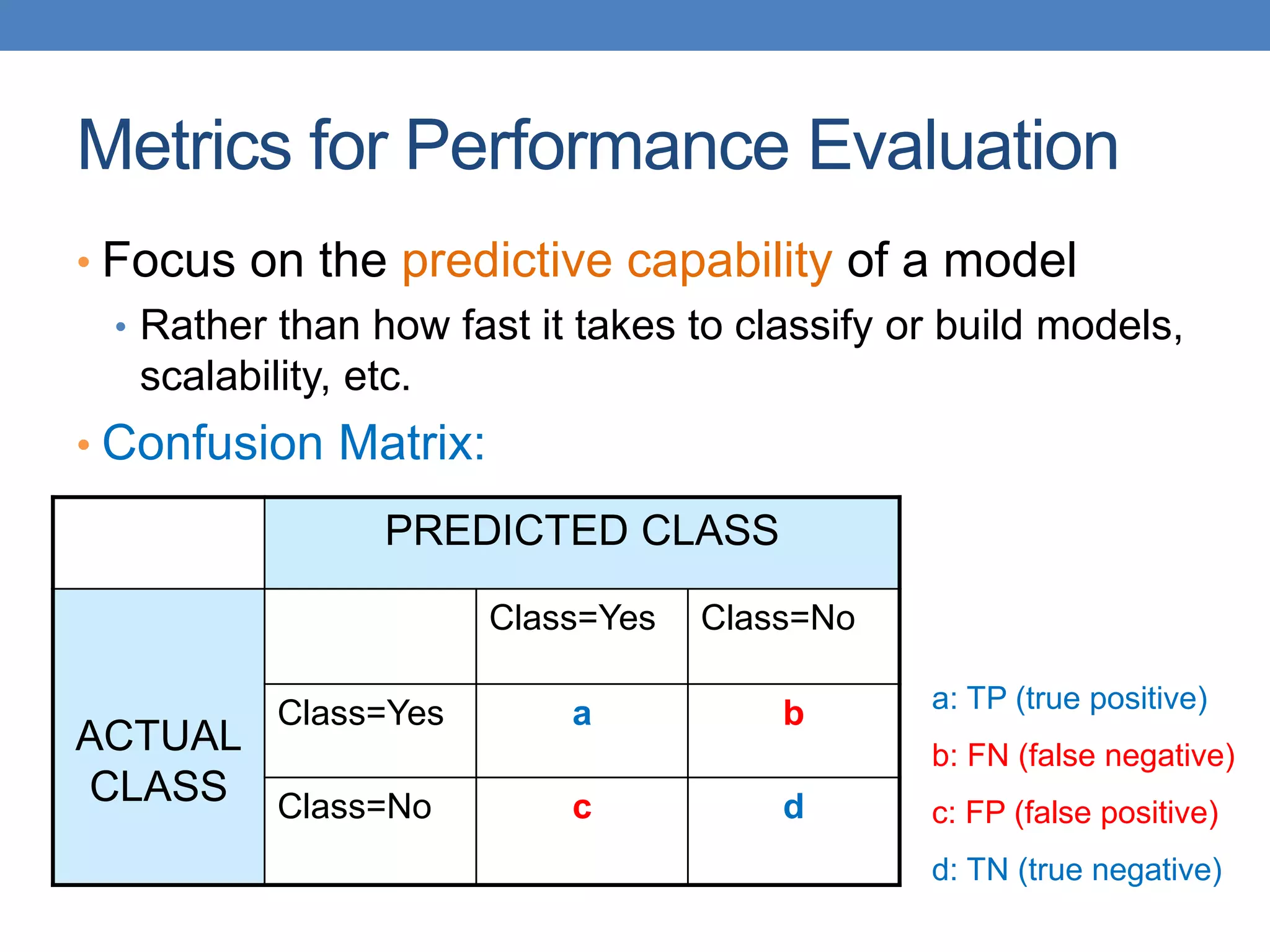
Count PREDICTED CLASS
ACTUAL
CLASS
Class=Yes Class=No
Class=Yes a b
Class=No c d
Cost PREDICTED CLASS
ACTUAL
CLASS
Class=Yes Class=No
Class=Yes p q
Class=No q p
N = a + b + c + d
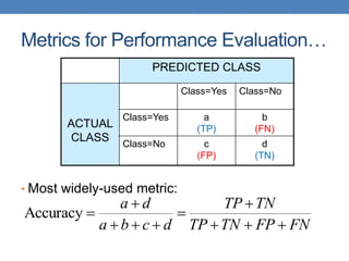
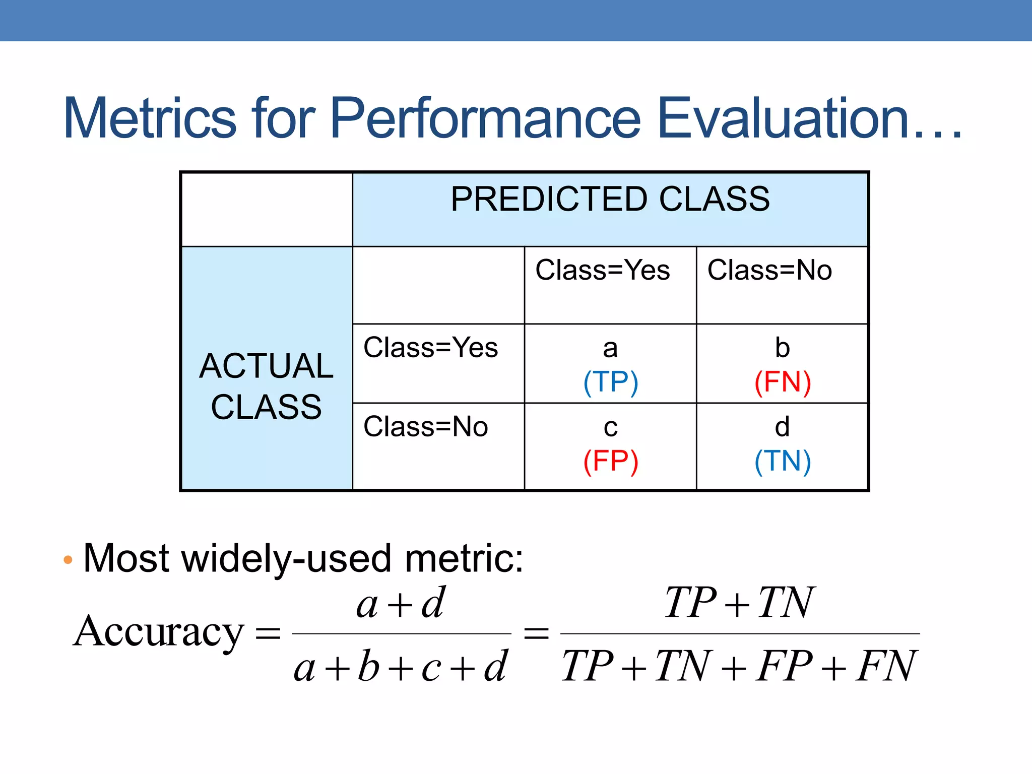
Accuracy = (a + d)/N
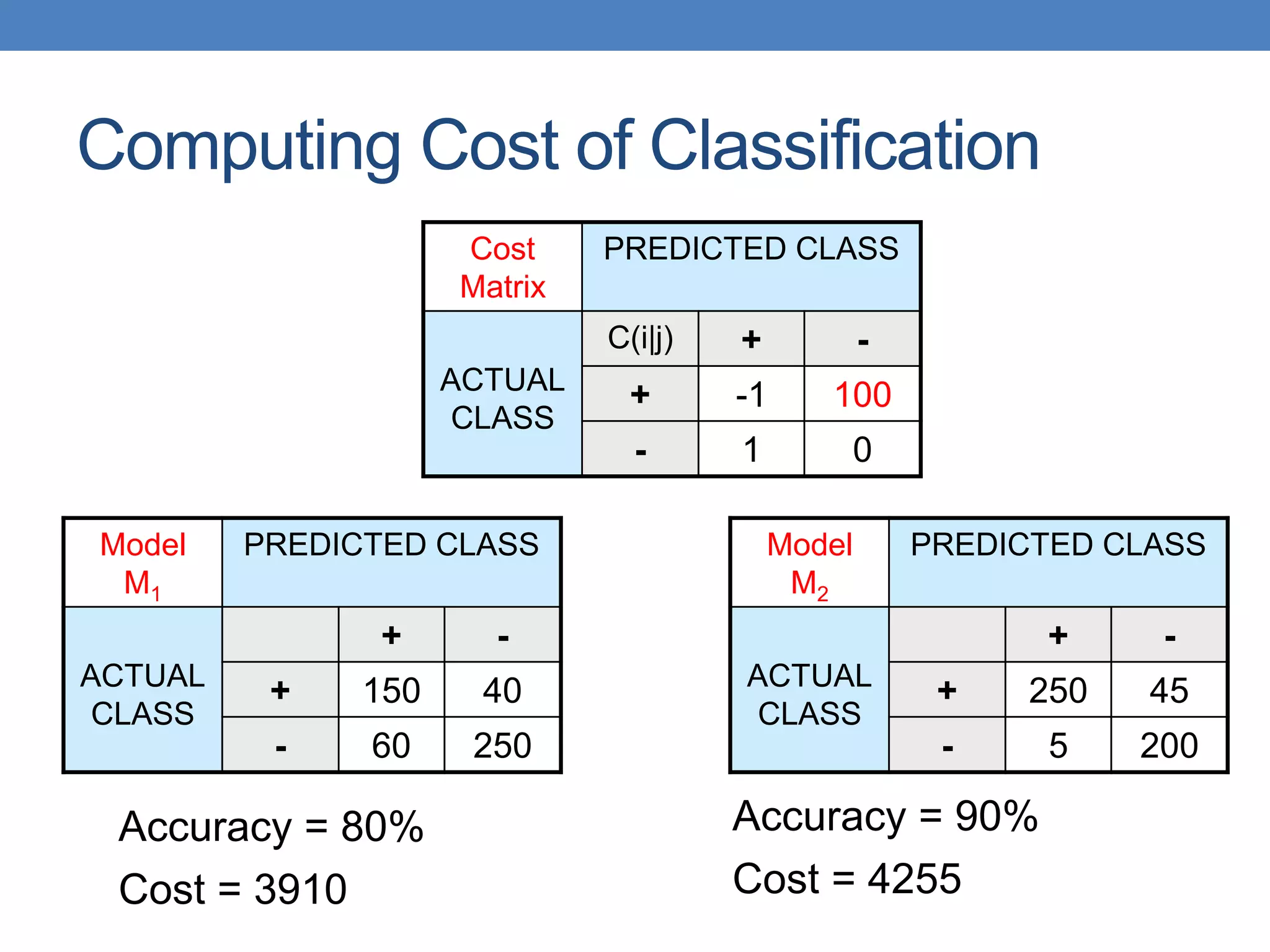
Cost = p (a + d) + q (b + c)
= p (a + d) + q (N – a – d)
= q N – (q – p)(a + d)
= N [q – (q-p) Accuracy]
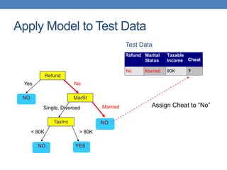
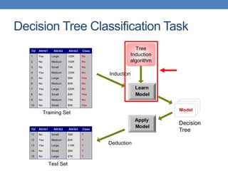
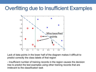
Accuracy is proportional to cost if
1. C(Yes|No)=C(No|Yes) = q
2. C(Yes|Yes)=C(No|No) = p](https://image.slidesharecdn.com/datamininglecture10a-230924165908-aceffac8/85/Data-Mining-Lecture_10-a-pptx-73-320.jpg)


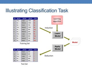
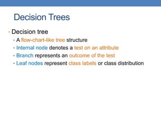
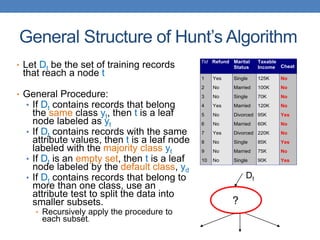
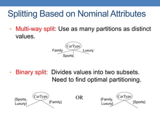
![Cost vs Accuracy
Count PREDICTED CLASS
ACTUAL
CLASS
Class=Yes Class=No
Class=Yes a b
Class=No c d
Cost PREDICTED CLASS
ACTUAL
CLASS
Class=Yes Class=No
Class=Yes p q
Class=No q p
N = a + b + c + d
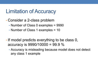
Accuracy = (a + d)/N
Cost = p (a + d) + q (b + c)
= p (a + d) + q (N – a – d)
= q N – (q – p)(a + d)
= N [q – (q-p) Accuracy]
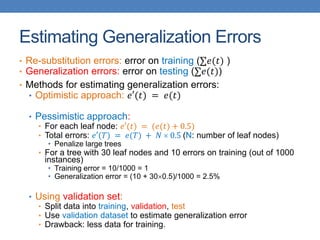
Accuracy is proportional to cost if
1. C(Yes|No)=C(No|Yes) = q
2. C(Yes|Yes)=C(No|No) = p](https://image.slidesharecdn.com/datamininglecture10a-230924165908-aceffac8/75/Data-Mining-Lecture_10-a-pptx-73-2048.jpg)


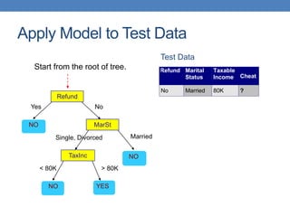
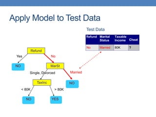
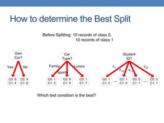
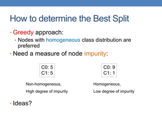
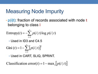
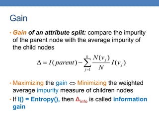
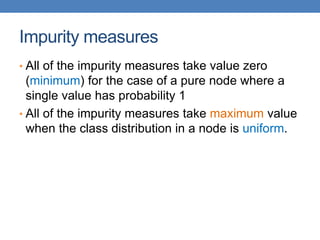
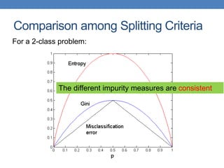
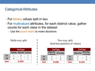
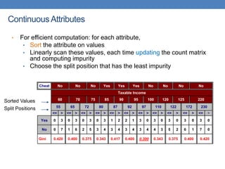
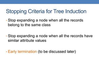
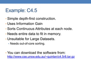
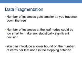
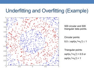
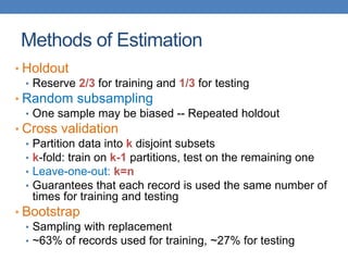
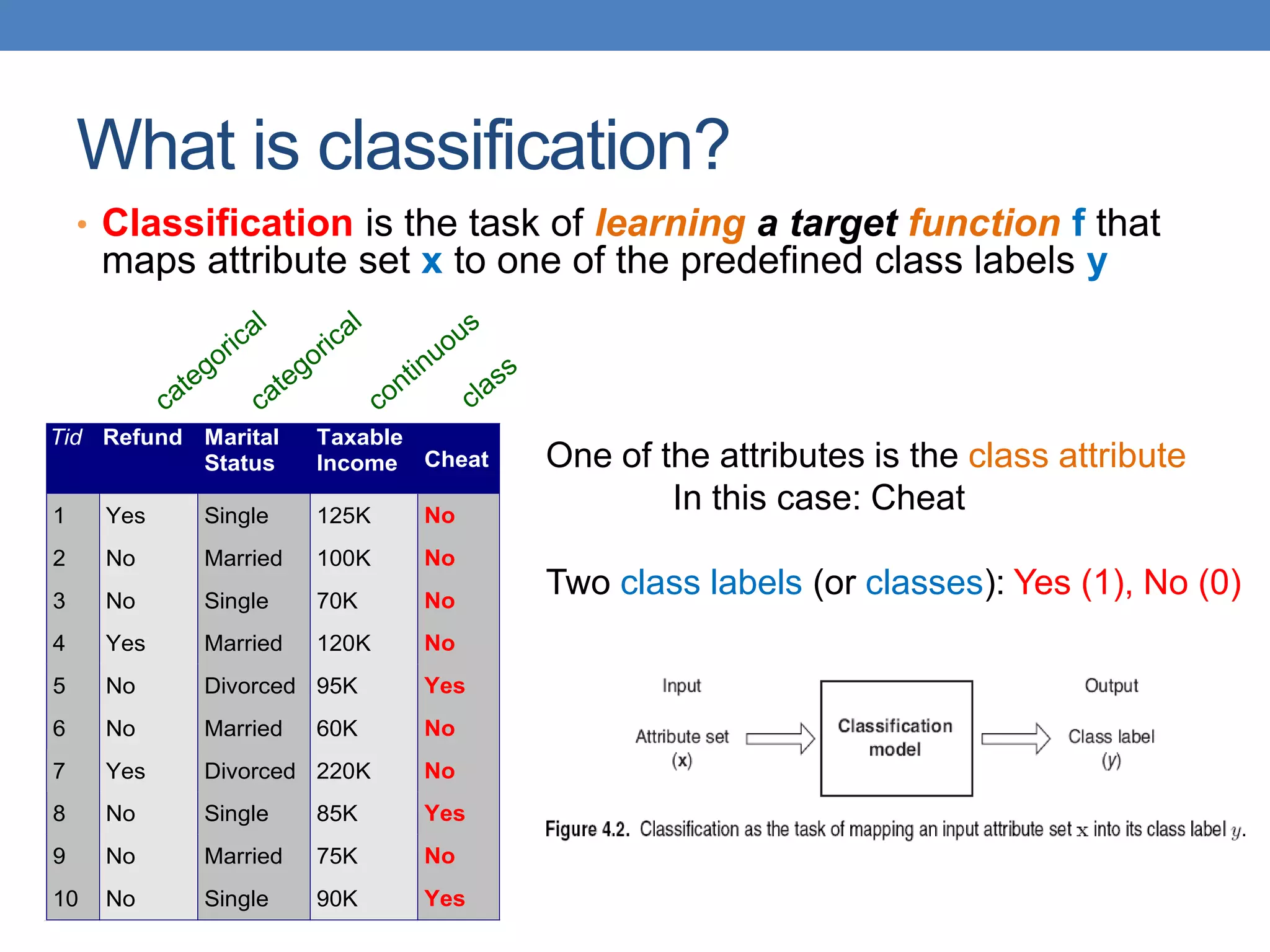
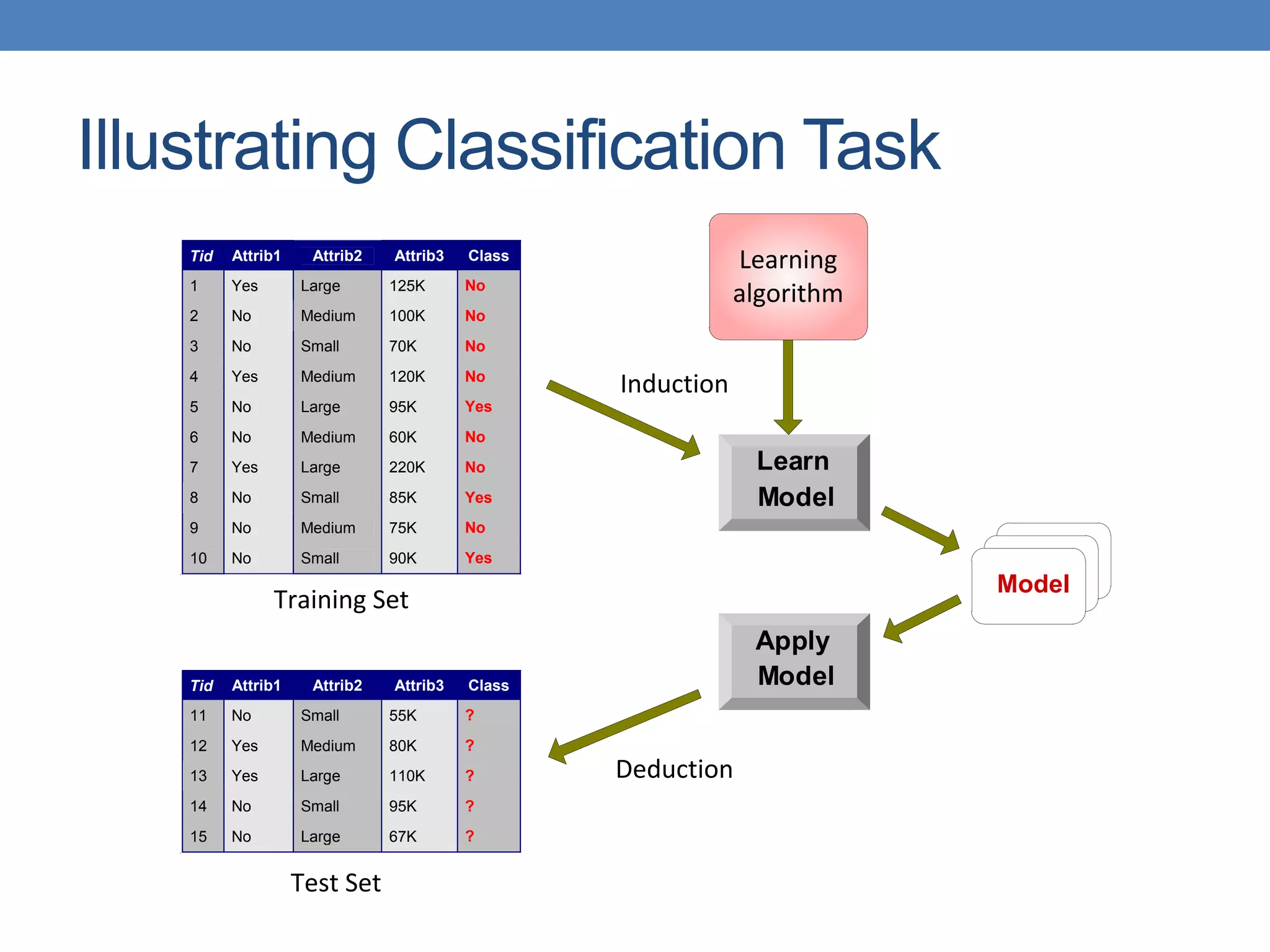
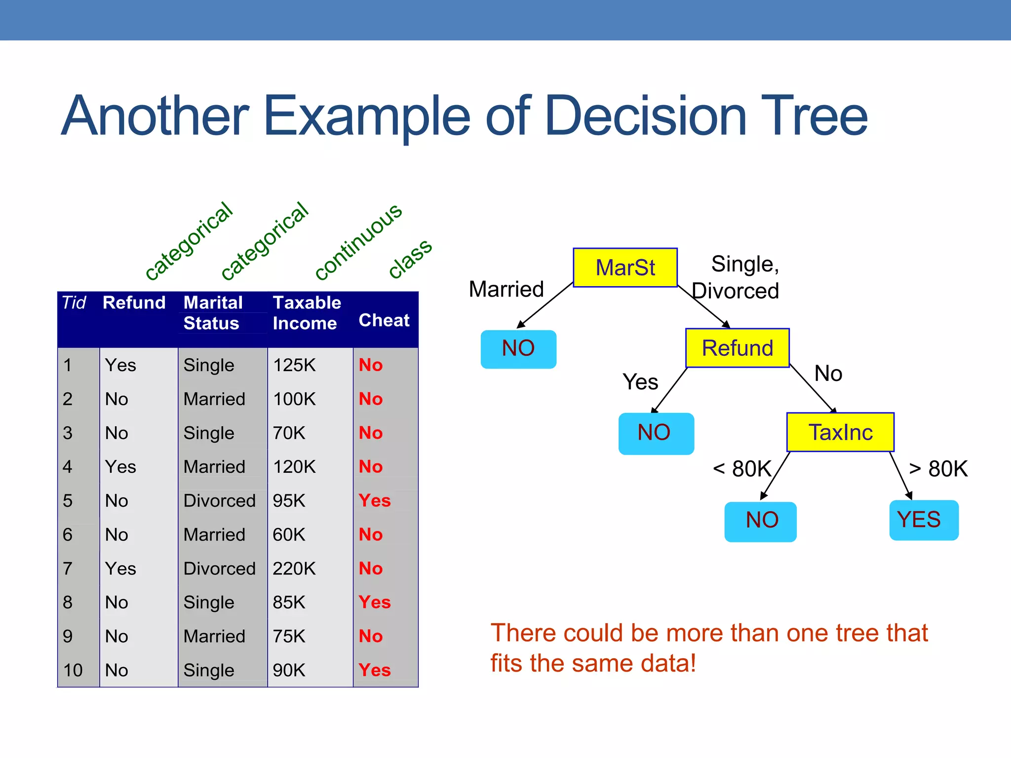
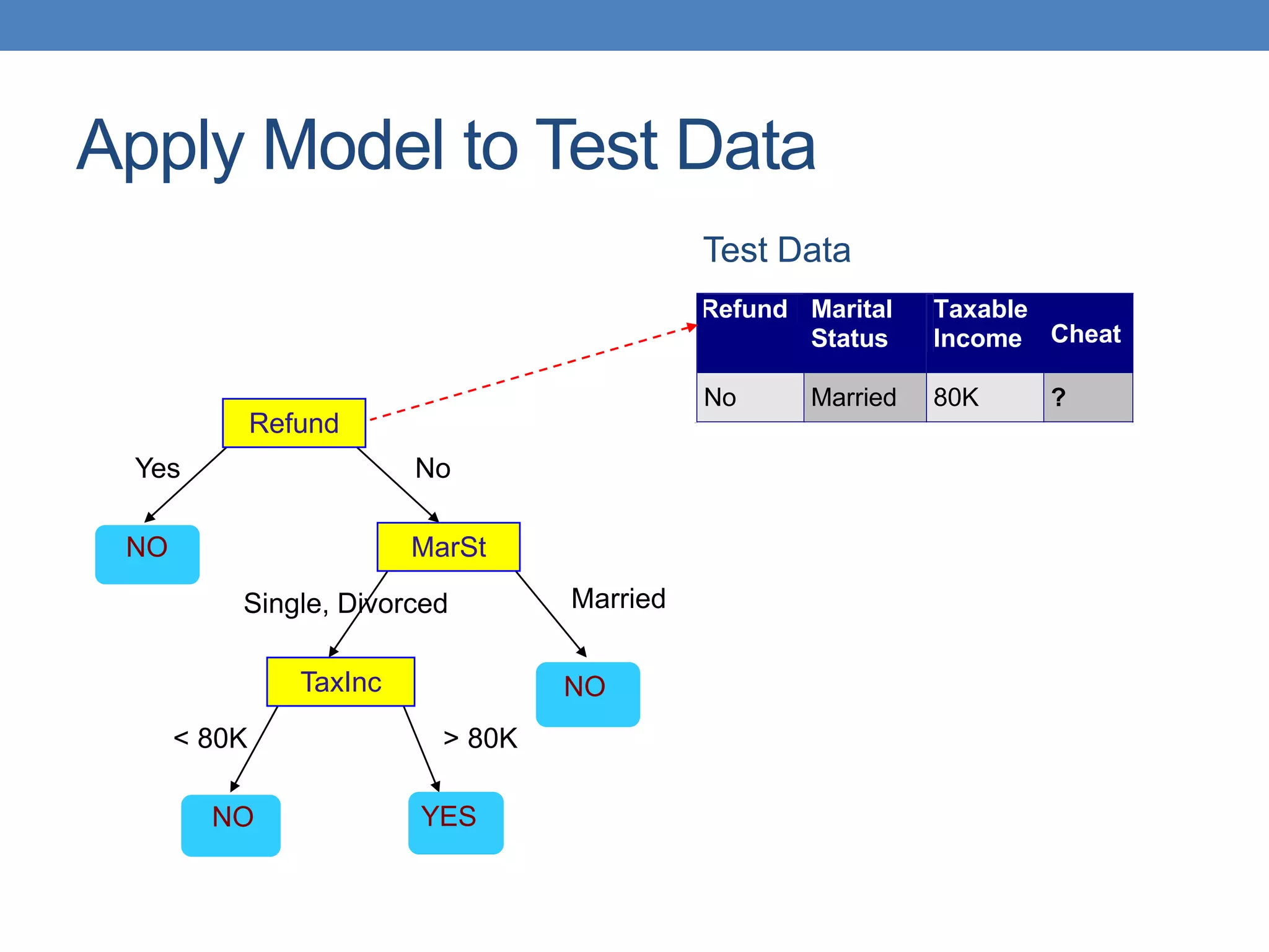
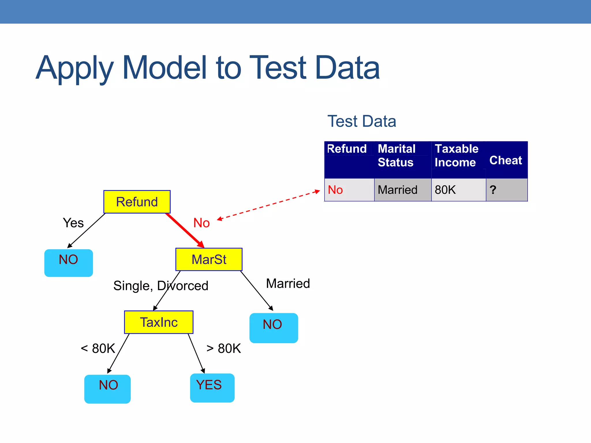
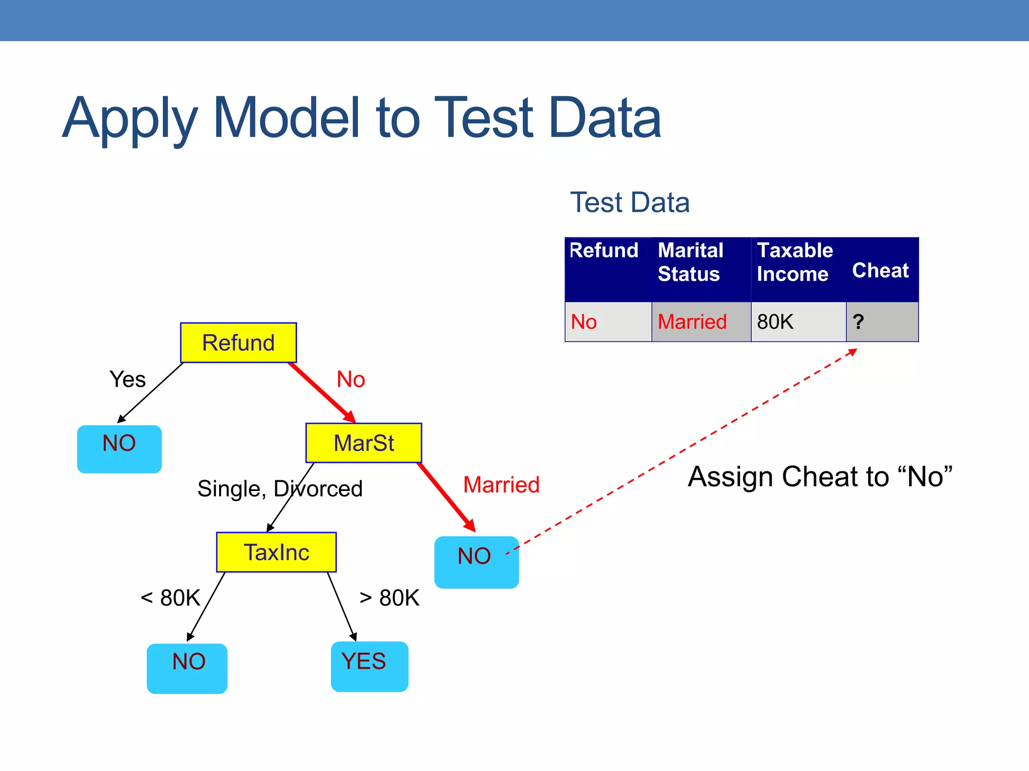
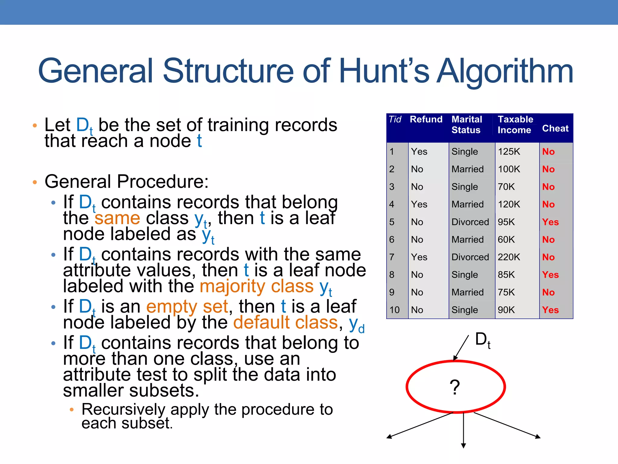
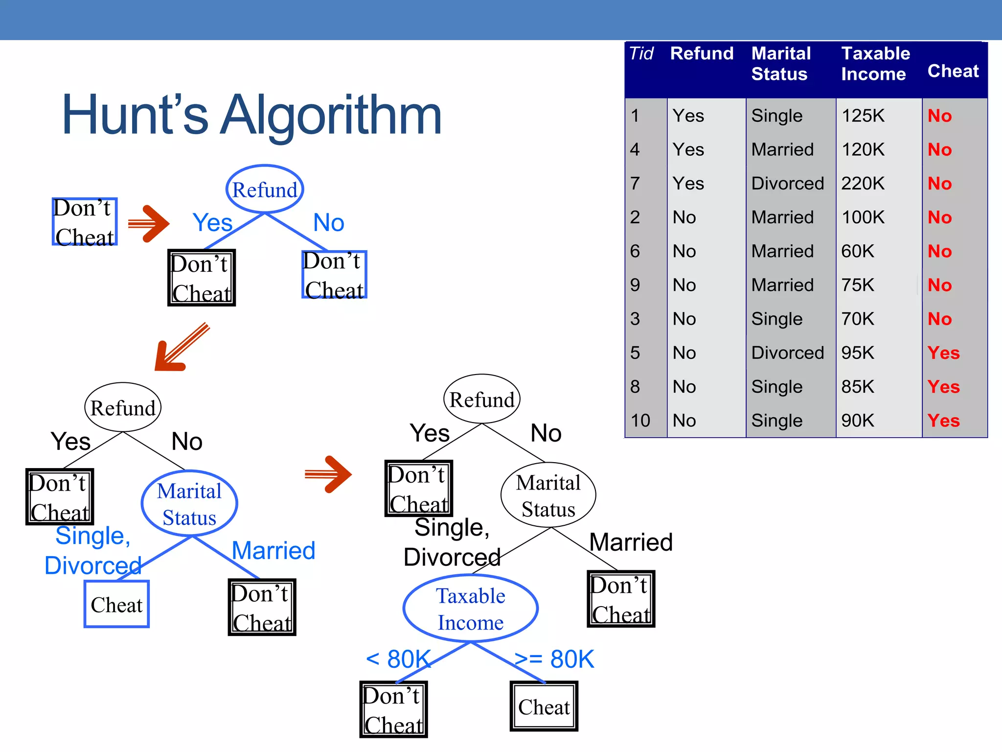
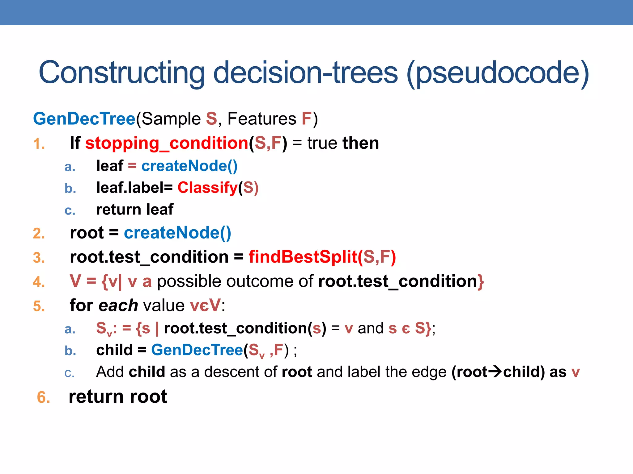
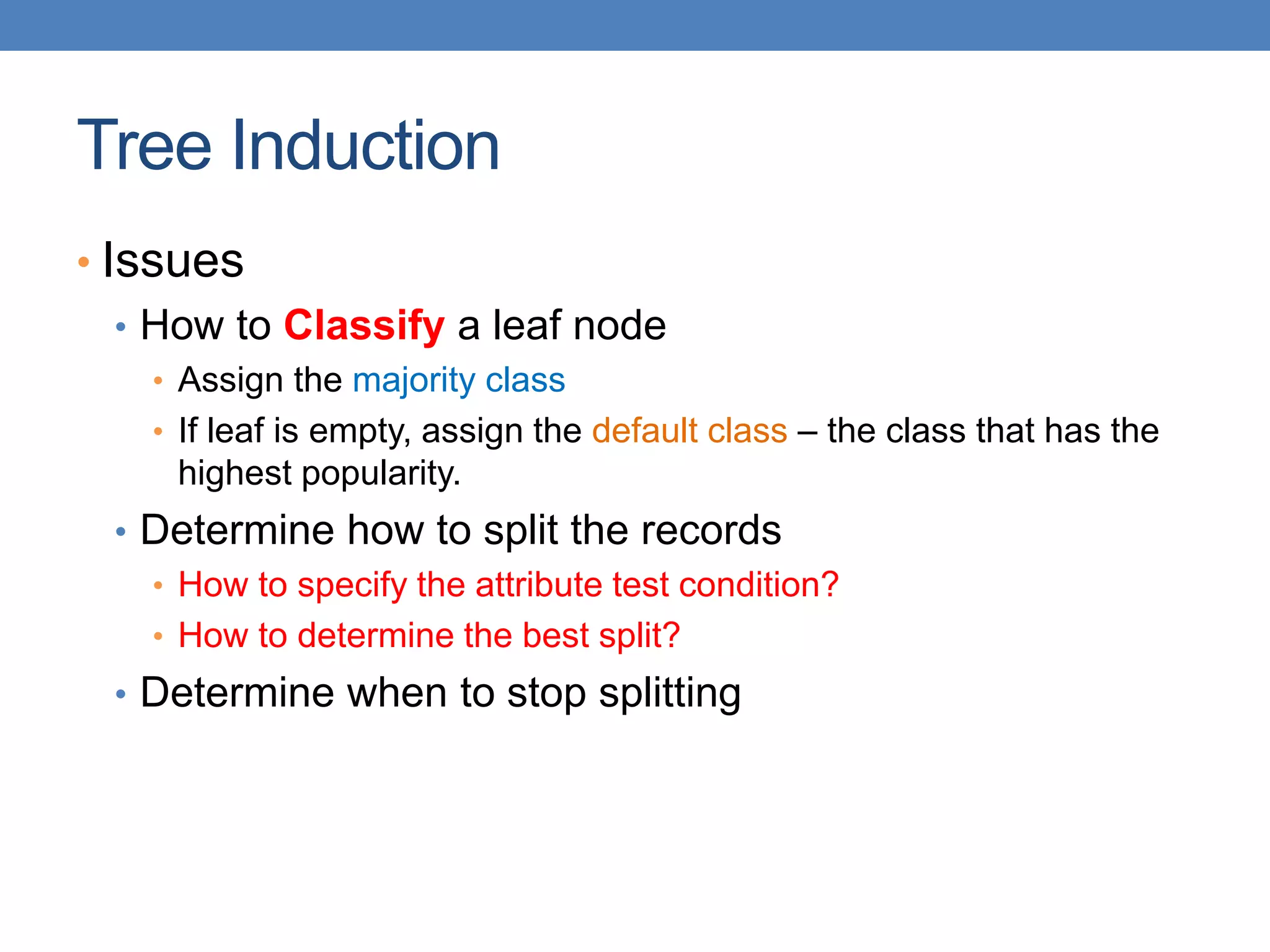
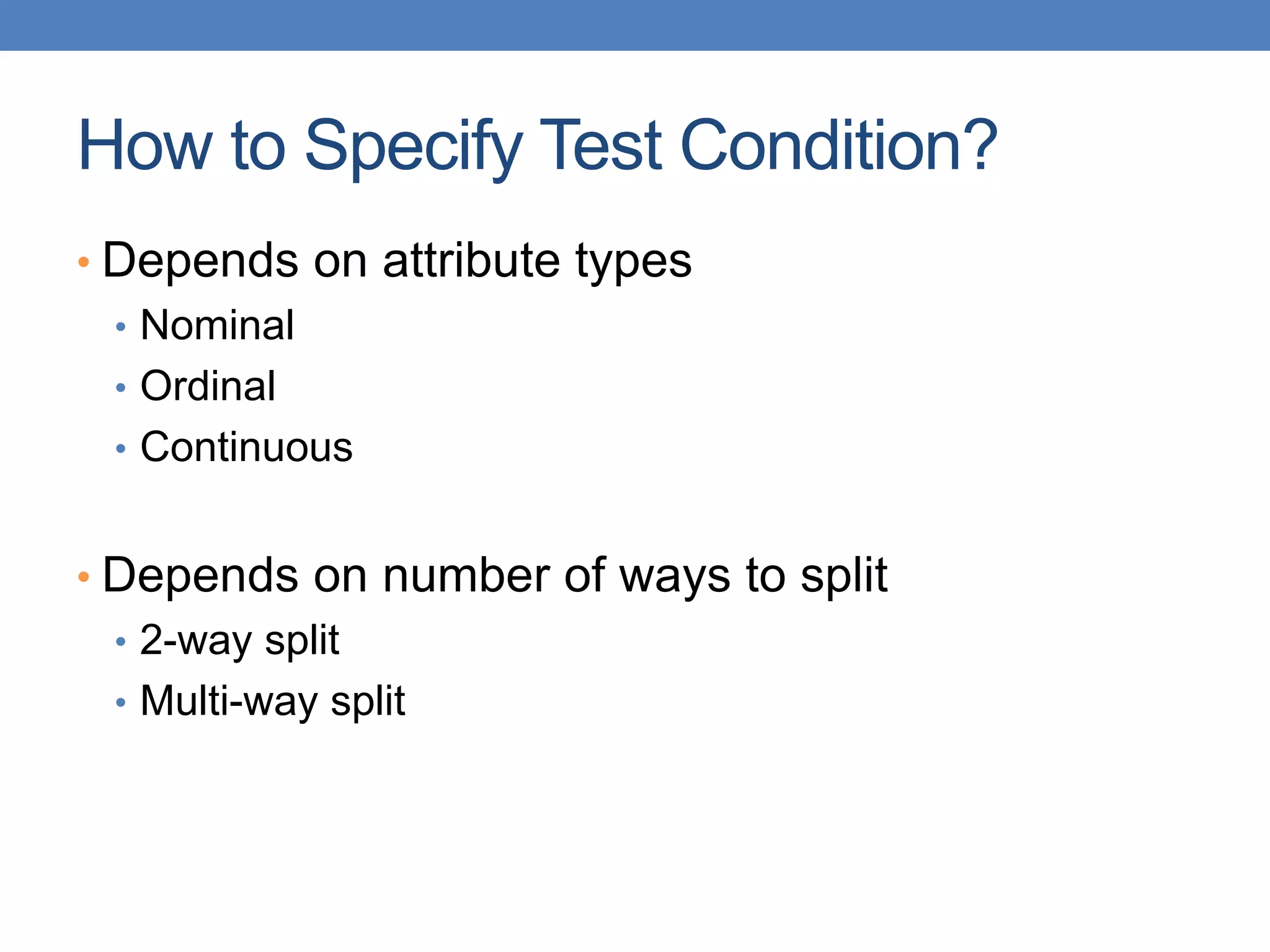
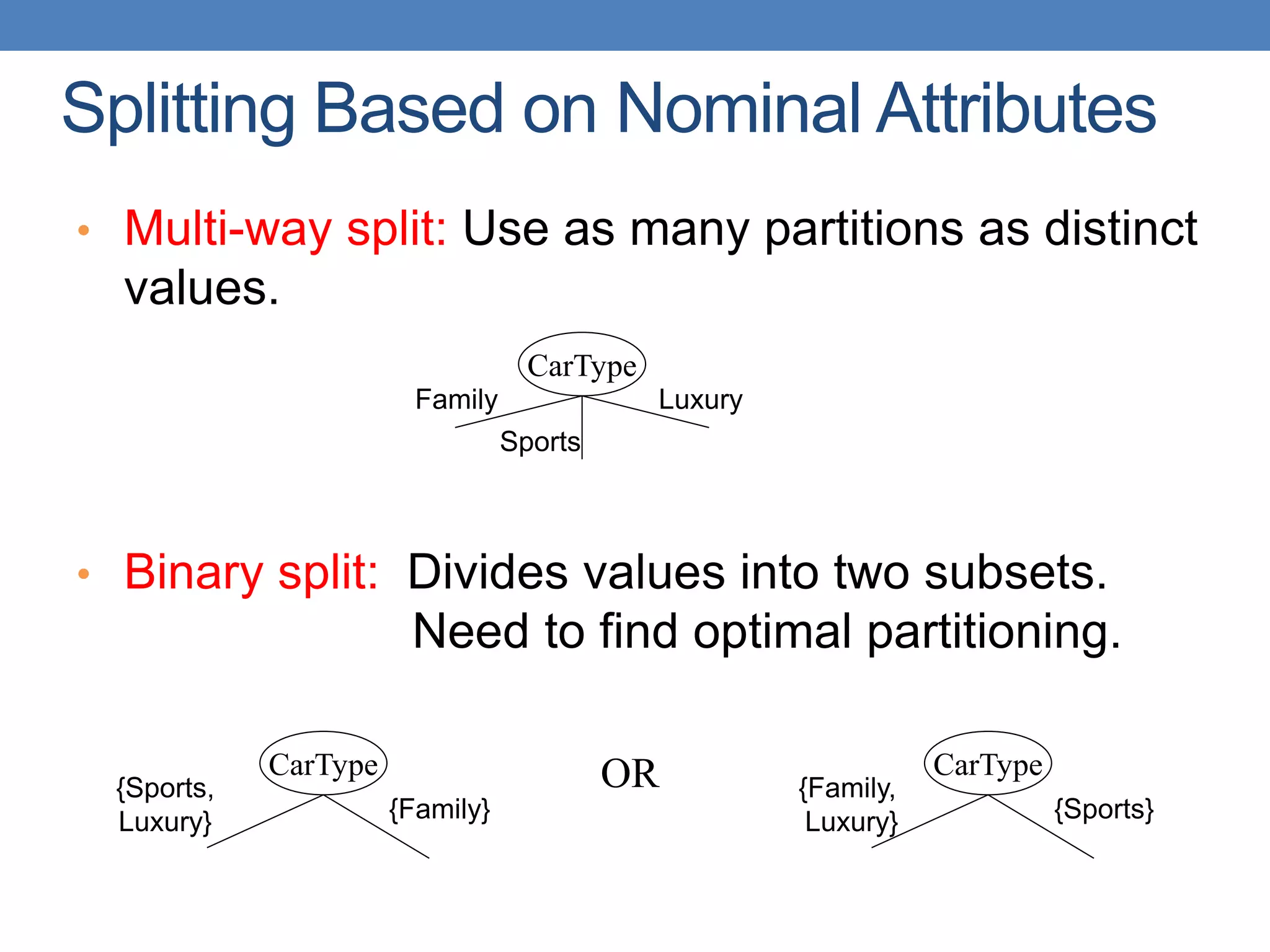
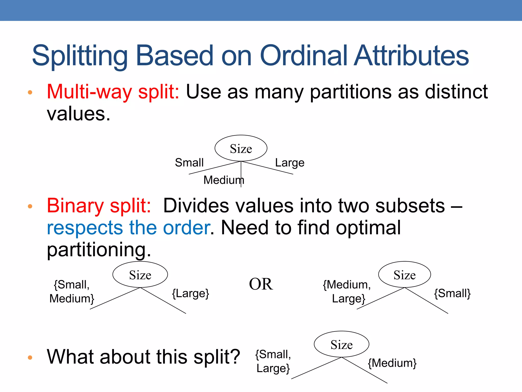
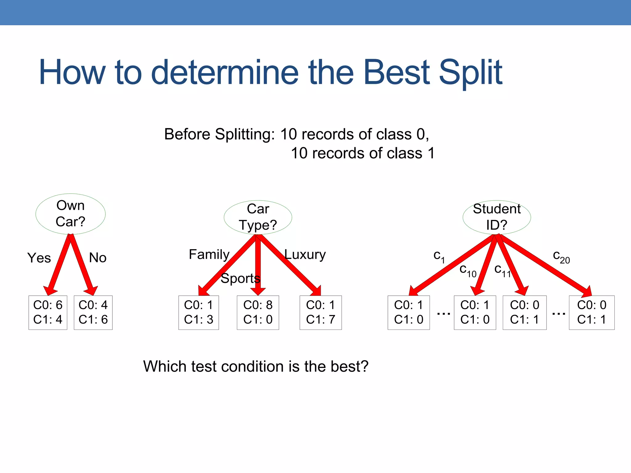
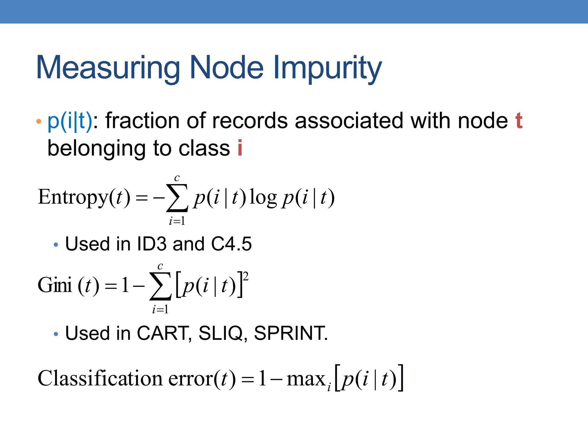
The document covers classification concepts in data mining, specifically focusing on decision trees used for predicting tax evasion based on attributes like marital status and taxable income. It discusses the process of building classification models, evaluating their effectiveness using confusion matrices, and outlines various classification techniques. Additionally, it delves into decision tree construction, including attribute selection and impurity measurements, emphasizing methods such as ID3, C4.5, and CART.


