Data Wrangling
Validating Data,Manipulating Categorical
Variables, Dealing with Missing Data, Slicing and
Dicing: Filtering and Selecting Data, Concatenating
and Transforming, Aggregating Data at Any Leve
2.
• Data Wranglingis the process of gathering, collecting, and transforming Raw data into
another format for better understanding, decision-making, accessing, and analysis in
less time.
• Data Wrangling is also known as Data Munging
• Data wrangling is the process of standardizing disorganized or incomplete raw data.
• make data more accessible and suitable for analytics.
• targeting a field, row, or column in a dataset and implementing an action like joining,
parsing, cleaning, consolidating, or filtering to produce the required output.
• After wrangling, you can use the data to process it further for business intelligence (BI),
reporting, or improving business processes.
• process ensures the data is ready for automation and further analysis.
• professionals spend almost 73% of their time wrangling data
• It helps business users make concrete, timely decisions by cleaning and structuring raw
data into the required format.
• Data wrangling is becoming a common practice among top organizations as the data
becomes more unstructured and diverse.
• it is an iterative process in which you must perform the five steps recurrently to get your
desired results
3.
Steps to PerformData Wrangling
Understanding Data
• The first step is to understand the data in great depth.
• Before applying procedures to clean it, you must have
a clear idea of what the data is about.
• This will help you find the best approach for
productive analytic explorations.
• For exa, if you have a customer dataset and learn that
most of your customers are from one part of the
country, you’ll keep that in mind before progressing.
4.
Structuring
• Mostly wehave raw data in a disorganized
manner.
• There won’t be any structure to it.
• In the second step, you have to restructure
the data type for easy accessibility, which
might mean splitting one column or row into
two or vice versa – whatever is needed for
better analysis.
5.
Cleansing
• Almost everydataset includes some outliers that can skew
the outcomes of the analysis.
• You’ll have to clean the data for optimum results.
• In the third step, you have to clean the data exhaustively for
superior analysis.
• You’ll have to change null values, remove duplicates and
special characters, and standardize the formatting to
improve the consistency of the data.
• For example, you may replace the many different ways that
a state is recorded (such as GUJ, GJ, and GUJARAT) with a
single standard format.
6.
Enriching
• After thethird step, you must enrich your
data, which means taking stock of what’s in
the dataset and strategizing how to improve it.
For example, a car insurance company might
want to know crime rates in the
neighborhoods of its users to estimate risk
better.
7.
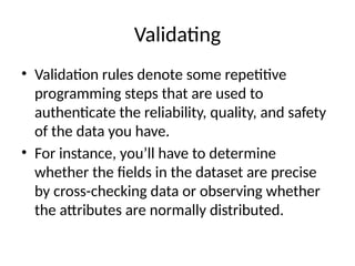
Validating
• Validation rulesdenote some repetitive
programming steps that are used to
authenticate the reliability, quality, and safety
of the data you have.
• For instance, you’ll have to determine
whether the fields in the dataset are precise
by cross-checking data or observing whether
the attributes are normally distributed.
8.
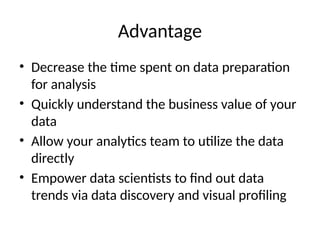
Advantage
• Decrease thetime spent on data preparation
for analysis
• Quickly understand the business value of your
data
• Allow your analytics team to utilize the data
directly
• Empower data scientists to find out data
trends via data discovery and visual profiling
9.
Data wrangling inPython
• deals with the below functionalities:
• Data exploration: In this process, the data is studied, analyzed, and understood by
visualizing representations of data.
• Dealing with missing values: Most of the datasets having a vast amount of data
contain missing values of NaN, they are needed to be taken care of by replacing
them with mean, mode, the most frequent value of the column, or simply by
dropping the row having a NaN value.
• Reshaping data: In this process, data is manipulated according to the requirements,
where new data can be added or pre-existing data can be modified.
• Filtering data: Some times datasets are comprised of unwanted rows or columns
which are required to be removed or filtered
• Other: After dealing with the raw dataset with the above functionalities we get an
efficient dataset as per our requirements and then it can be used for a required
purpose like data analyzing, machine learning, data visualization, model training etc.
10.
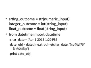
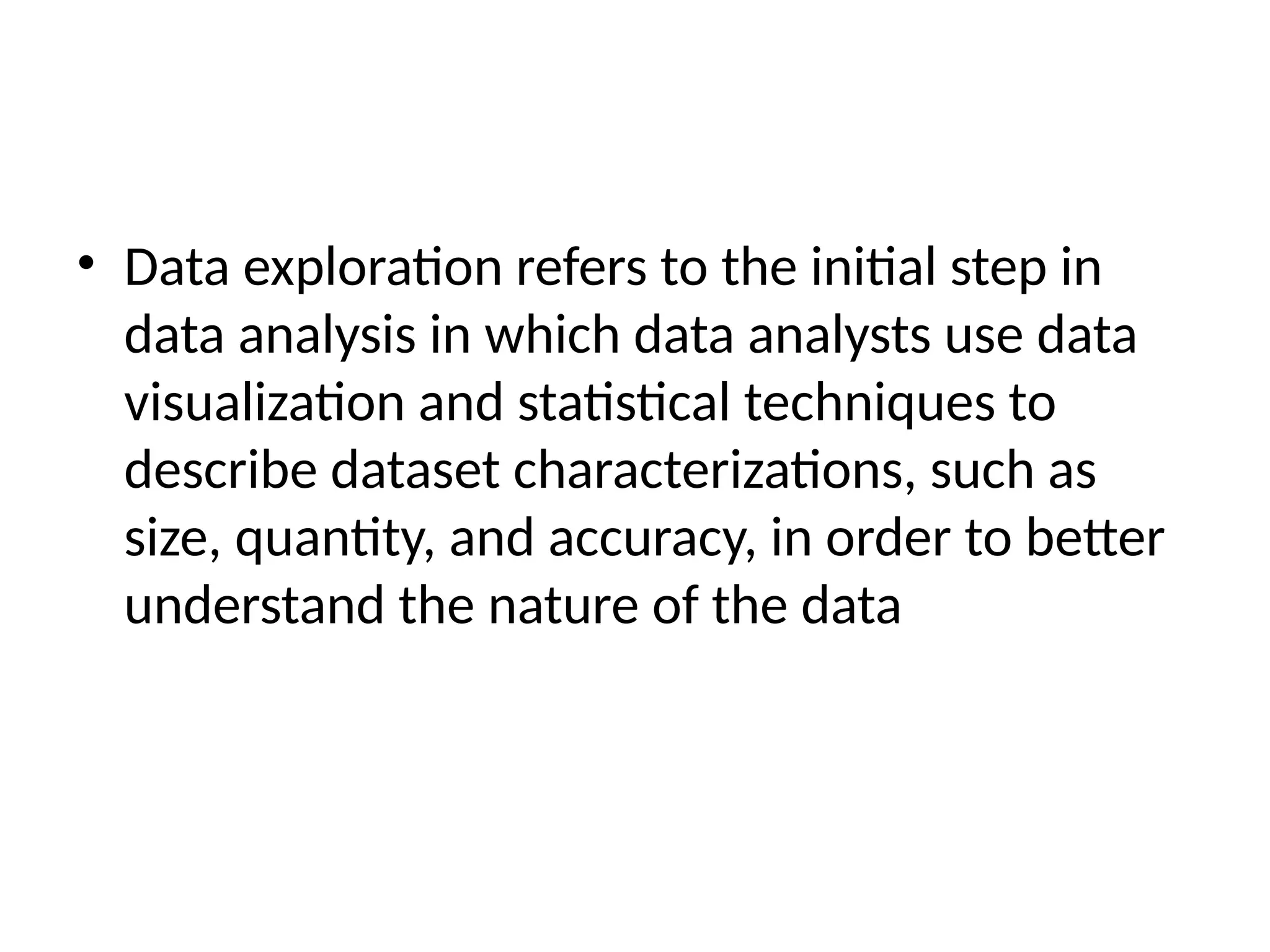
• Data explorationrefers to the initial step in
data analysis in which data analysts use data
visualization and statistical techniques to
describe dataset characterizations, such as
size, quantity, and accuracy, in order to better
understand the nature of the data
• Distribution ofAge
import matplotlib.pyplot as plt
import pandas as pd
df=pd.read_excel("E:/First.xlsx", "Sheet1")
fig=plt.figure()
ax = fig.add_subplot(1,1,1)
ax.hist(df['Age'],bins = 5)
plt.title('Age distribution')
plt.xlabel('Age')
plt.ylabel('#Employee')
plt.show()
16.
• Relationship betweenage and sales
plt.scatter(df['Age'],df['Sales'])
plt.title('Sales and Age distribution')
plt.xlabel('Age')
plt.ylabel('Sales')
plt.show()
df=pd.read_csv("E:AcademicEVENHPP.csv")
plt.scatter(df['YearBuilt'],df['SalePrice'])
plt.show()
import seaborn as sns
sns.boxplot(df['Age'])
17.
• frequency tables
importpandas as pd
df=pd.read_csv("E:AcademicEVENHPP.csv")
test= df.groupby(['MSSubClass','OverallCond'])
test.size()
• #Create Sample dataframe
import numpy as np
import pandas as pd
from random import sample
df=pd.read_csv("E:AcademicEVENstudy_performance.csv")
rindex = np.array(sample(range(len(df)), 5))
dfr = df.loc[rindex]
print(dfr)
18.
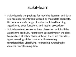
Scikit-learn
• Scikit-learn isthe package for machine learning and data
science experimentation favored by most data scientists.
It contains a wide range of well-established learning
algorithms, error functions, and testing procedures.
• Scikit-learn features some base classes on which all the
algorithms are built. Apart from BaseEstimator, the class
from which all other classes inherit, there are four class
types covering all the basic machinelearning
functionalities: Classifying, Regressing, Grouping by
clusters, Transforming data
19.
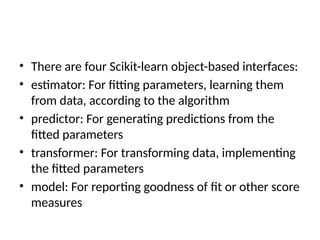
• There arefour Scikit-learn object-based interfaces:
• estimator: For fitting parameters, learning them
from data, according to the algorithm
• predictor: For generating predictions from the
fitted parameters
• transformer: For transforming data, implementing
the fitted parameters
• model: For reporting goodness of fit or other score
measures
20.
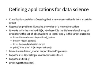
Defining applications fordata science
• Classification problem: Guessing that a new observation is from a certain
group
• Regression problem: Guessing the value of a new observation
• It works with the method fit(X, y) where X is the bidimensional array of
predictors (the set of observations to learn) and y is the target outcome
– from sklearn.datasets import load_boston
– boston = load_boston()
– X, y = boston.data,boston.target
– print("X:%s y:%s" % (X.shape, y.shape))
• from sklearn.linear_model import LinearRegression
• hypothesis = LinearRegression(normalize=True)
• hypothesis.fit(X, y)
• print(hypothesis.coef)_
21.
• A hypothesisis a way to describe a learning
algorithm trained with data. The hypothesis
defines a possible representation of y given X that
you test for validity.
– import numpy as np
– new_observation = np.array([1, 0, 1, 0, 0.5, 7, 59, 6, 3, 200, 20, 350,
4], dtype=float).reshape(1, -1)
– print(hypothesis.predict(new_observation))
– hypothesis.score(X, y)
hashing trick
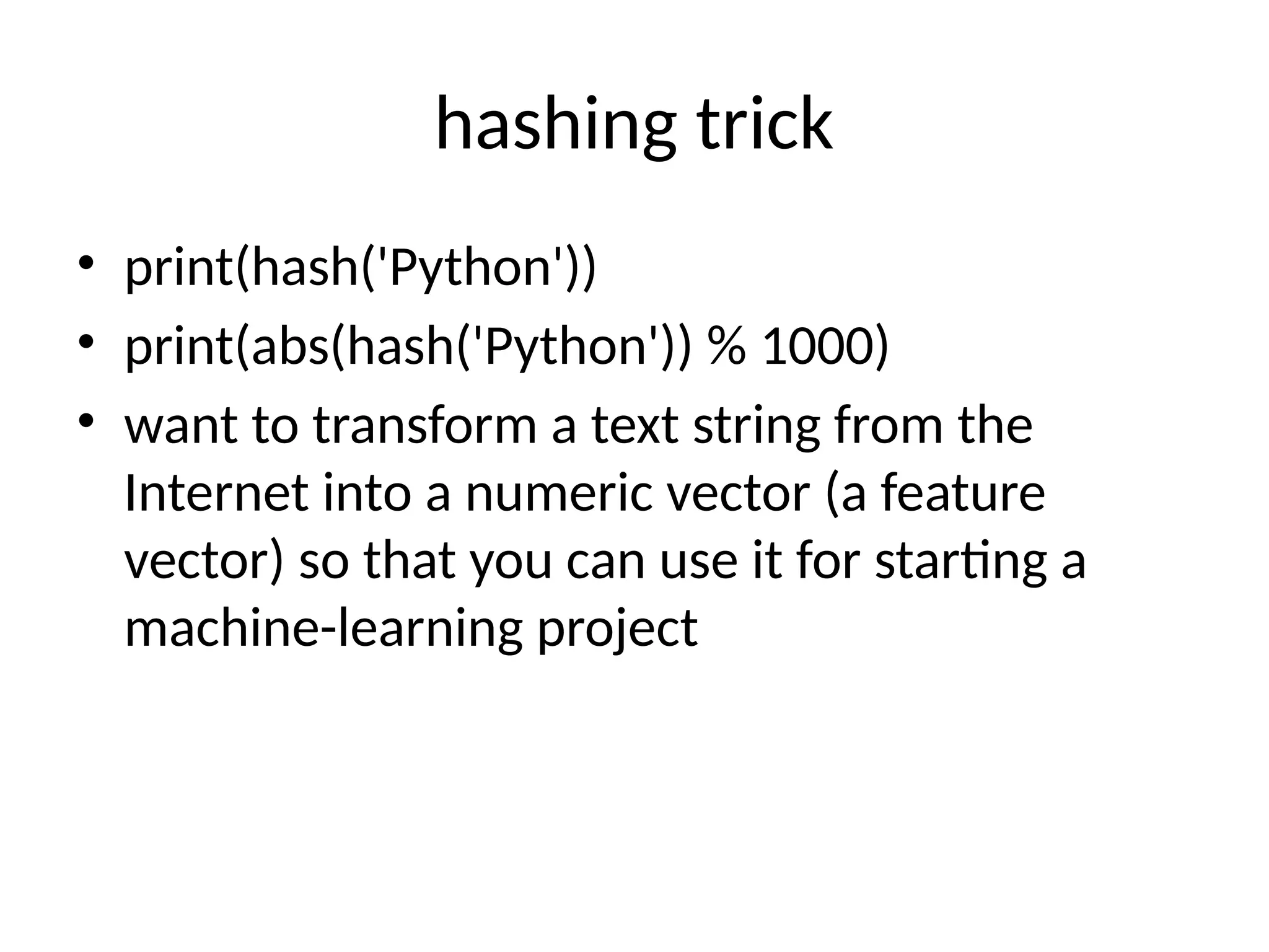
• print(hash('Python'))
•print(abs(hash('Python')) % 1000)
• want to transform a text string from the
Internet into a numeric vector (a feature
vector) so that you can use it for starting a
machine-learning project
24.
one-hot encoding
• fromsklearn.feature_extraction.text import *
oh_enconder = CountVectorizer() oh_enconded =
oh_enconder.fit_transform([ 'Python for data
science','Python for machine learning'])
• print(oh_enconder.vocabulary_)
25.
• Ex
Employee_Id GenderRemarks
45Male Nice
78Female Good
56Female Great
12Male Great
7Female Nice
68Female Great
23Male Good
45Female Nice
89Male Great
75Female Nice
47Female Good
62Male Nice
#1)
import pandas as pd
import numpy as np
from sklearn.preprocessing import
OneHotEncoder
data = pd.read_csv('Employee_data.csv')
data['Gender'] =
data['Gender'].astype('category')
data['Remarks'] =
data['Remarks'].astype('category')
data['Gen_new'] = data['Gender'].cat.codes
data['Rem_new'] = data['Remarks'].cat.codes
enc = OneHotEncoder()
enc_data = pd.DataFrame(enc.fit_transform(
data[['Gen_new', 'Rem_new']]).toarray())
New_df = data.join(enc_data)
print(New_df)
2)
one_hot_encoded_data = pd.get_dummies(data, columns = ['Remarks', 'Gender'])
print(one_hot_encoded_data)
Timing and Performance
•%timeit: Calculates the best performance time for an instruction.
• %%timeit: Calculates the best time performance for all the instructions in a cell,
apart from the one placed on the same cell line as the cell magic
• %timeit l = [k for k in range(10**6)]
%%timeit
l = list()
for k in range(10**6):
l.append(k)
28.
memory profiler
• pipinstall memory_profiler
• %load_ext memory_profiler
• %memit
• import sklearn.feature_extraction.text as txthtrick =
txt.HashingVectorizer(n_features=20,binary=True,no
rm=None)texts = ['Python for data science','Python
for machine learning']hashing =
htrick.transform(texts)%memit dense_hashing =
hashing.toarray()
29.
• %%writefile example_code.py
•def comparison_test(text):
import sklearn.feature_extraction.text as txt
htrick = txt.HashingVectorizer(n_features=20, binary=True,
norm=None)
oh_enconder = txt.CountVectorizer()
oh_enconded = oh_enconder.fit_transform(text)
hashing = htrick.transform(text)
return oh_enconded, hashing
from example_code import comparison_test
text = ['Python for data science', 'Python for machine learning']
%mprun -f comparison_test comparison_test(text)


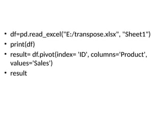
![• df=pd.read_excel("E:/transpose.xlsx", "Sheet1")
• print df.sort(['Product','Sales'], ascending=[True,
False])](https://image.slidesharecdn.com/datawrangling-250815070344-381f8adf/85/Data-Wrangling-pptx-use-to-in-pandas-in-data-14-320.jpg)
![• Distribution of Age
import matplotlib.pyplot as plt
import pandas as pd
df=pd.read_excel("E:/First.xlsx", "Sheet1")
fig=plt.figure()
ax = fig.add_subplot(1,1,1)
ax.hist(df['Age'],bins = 5)
plt.title('Age distribution')
plt.xlabel('Age')
plt.ylabel('#Employee')
plt.show()](https://image.slidesharecdn.com/datawrangling-250815070344-381f8adf/85/Data-Wrangling-pptx-use-to-in-pandas-in-data-15-320.jpg)
![• Relationship between age and sales
plt.scatter(df['Age'],df['Sales'])
plt.title('Sales and Age distribution')
plt.xlabel('Age')
plt.ylabel('Sales')
plt.show()
df=pd.read_csv("E:AcademicEVENHPP.csv")
plt.scatter(df['YearBuilt'],df['SalePrice'])
plt.show()
import seaborn as sns
sns.boxplot(df['Age'])](https://image.slidesharecdn.com/datawrangling-250815070344-381f8adf/85/Data-Wrangling-pptx-use-to-in-pandas-in-data-16-320.jpg)
![• frequency tables
import pandas as pd
df=pd.read_csv("E:AcademicEVENHPP.csv")
test= df.groupby(['MSSubClass','OverallCond'])
test.size()
• #Create Sample dataframe
import numpy as np
import pandas as pd
from random import sample
df=pd.read_csv("E:AcademicEVENstudy_performance.csv")
rindex = np.array(sample(range(len(df)), 5))
dfr = df.loc[rindex]
print(dfr)](https://image.slidesharecdn.com/datawrangling-250815070344-381f8adf/85/Data-Wrangling-pptx-use-to-in-pandas-in-data-17-320.jpg)
![• A hypothesis is a way to describe a learning
algorithm trained with data. The hypothesis
defines a possible representation of y given X that
you test for validity.
– import numpy as np
– new_observation = np.array([1, 0, 1, 0, 0.5, 7, 59, 6, 3, 200, 20, 350,
4], dtype=float).reshape(1, -1)
– print(hypothesis.predict(new_observation))
– hypothesis.score(X, y)](https://image.slidesharecdn.com/datawrangling-250815070344-381f8adf/85/Data-Wrangling-pptx-use-to-in-pandas-in-data-21-320.jpg)

![one-hot encoding
• from sklearn.feature_extraction.text import *
oh_enconder = CountVectorizer() oh_enconded =
oh_enconder.fit_transform([ 'Python for data
science','Python for machine learning'])
• print(oh_enconder.vocabulary_)](https://image.slidesharecdn.com/datawrangling-250815070344-381f8adf/85/Data-Wrangling-pptx-use-to-in-pandas-in-data-24-320.jpg)
![• Ex
Employee_Id Gender Remarks
45Male Nice
78Female Good
56Female Great
12Male Great
7Female Nice
68Female Great
23Male Good
45Female Nice
89Male Great
75Female Nice
47Female Good
62Male Nice
#1)
import pandas as pd
import numpy as np
from sklearn.preprocessing import
OneHotEncoder
data = pd.read_csv('Employee_data.csv')
data['Gender'] =
data['Gender'].astype('category')
data['Remarks'] =
data['Remarks'].astype('category')
data['Gen_new'] = data['Gender'].cat.codes
data['Rem_new'] = data['Remarks'].cat.codes
enc = OneHotEncoder()
enc_data = pd.DataFrame(enc.fit_transform(
data[['Gen_new', 'Rem_new']]).toarray())
New_df = data.join(enc_data)
print(New_df)
2)
one_hot_encoded_data = pd.get_dummies(data, columns = ['Remarks', 'Gender'])
print(one_hot_encoded_data)](https://image.slidesharecdn.com/datawrangling-250815070344-381f8adf/85/Data-Wrangling-pptx-use-to-in-pandas-in-data-25-320.jpg)
![• from scipy.sparse import csc_matrix print
csc_matrix([1, 0, 0, 0, 0, 1, 0, 0, 0, 0, 0, 0, 0, 0,
0, 0, 1, 0, 1, 0])
• (0, 0) 1
• (0, 5) 1
• (0, 16) 1
• (0, 18) 1](https://image.slidesharecdn.com/datawrangling-250815070344-381f8adf/85/Data-Wrangling-pptx-use-to-in-pandas-in-data-26-320.jpg)
![Timing and Performance
• %timeit: Calculates the best performance time for an instruction.
• %%timeit: Calculates the best time performance for all the instructions in a cell,
apart from the one placed on the same cell line as the cell magic
• %timeit l = [k for k in range(10**6)]
%%timeit
l = list()
for k in range(10**6):
l.append(k)](https://image.slidesharecdn.com/datawrangling-250815070344-381f8adf/85/Data-Wrangling-pptx-use-to-in-pandas-in-data-27-320.jpg)
![memory profiler
• pip install memory_profiler
• %load_ext memory_profiler
• %memit
• import sklearn.feature_extraction.text as txthtrick =
txt.HashingVectorizer(n_features=20,binary=True,no
rm=None)texts = ['Python for data science','Python
for machine learning']hashing =
htrick.transform(texts)%memit dense_hashing =
hashing.toarray()](https://image.slidesharecdn.com/datawrangling-250815070344-381f8adf/85/Data-Wrangling-pptx-use-to-in-pandas-in-data-28-320.jpg)
![• %%writefile example_code.py
• def comparison_test(text):
import sklearn.feature_extraction.text as txt
htrick = txt.HashingVectorizer(n_features=20, binary=True,
norm=None)
oh_enconder = txt.CountVectorizer()
oh_enconded = oh_enconder.fit_transform(text)
hashing = htrick.transform(text)
return oh_enconded, hashing
from example_code import comparison_test
text = ['Python for data science', 'Python for machine learning']
%mprun -f comparison_test comparison_test(text)](https://image.slidesharecdn.com/datawrangling-250815070344-381f8adf/85/Data-Wrangling-pptx-use-to-in-pandas-in-data-29-320.jpg)


![• df=pd.read_excel("E:/transpose.xlsx", "Sheet1")
• print df.sort(['Product','Sales'], ascending=[True,
False])](https://image.slidesharecdn.com/datawrangling-250815070344-381f8adf/75/Data-Wrangling-pptx-use-to-in-pandas-in-data-14-2048.jpg)
![• Distribution of Age
import matplotlib.pyplot as plt
import pandas as pd
df=pd.read_excel("E:/First.xlsx", "Sheet1")
fig=plt.figure()
ax = fig.add_subplot(1,1,1)
ax.hist(df['Age'],bins = 5)
plt.title('Age distribution')
plt.xlabel('Age')
plt.ylabel('#Employee')
plt.show()](https://image.slidesharecdn.com/datawrangling-250815070344-381f8adf/75/Data-Wrangling-pptx-use-to-in-pandas-in-data-15-2048.jpg)
![• Relationship between age and sales
plt.scatter(df['Age'],df['Sales'])
plt.title('Sales and Age distribution')
plt.xlabel('Age')
plt.ylabel('Sales')
plt.show()
df=pd.read_csv("E:AcademicEVENHPP.csv")
plt.scatter(df['YearBuilt'],df['SalePrice'])
plt.show()
import seaborn as sns
sns.boxplot(df['Age'])](https://image.slidesharecdn.com/datawrangling-250815070344-381f8adf/75/Data-Wrangling-pptx-use-to-in-pandas-in-data-16-2048.jpg)
![• frequency tables
import pandas as pd
df=pd.read_csv("E:AcademicEVENHPP.csv")
test= df.groupby(['MSSubClass','OverallCond'])
test.size()
• #Create Sample dataframe
import numpy as np
import pandas as pd
from random import sample
df=pd.read_csv("E:AcademicEVENstudy_performance.csv")
rindex = np.array(sample(range(len(df)), 5))
dfr = df.loc[rindex]
print(dfr)](https://image.slidesharecdn.com/datawrangling-250815070344-381f8adf/75/Data-Wrangling-pptx-use-to-in-pandas-in-data-17-2048.jpg)


![• A hypothesis is a way to describe a learning
algorithm trained with data. The hypothesis
defines a possible representation of y given X that
you test for validity.
– import numpy as np
– new_observation = np.array([1, 0, 1, 0, 0.5, 7, 59, 6, 3, 200, 20, 350,
4], dtype=float).reshape(1, -1)
– print(hypothesis.predict(new_observation))
– hypothesis.score(X, y)](https://image.slidesharecdn.com/datawrangling-250815070344-381f8adf/75/Data-Wrangling-pptx-use-to-in-pandas-in-data-21-2048.jpg)

![one-hot encoding
• from sklearn.feature_extraction.text import *
oh_enconder = CountVectorizer() oh_enconded =
oh_enconder.fit_transform([ 'Python for data
science','Python for machine learning'])
• print(oh_enconder.vocabulary_)](https://image.slidesharecdn.com/datawrangling-250815070344-381f8adf/75/Data-Wrangling-pptx-use-to-in-pandas-in-data-24-2048.jpg)
![• Ex
Employee_Id Gender Remarks
45Male Nice
78Female Good
56Female Great
12Male Great
7Female Nice
68Female Great
23Male Good
45Female Nice
89Male Great
75Female Nice
47Female Good
62Male Nice
#1)
import pandas as pd
import numpy as np
from sklearn.preprocessing import
OneHotEncoder
data = pd.read_csv('Employee_data.csv')
data['Gender'] =
data['Gender'].astype('category')
data['Remarks'] =
data['Remarks'].astype('category')
data['Gen_new'] = data['Gender'].cat.codes
data['Rem_new'] = data['Remarks'].cat.codes
enc = OneHotEncoder()
enc_data = pd.DataFrame(enc.fit_transform(
data[['Gen_new', 'Rem_new']]).toarray())
New_df = data.join(enc_data)
print(New_df)
2)
one_hot_encoded_data = pd.get_dummies(data, columns = ['Remarks', 'Gender'])
print(one_hot_encoded_data)](https://image.slidesharecdn.com/datawrangling-250815070344-381f8adf/75/Data-Wrangling-pptx-use-to-in-pandas-in-data-25-2048.jpg)
![• from scipy.sparse import csc_matrix print
csc_matrix([1, 0, 0, 0, 0, 1, 0, 0, 0, 0, 0, 0, 0, 0,
0, 0, 1, 0, 1, 0])
• (0, 0) 1
• (0, 5) 1
• (0, 16) 1
• (0, 18) 1](https://image.slidesharecdn.com/datawrangling-250815070344-381f8adf/75/Data-Wrangling-pptx-use-to-in-pandas-in-data-26-2048.jpg)
![Timing and Performance
• %timeit: Calculates the best performance time for an instruction.
• %%timeit: Calculates the best time performance for all the instructions in a cell,
apart from the one placed on the same cell line as the cell magic
• %timeit l = [k for k in range(10**6)]
%%timeit
l = list()
for k in range(10**6):
l.append(k)](https://image.slidesharecdn.com/datawrangling-250815070344-381f8adf/75/Data-Wrangling-pptx-use-to-in-pandas-in-data-27-2048.jpg)
![memory profiler
• pip install memory_profiler
• %load_ext memory_profiler
• %memit
• import sklearn.feature_extraction.text as txthtrick =
txt.HashingVectorizer(n_features=20,binary=True,no
rm=None)texts = ['Python for data science','Python
for machine learning']hashing =
htrick.transform(texts)%memit dense_hashing =
hashing.toarray()](https://image.slidesharecdn.com/datawrangling-250815070344-381f8adf/75/Data-Wrangling-pptx-use-to-in-pandas-in-data-28-2048.jpg)
![• %%writefile example_code.py
• def comparison_test(text):
import sklearn.feature_extraction.text as txt
htrick = txt.HashingVectorizer(n_features=20, binary=True,
norm=None)
oh_enconder = txt.CountVectorizer()
oh_enconded = oh_enconder.fit_transform(text)
hashing = htrick.transform(text)
return oh_enconded, hashing
from example_code import comparison_test
text = ['Python for data science', 'Python for machine learning']
%mprun -f comparison_test comparison_test(text)](https://image.slidesharecdn.com/datawrangling-250815070344-381f8adf/75/Data-Wrangling-pptx-use-to-in-pandas-in-data-29-2048.jpg)


![Matrix and determinant URT [Autosaved].pptx](https://cdn.slidesharecdn.com/ss_thumbnails/matrixanddeterminanturtautosaved-251018190340-9e6a6deb-thumbnail.jpg?width=600ounds&width=560&fit=bounds)


