2
2
Chapter 3: DataPreprocessing
■ Data Preprocessing: An Overview
■ Data Quality
■ Major Tasks in Data Preprocessing
■ Data Cleaning
■ Data Integration
■ Data Reduction
■ Data Transformation and Data Discretization
■ Summary
3.
3
Data Quality: WhyPreprocess the Data?
■ Measures for data quality: A multidimensional view
■ Accuracy: correct or wrong, accurate or not
■ Completeness: not recorded, unavailable, …
■ Consistency: some modified but some not, dangling, …
■ Timeliness: timely update?
■ Believability: how trustable the data are correct?
■ Interpretability: how easily the data can be
understood?
4.
4
Major Tasks inData Preprocessing
■ Data cleaning
■ Fill in missing values, smooth noisy data, identify or remove
outliers, and resolve inconsistencies
■ Data integration
■ Integration of multiple databases, data cubes, or files
■ Data reduction
■ Dimensionality reduction
■ Numerosity reduction
■ Data compression
■ Data transformation and data discretization
■ Normalization
■ Concept hierarchy generation
5.
5
5
Chapter 3: DataPreprocessing
■ Data Preprocessing: An Overview
■ Data Quality
■ Major Tasks in Data Preprocessing
■ Data Cleaning
■ Data Integration
■ Data Reduction
■ Data Transformation and Data Discretization
■ Summary
6.
6
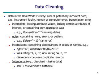
Data Cleaning
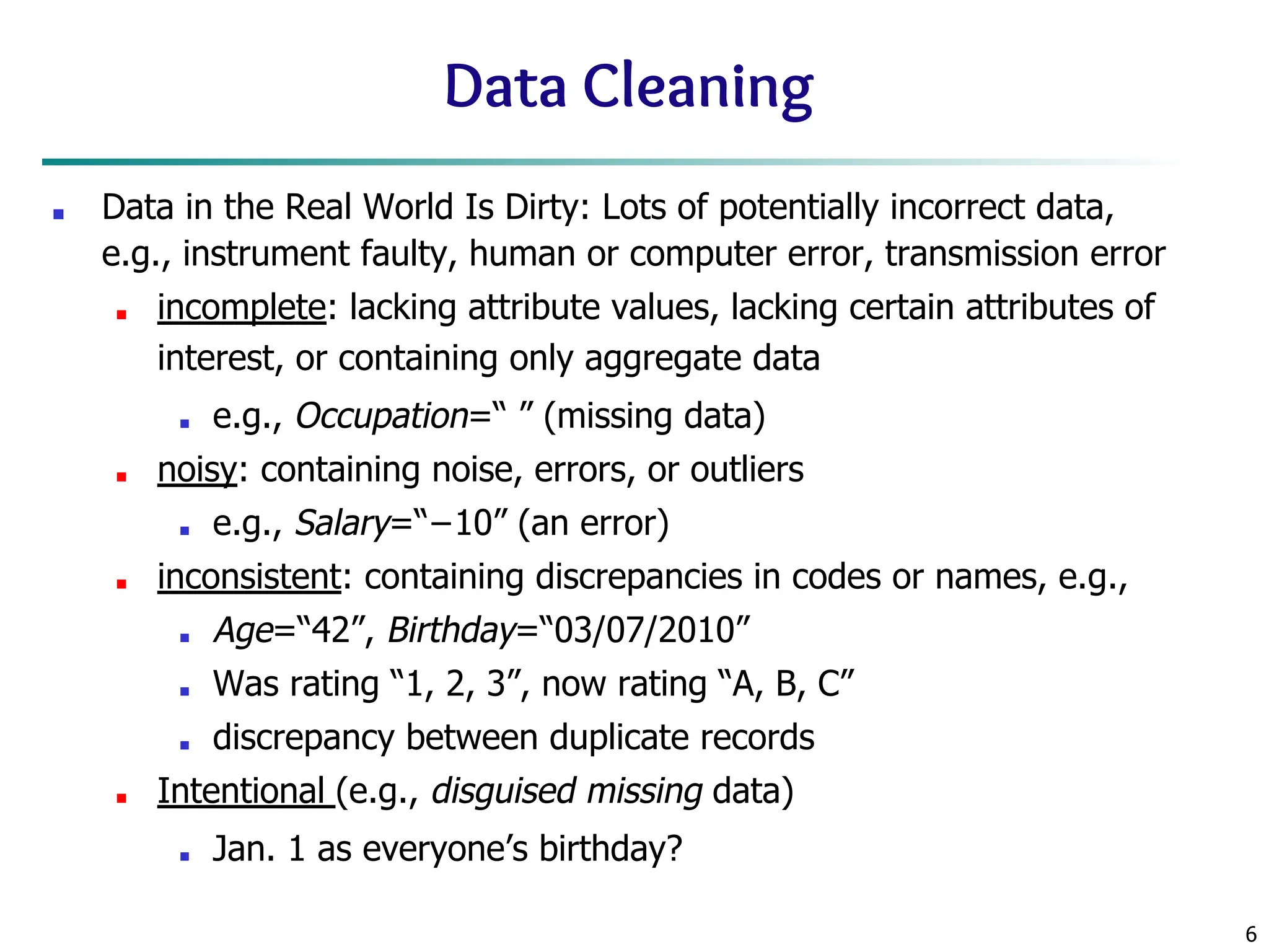
■ Datain the Real World Is Dirty: Lots of potentially incorrect data,
e.g., instrument faulty, human or computer error, transmission error
■ incomplete: lacking attribute values, lacking certain attributes of
interest, or containing only aggregate data
■ e.g., Occupation=“ ” (missing data)
■ noisy: containing noise, errors, or outliers
■ e.g., Salary=“−10” (an error)
■ inconsistent: containing discrepancies in codes or names, e.g.,
■ Age=“42”, Birthday=“03/07/2010”
■ Was rating “1, 2, 3”, now rating “A, B, C”
■ discrepancy between duplicate records
■ Intentional (e.g., disguised missing data)
■ Jan. 1 as everyone’s birthday?
7.
7
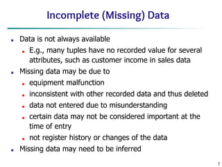
Incomplete (Missing) Data
■Data is not always available
■ E.g., many tuples have no recorded value for several
attributes, such as customer income in sales data
■ Missing data may be due to
■ equipment malfunction
■ inconsistent with other recorded data and thus deleted
■ data not entered due to misunderstanding
■ certain data may not be considered important at the
time of entry
■ not register history or changes of the data
■ Missing data may need to be inferred
8.
8
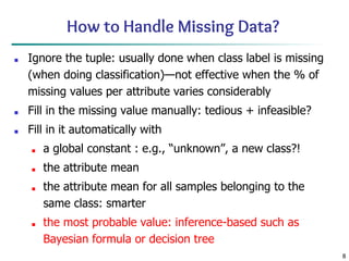
How to HandleMissing Data?
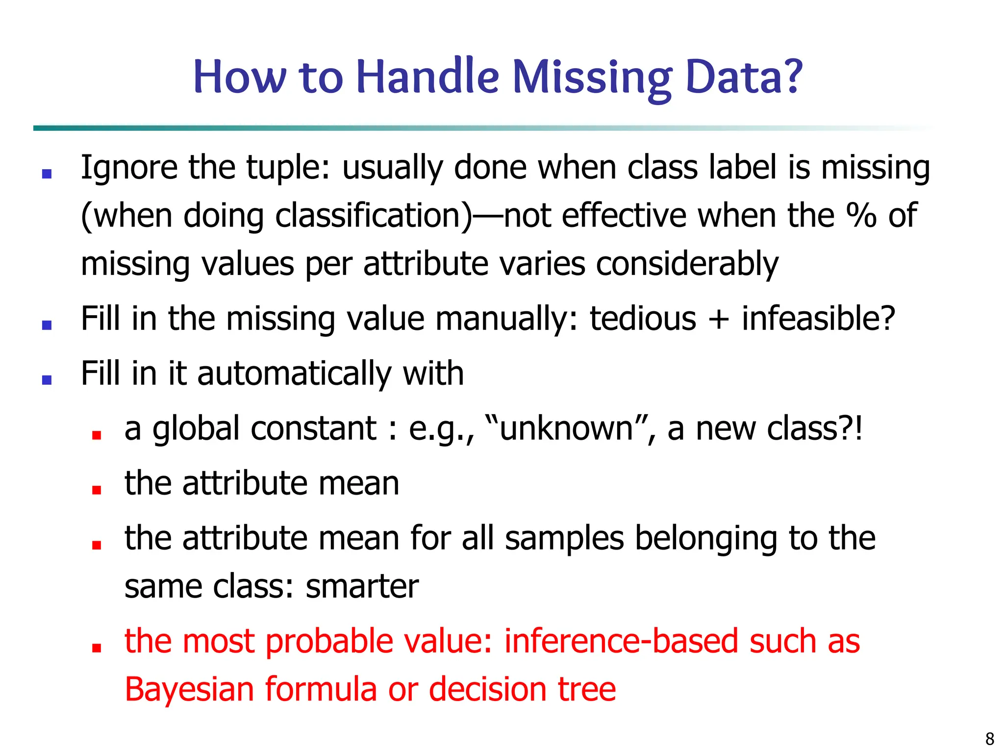
■ Ignore the tuple: usually done when class label is missing
(when doing classification)—not effective when the % of
missing values per attribute varies considerably
■ Fill in the missing value manually: tedious + infeasible?
■ Fill in it automatically with
■ a global constant : e.g., “unknown”, a new class?!
■ the attribute mean
■ the attribute mean for all samples belonging to the
same class: smarter
■ the most probable value: inference-based such as
Bayesian formula or decision tree
9.
9
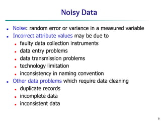
Noisy Data
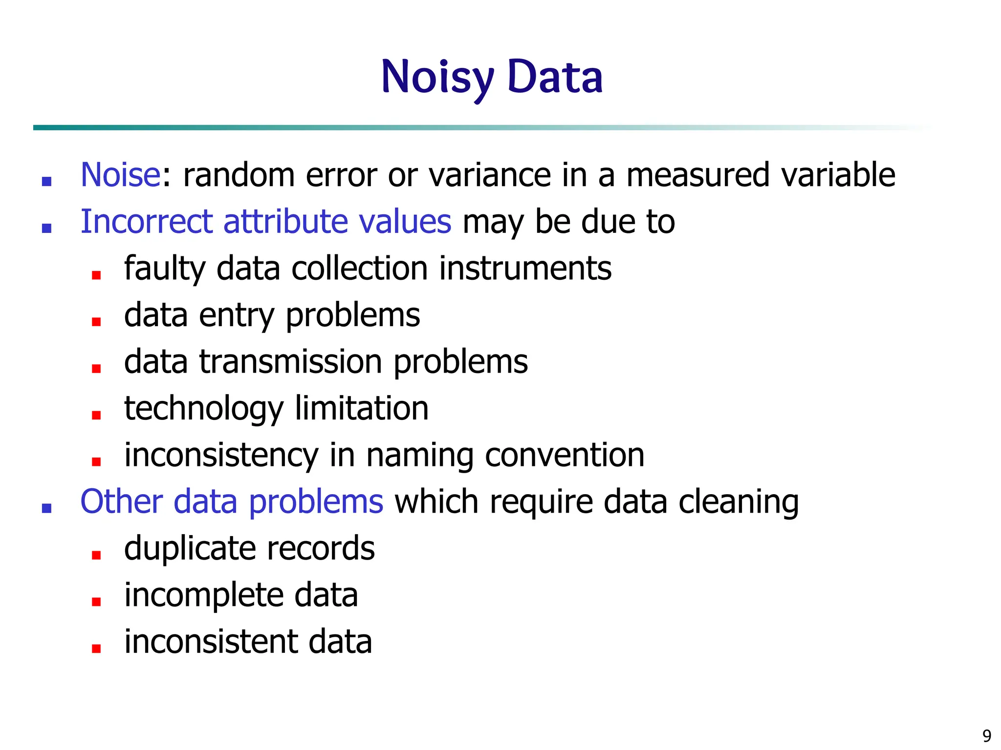
■ Noise:random error or variance in a measured variable
■ Incorrect attribute values may be due to
■ faulty data collection instruments
■ data entry problems
■ data transmission problems
■ technology limitation
■ inconsistency in naming convention
■ Other data problems which require data cleaning
■ duplicate records
■ incomplete data
■ inconsistent data
10.
10
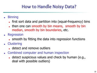
How to HandleNoisy Data?
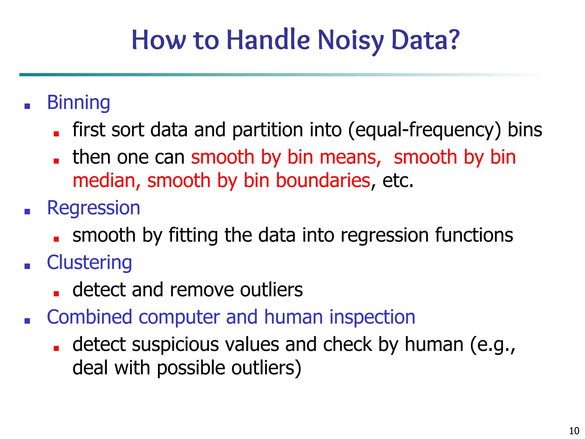
■ Binning
■ first sort data and partition into (equal-frequency) bins
■ then one can smooth by bin means, smooth by bin
median, smooth by bin boundaries, etc.
■ Regression
■ smooth by fitting the data into regression functions
■ Clustering
■ detect and remove outliers
■ Combined computer and human inspection
■ detect suspicious values and check by human (e.g.,
deal with possible outliers)
11.
11
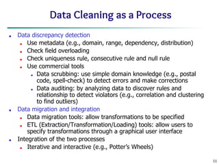
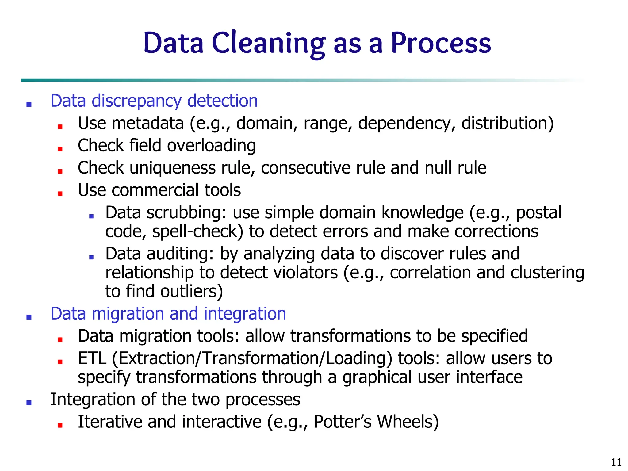
Data Cleaning asa Process
■ Data discrepancy detection
■ Use metadata (e.g., domain, range, dependency, distribution)
■ Check field overloading
■ Check uniqueness rule, consecutive rule and null rule
■ Use commercial tools
■ Data scrubbing: use simple domain knowledge (e.g., postal
code, spell-check) to detect errors and make corrections
■ Data auditing: by analyzing data to discover rules and
relationship to detect violators (e.g., correlation and clustering
to find outliers)
■ Data migration and integration
■ Data migration tools: allow transformations to be specified
■ ETL (Extraction/Transformation/Loading) tools: allow users to
specify transformations through a graphical user interface
■ Integration of the two processes
■ Iterative and interactive (e.g., Potter’s Wheels)
12.
12
12
Chapter 3: DataPreprocessing
■ Data Preprocessing: An Overview
■ Data Quality
■ Major Tasks in Data Preprocessing
■ Data Cleaning
■ Data Integration
■ Data Reduction
■ Data Transformation and Data Discretization
■ Summary
13.
13
13
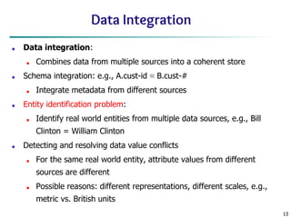
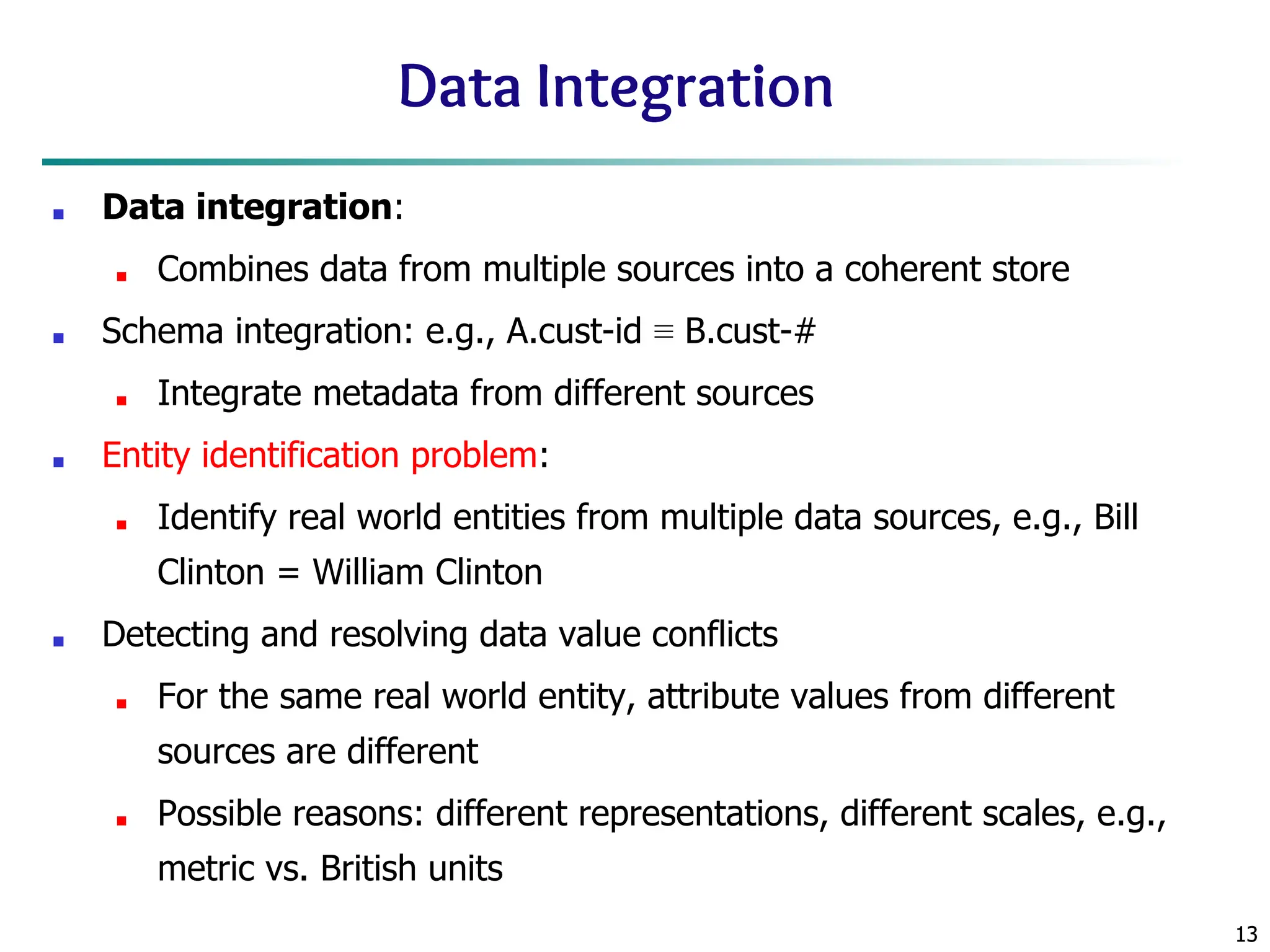
Data Integration
■ Dataintegration:
■ Combines data from multiple sources into a coherent store
■ Schema integration: e.g., A.cust-id ≡ B.cust-#
■ Integrate metadata from different sources
■ Entity identification problem:
■ Identify real world entities from multiple data sources, e.g., Bill
Clinton = William Clinton
■ Detecting and resolving data value conflicts
■ For the same real world entity, attribute values from different
sources are different
■ Possible reasons: different representations, different scales, e.g.,
metric vs. British units
14.
14
14
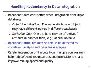
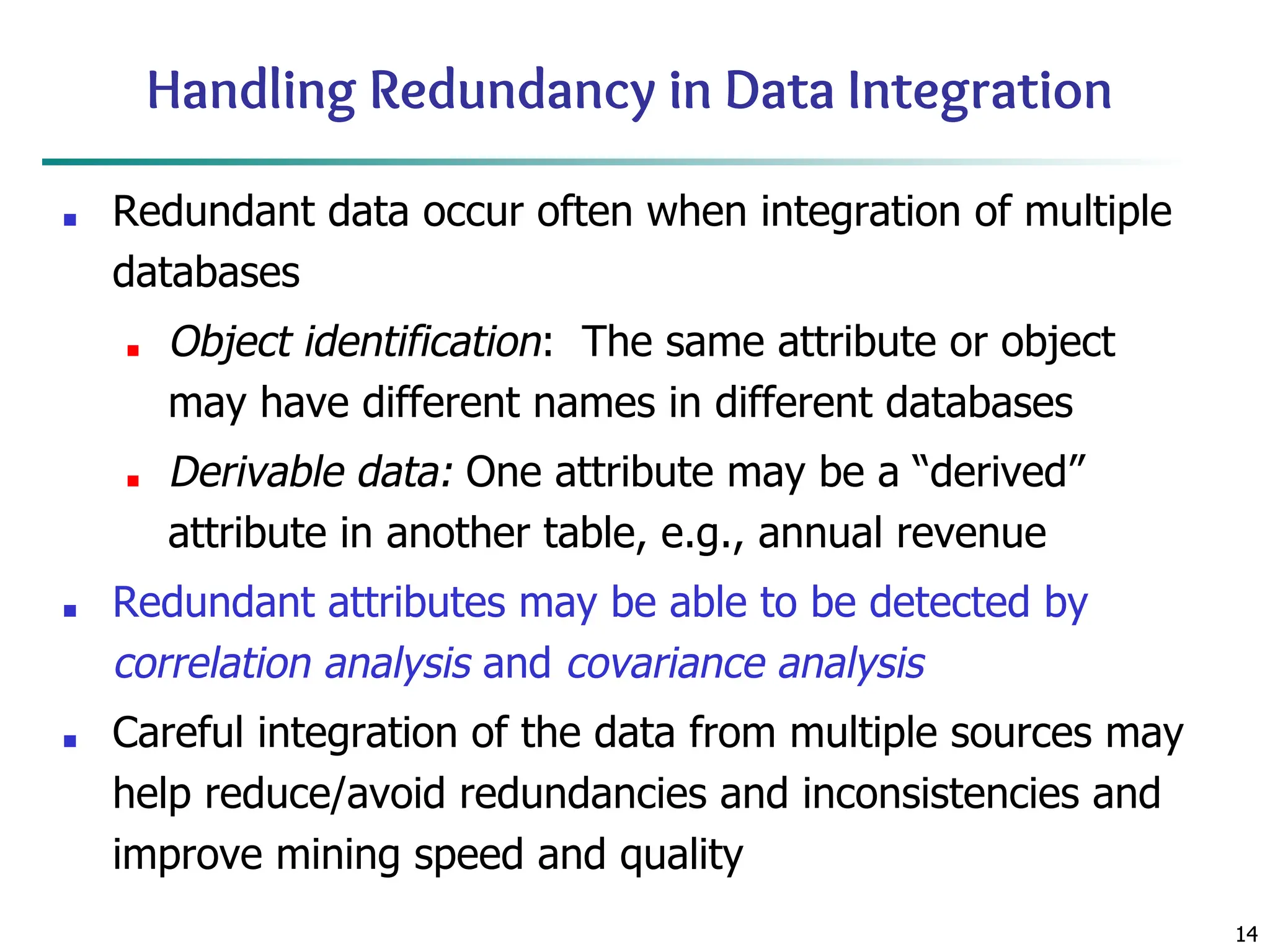
Handling Redundancy inData Integration
■ Redundant data occur often when integration of multiple
databases
■ Object identification: The same attribute or object
may have different names in different databases
■ Derivable data: One attribute may be a “derived”
attribute in another table, e.g., annual revenue
■ Redundant attributes may be able to be detected by
correlation analysis and covariance analysis
■ Careful integration of the data from multiple sources may
help reduce/avoid redundancies and inconsistencies and
improve mining speed and quality
15.
15
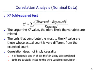
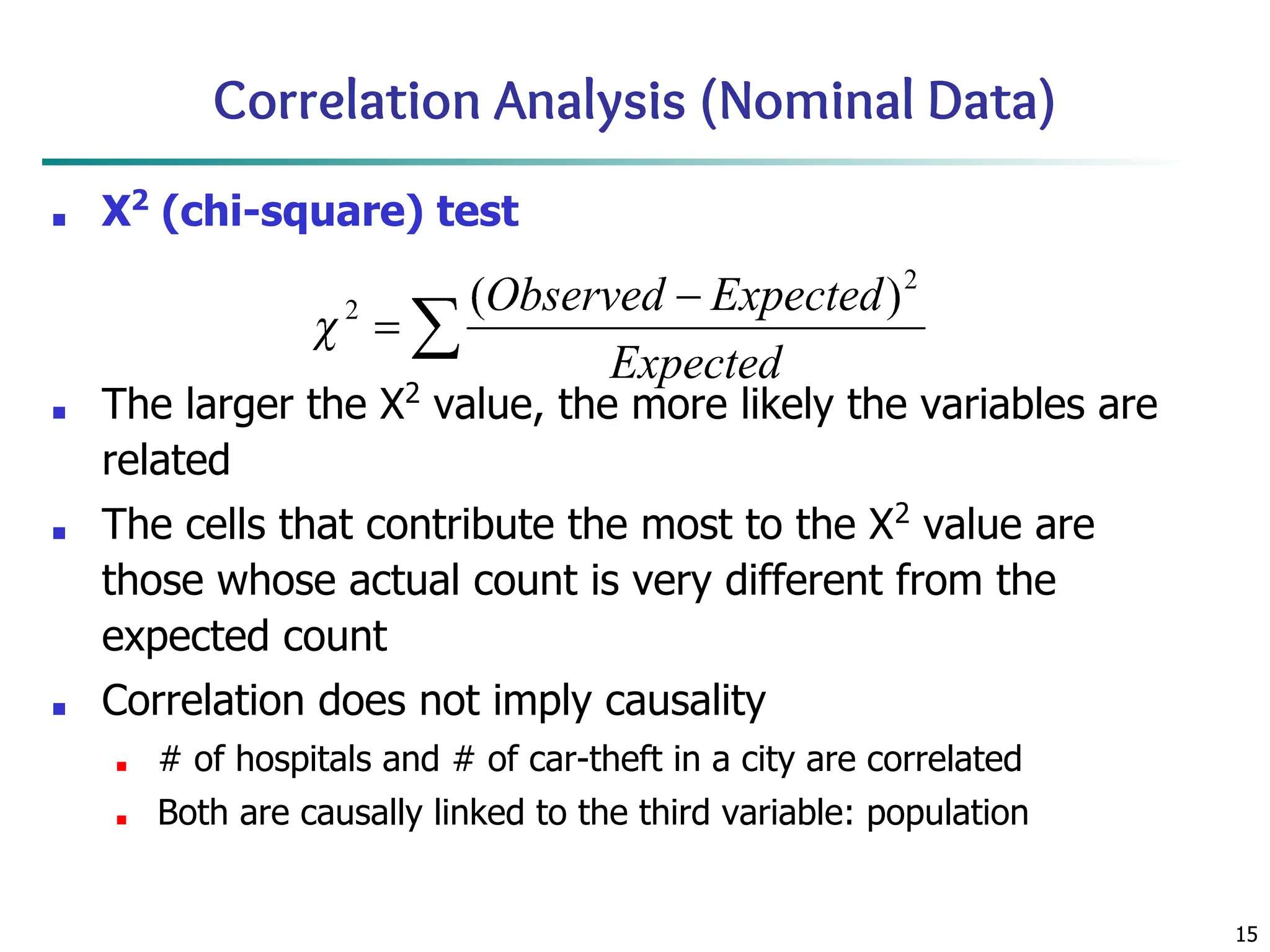
Correlation Analysis (NominalData)
■ Χ2
(chi-square) test
■ The larger the Χ2
value, the more likely the variables are
related
■ The cells that contribute the most to the Χ2
value are
those whose actual count is very different from the
expected count
■ Correlation does not imply causality
■ # of hospitals and # of car-theft in a city are correlated
■ Both are causally linked to the third variable: population
16.
16
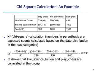
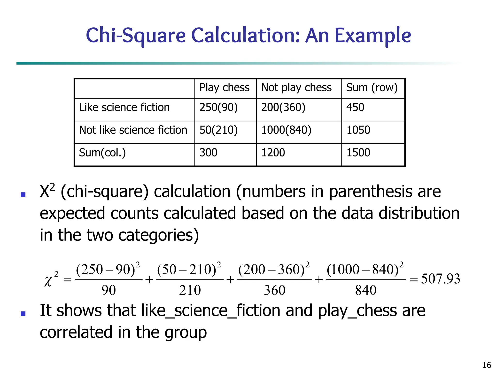
Chi-Square Calculation: AnExample
■ Χ2
(chi-square) calculation (numbers in parenthesis are
expected counts calculated based on the data distribution
in the two categories)
■ It shows that like_science_fiction and play_chess are
correlated in the group
Play chess Not play chess Sum (row)
Like science fiction 250(90) 200(360) 450
Not like science fiction 50(210) 1000(840) 1050
Sum(col.) 300 1200 1500
17.
17
Correlation Analysis (NumericData)
■ Correlation coefficient (also called Pearson’s product
moment coefficient)
where n is the number of tuples, and are the respective
means of A and B, σA
and σB
are the respective standard deviation
of A and B, and Σ(ai
bi
) is the sum of the AB cross-product.
■ If rA,B
> 0, A and B are positively correlated (A’s values
increase as B’s). The higher, the stronger correlation.
■ rA,B
= 0: independent; rAB
< 0: negatively correlated
19
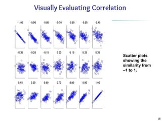
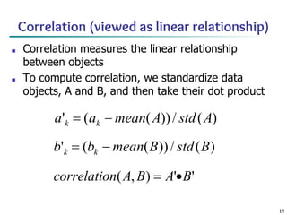
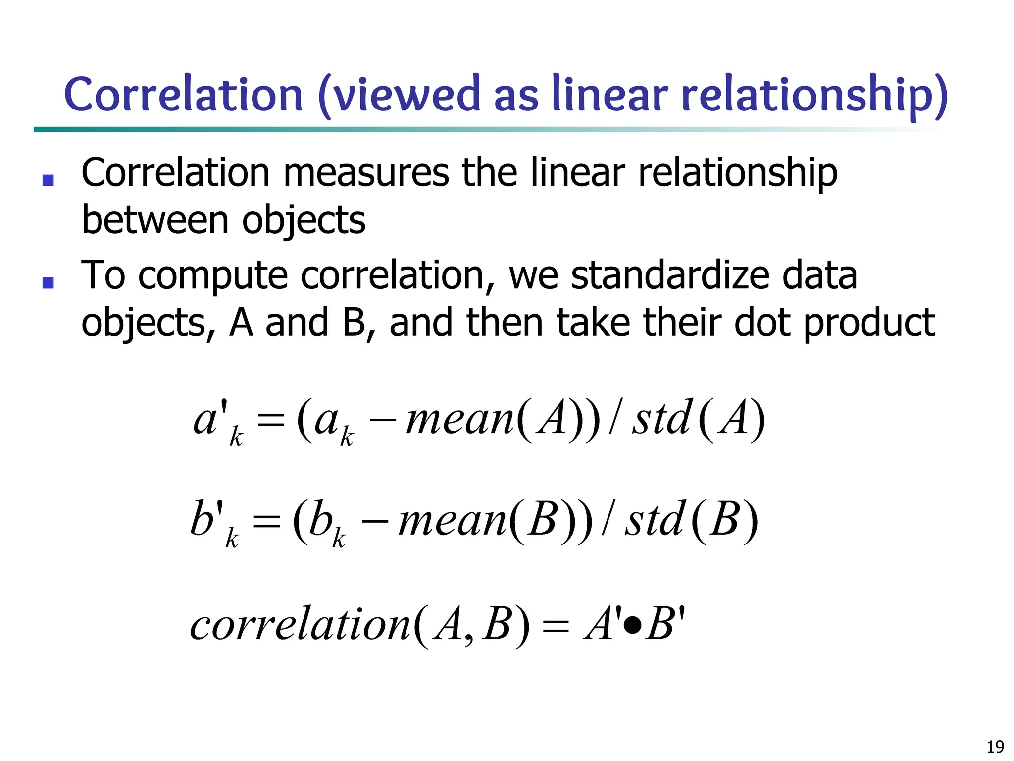
Correlation (viewed aslinear relationship)
■ Correlation measures the linear relationship
between objects
■ To compute correlation, we standardize data
objects, A and B, and then take their dot product
20.
20
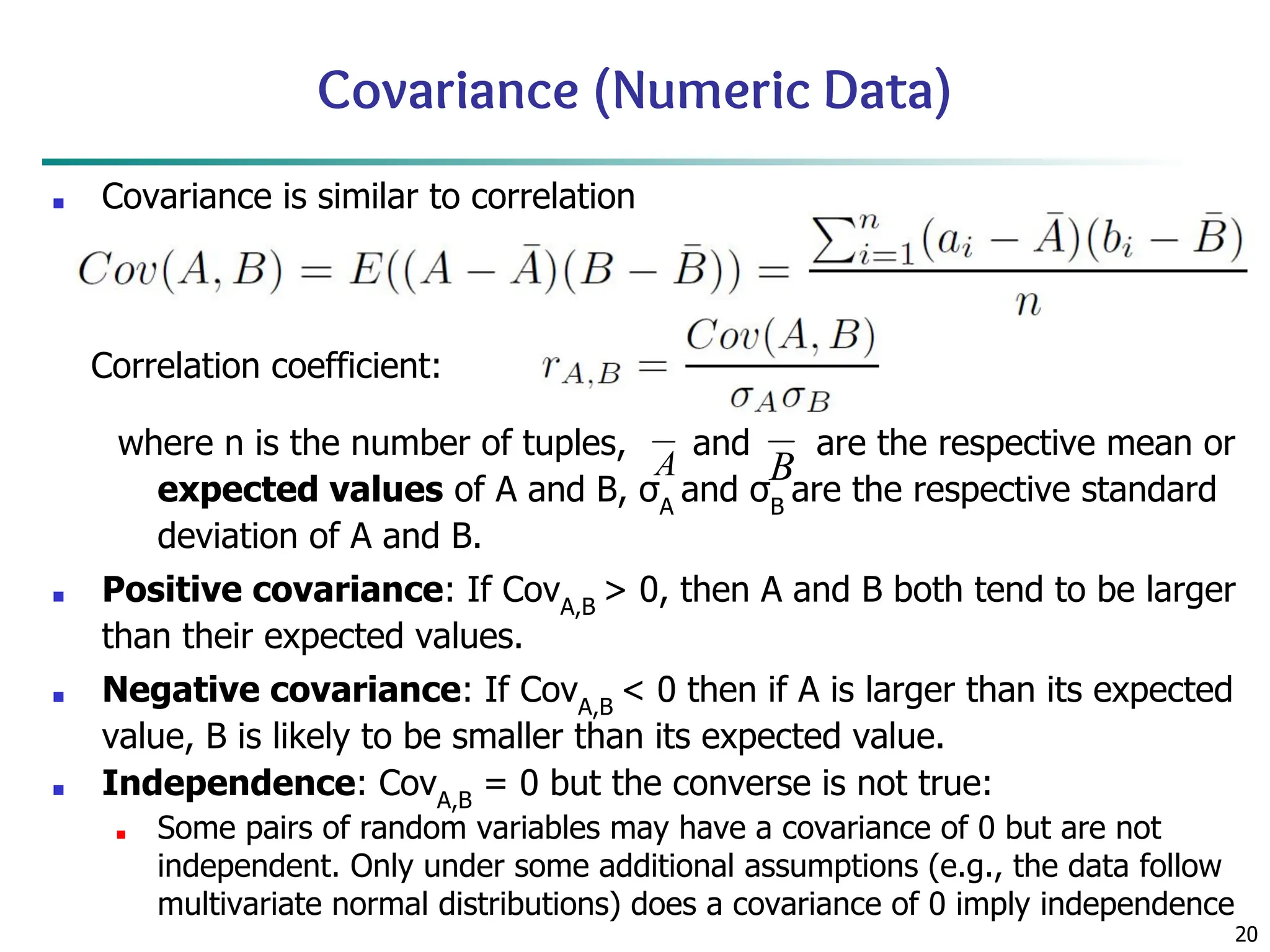
Covariance (Numeric Data)
■Covariance is similar to correlation
where n is the number of tuples, and are the respective mean or
expected values of A and B, σA
and σB
are the respective standard
deviation of A and B.
■ Positive covariance: If CovA,B
> 0, then A and B both tend to be larger
than their expected values.
■ Negative covariance: If CovA,B
< 0 then if A is larger than its expected
value, B is likely to be smaller than its expected value.
■ Independence: CovA,B
= 0 but the converse is not true:
■ Some pairs of random variables may have a covariance of 0 but are not
independent. Only under some additional assumptions (e.g., the data follow
multivariate normal distributions) does a covariance of 0 imply independence
Correlation coefficient:
21.
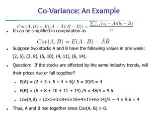
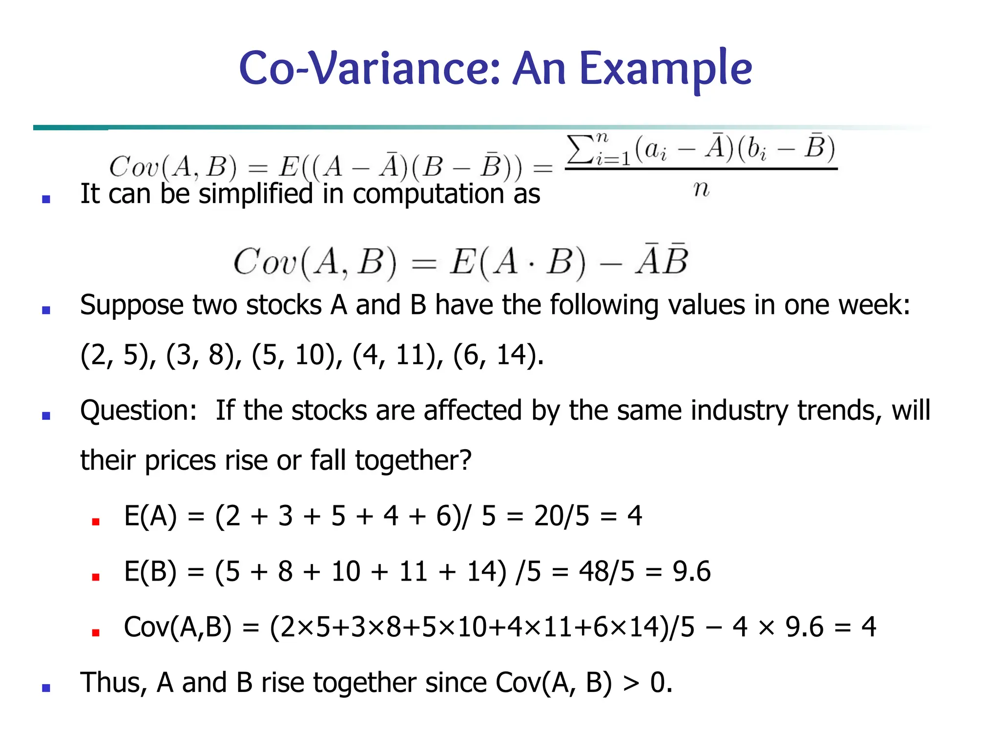
Co-Variance: An Example
■It can be simplified in computation as
■ Suppose two stocks A and B have the following values in one week:
(2, 5), (3, 8), (5, 10), (4, 11), (6, 14).
■ Question: If the stocks are affected by the same industry trends, will
their prices rise or fall together?
■ E(A) = (2 + 3 + 5 + 4 + 6)/ 5 = 20/5 = 4
■ E(B) = (5 + 8 + 10 + 11 + 14) /5 = 48/5 = 9.6
■ Cov(A,B) = (2×5+3×8+5×10+4×11+6×14)/5 − 4 × 9.6 = 4
■ Thus, A and B rise together since Cov(A, B) > 0.
22.
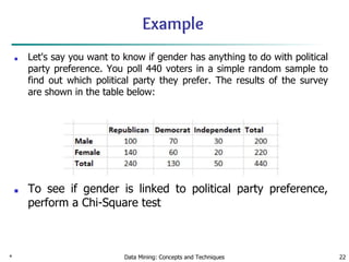
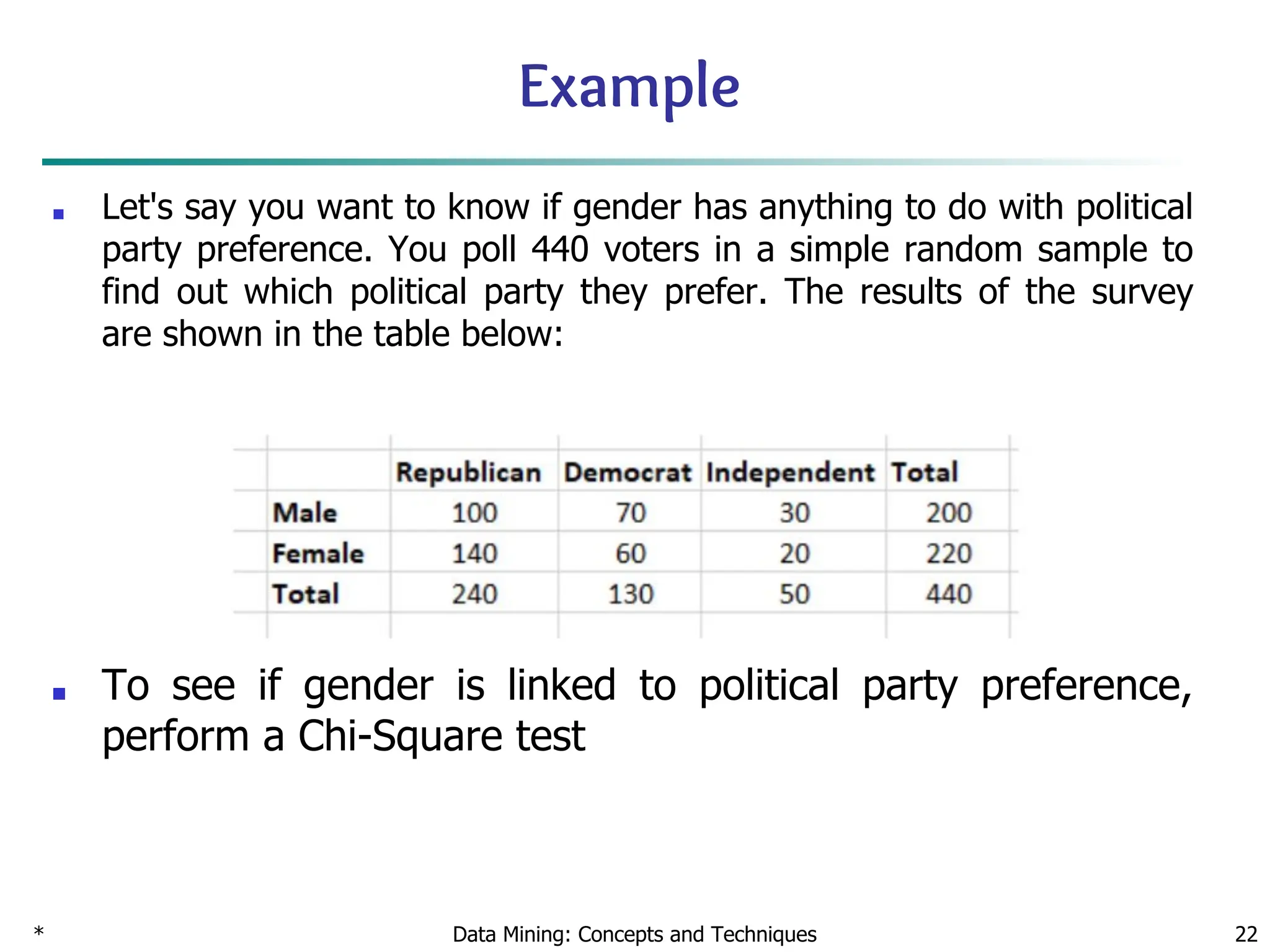
Example
■ Let's sayyou want to know if gender has anything to do with political
party preference. You poll 440 voters in a simple random sample to
find out which political party they prefer. The results of the survey
are shown in the table below:
■ To see if gender is linked to political party preference,
perform a Chi-Square test
* Data Mining: Concepts and Techniques 22
23.
23
23
Chapter 3: DataPreprocessing
■ Data Preprocessing: An Overview
■ Data Quality
■ Major Tasks in Data Preprocessing
■ Data Cleaning
■ Data Integration
■ Data Reduction
■ Data Transformation and Data Discretization
■ Summary
24.
24
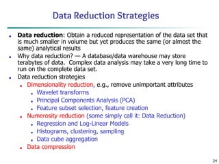
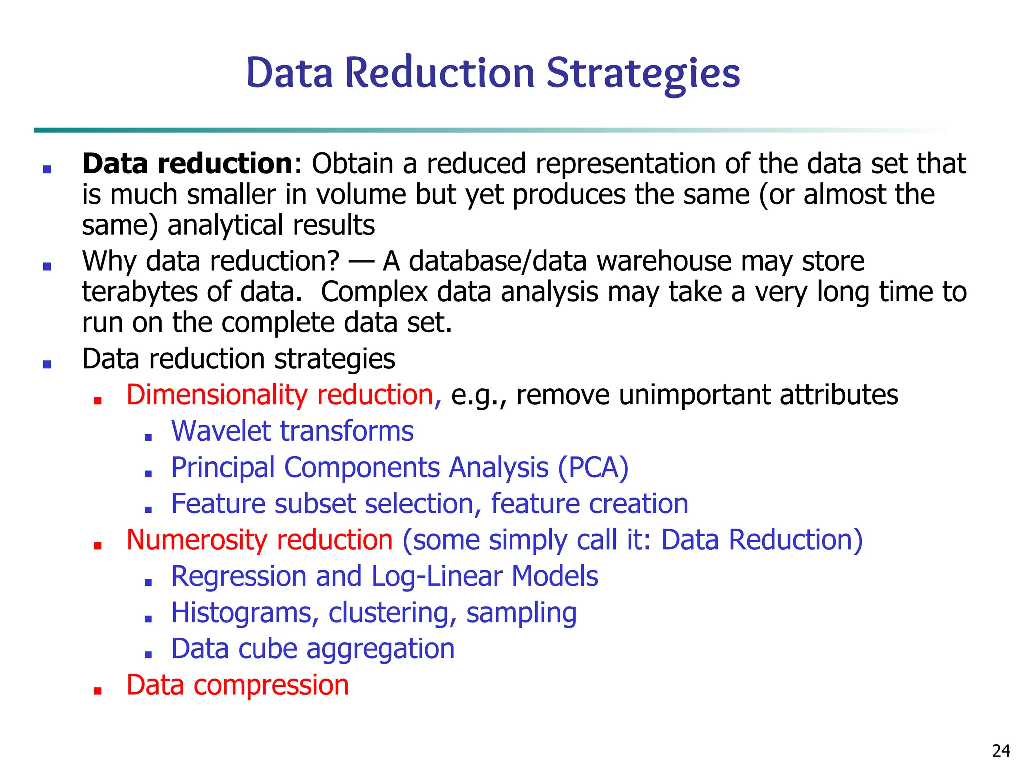
Data Reduction Strategies
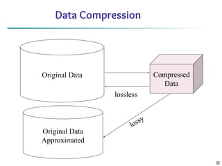
■Data reduction: Obtain a reduced representation of the data set that
is much smaller in volume but yet produces the same (or almost the
same) analytical results
■ Why data reduction? — A database/data warehouse may store
terabytes of data. Complex data analysis may take a very long time to
run on the complete data set.
■ Data reduction strategies
■ Dimensionality reduction, e.g., remove unimportant attributes
■ Wavelet transforms
■ Principal Components Analysis (PCA)
■ Feature subset selection, feature creation
■ Numerosity reduction (some simply call it: Data Reduction)
■ Regression and Log-Linear Models
■ Histograms, clustering, sampling
■ Data cube aggregation
■ Data compression
25.
25
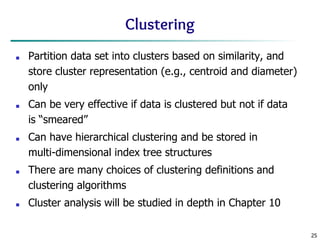
Clustering
■ Partition dataset into clusters based on similarity, and
store cluster representation (e.g., centroid and diameter)
only
■ Can be very effective if data is clustered but not if data
is “smeared”
■ Can have hierarchical clustering and be stored in
multi-dimensional index tree structures
■ There are many choices of clustering definitions and
clustering algorithms
■ Cluster analysis will be studied in depth in Chapter 10
26.
26
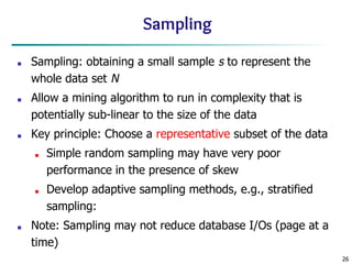
Sampling
■ Sampling: obtaininga small sample s to represent the
whole data set N
■ Allow a mining algorithm to run in complexity that is
potentially sub-linear to the size of the data
■ Key principle: Choose a representative subset of the data
■ Simple random sampling may have very poor
performance in the presence of skew
■ Develop adaptive sampling methods, e.g., stratified
sampling:
■ Note: Sampling may not reduce database I/Os (page at a
time)
27.
27
Types of Sampling
■Simple random sampling
■ There is an equal probability of selecting any particular
item
■ Sampling without replacement
■ Once an object is selected, it is removed from the
population
■ Sampling with replacement
■ A selected object is not removed from the population
■ Stratified sampling:
■ Partition the data set, and draw samples from each
partition (proportionally, i.e., approximately the same
percentage of the data)
■ Used in conjunction with skewed data
28.
28
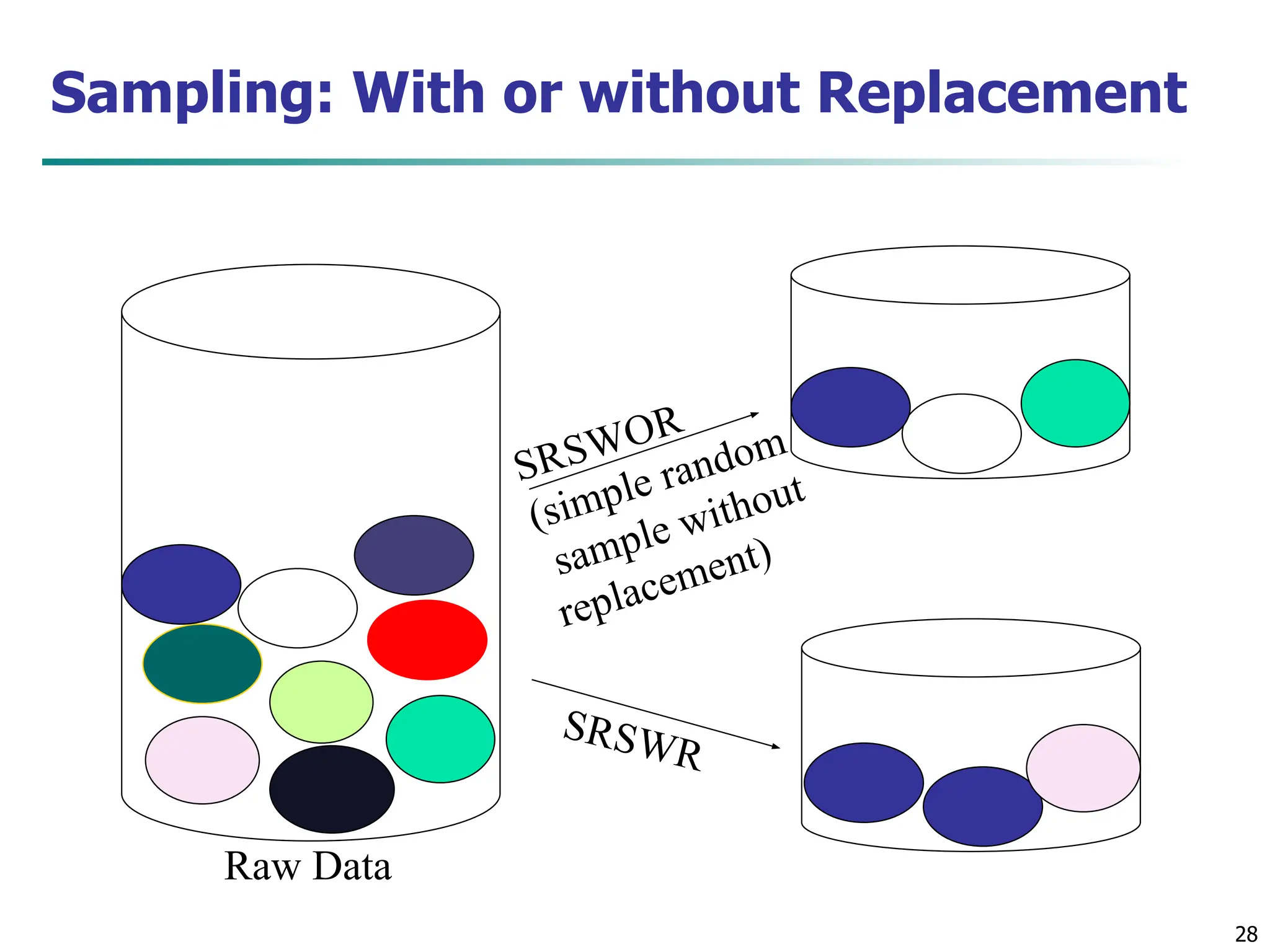
Sampling: With orwithout Replacement
SRSWOR
(simple random
sample without
replacement)
SRSWR
Raw Data
30
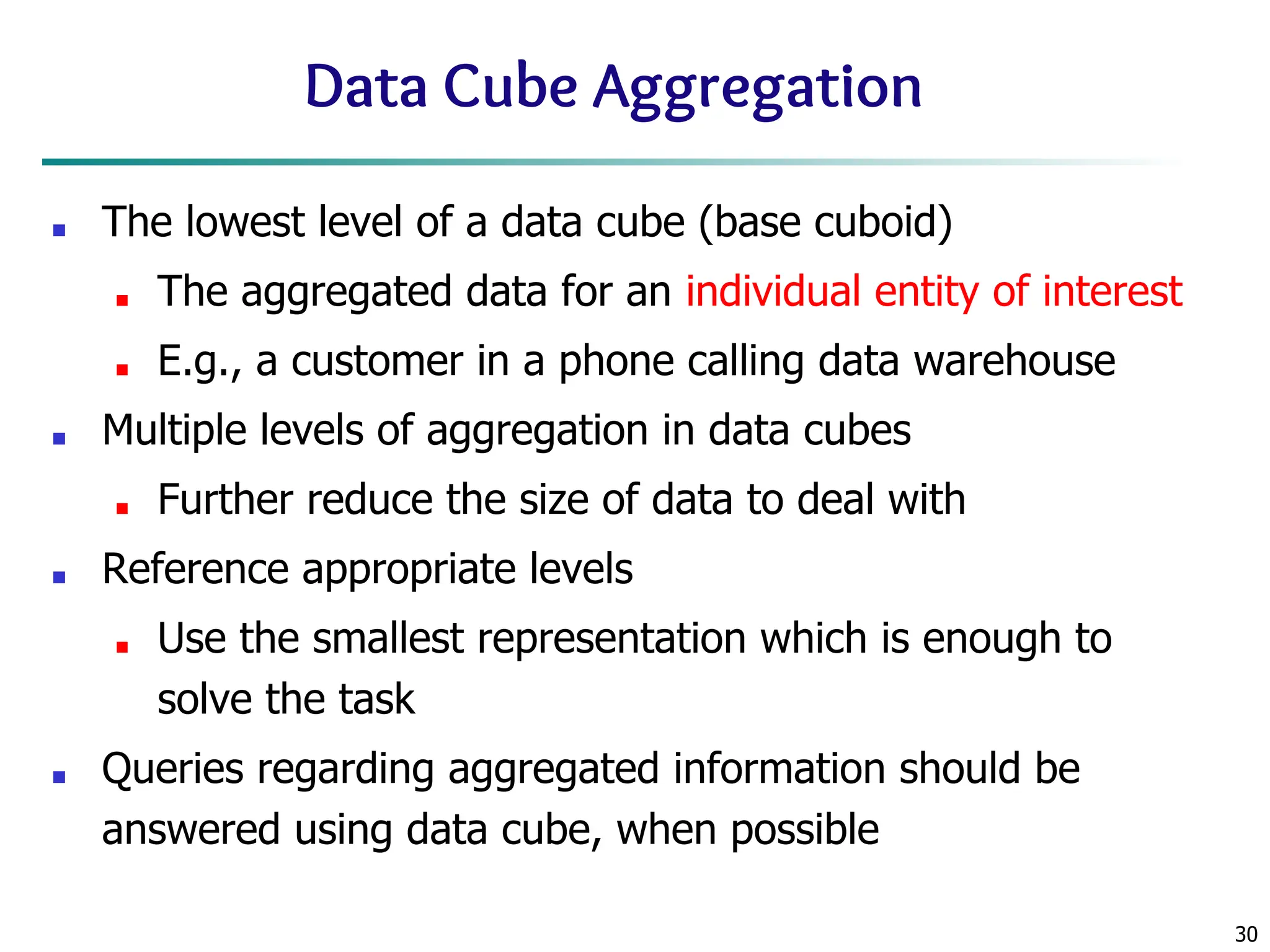
Data Cube Aggregation
■The lowest level of a data cube (base cuboid)
■ The aggregated data for an individual entity of interest
■ E.g., a customer in a phone calling data warehouse
■ Multiple levels of aggregation in data cubes
■ Further reduce the size of data to deal with
■ Reference appropriate levels
■ Use the smallest representation which is enough to
solve the task
■ Queries regarding aggregated information should be
answered using data cube, when possible
31.
31
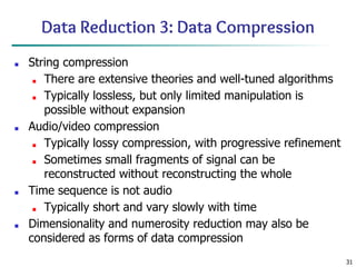
Data Reduction 3:Data Compression
■ String compression
■ There are extensive theories and well-tuned algorithms
■ Typically lossless, but only limited manipulation is
possible without expansion
■ Audio/video compression
■ Typically lossy compression, with progressive refinement
■ Sometimes small fragments of signal can be
reconstructed without reconstructing the whole
■ Time sequence is not audio
■ Typically short and vary slowly with time
■ Dimensionality and numerosity reduction may also be
considered as forms of data compression
33
Chapter 3: DataPreprocessing
■ Data Preprocessing: An Overview
■ Data Quality
■ Major Tasks in Data Preprocessing
■ Data Cleaning
■ Data Integration
■ Data Reduction
■ Data Transformation and Data Discretization
■ Summary
34.
34
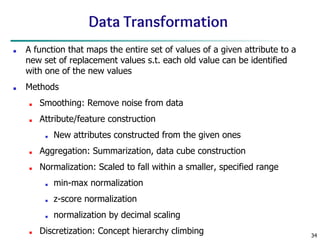
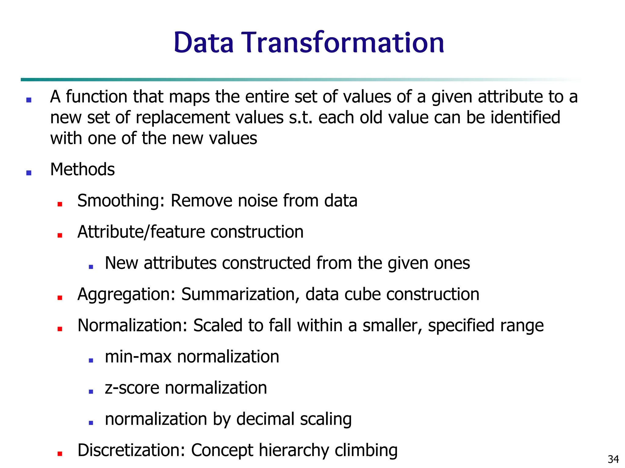
Data Transformation
■ Afunction that maps the entire set of values of a given attribute to a
new set of replacement values s.t. each old value can be identified
with one of the new values
■ Methods
■ Smoothing: Remove noise from data
■ Attribute/feature construction
■ New attributes constructed from the given ones
■ Aggregation: Summarization, data cube construction
■ Normalization: Scaled to fall within a smaller, specified range
■ min-max normalization
■ z-score normalization
■ normalization by decimal scaling
■ Discretization: Concept hierarchy climbing
35.
35
Normalization
■ Min-max normalization:to [new_minA
, new_maxA
]
■ Ex. Let income range $12,000 to $98,000 normalized to [0.0,
1.0]. Then $73,000 is mapped to
■ Z-score normalization (μ: mean, σ: standard deviation):
■ Ex. Let μ = 54,000, σ = 16,000. Then
■ Normalization by decimal scaling
Where j is the smallest integer such that Max(|ν’|) < 1
36.
36
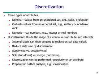
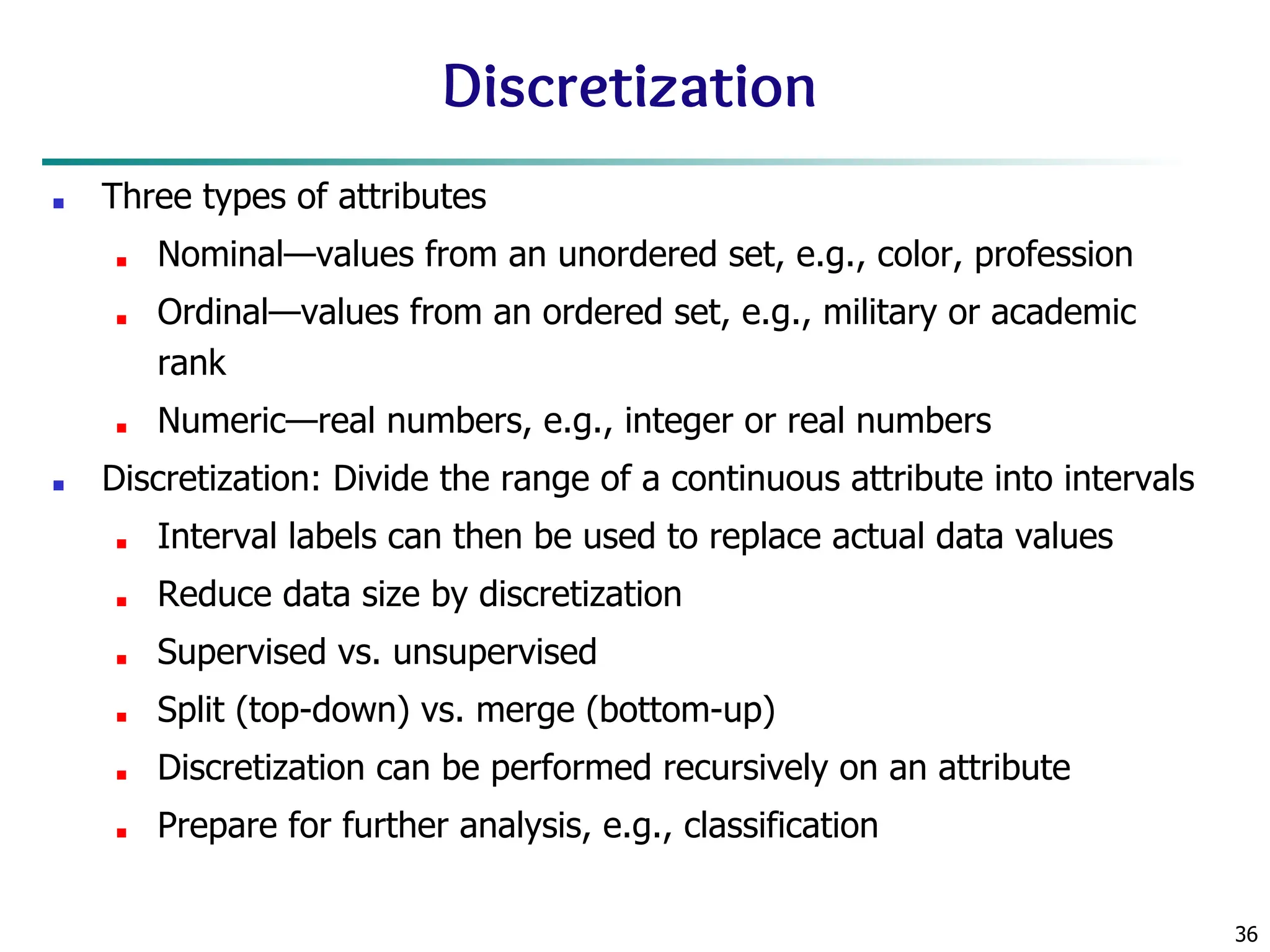
Discretization
■ Three typesof attributes
■ Nominal—values from an unordered set, e.g., color, profession
■ Ordinal—values from an ordered set, e.g., military or academic
rank
■ Numeric—real numbers, e.g., integer or real numbers
■ Discretization: Divide the range of a continuous attribute into intervals
■ Interval labels can then be used to replace actual data values
■ Reduce data size by discretization
■ Supervised vs. unsupervised
■ Split (top-down) vs. merge (bottom-up)
■ Discretization can be performed recursively on an attribute
■ Prepare for further analysis, e.g., classification
37.
37
Data Discretization Methods
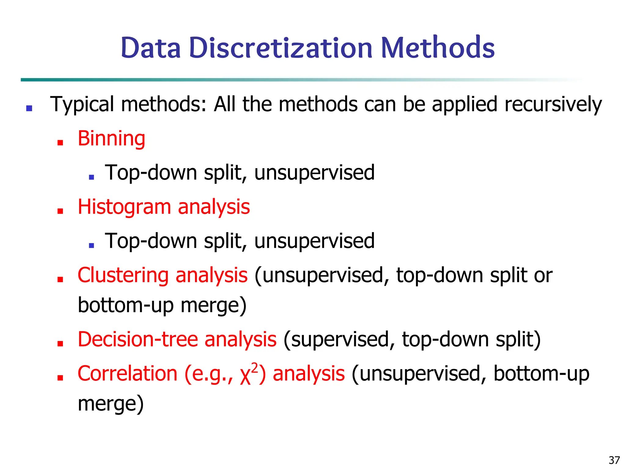
■Typical methods: All the methods can be applied recursively
■ Binning
■ Top-down split, unsupervised
■ Histogram analysis
■ Top-down split, unsupervised
■ Clustering analysis (unsupervised, top-down split or
bottom-up merge)
■ Decision-tree analysis (supervised, top-down split)
■ Correlation (e.g., χ2
) analysis (unsupervised, bottom-up
merge)
38.
38
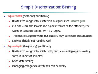
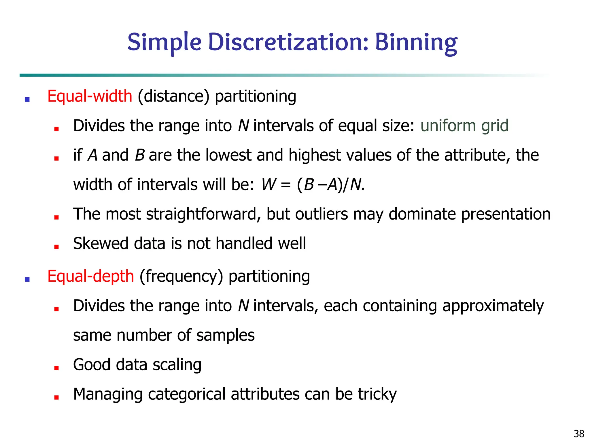
Simple Discretization: Binning
■Equal-width (distance) partitioning
■ Divides the range into N intervals of equal size: uniform grid
■ if A and B are the lowest and highest values of the attribute, the
width of intervals will be: W = (B –A)/N.
■ The most straightforward, but outliers may dominate presentation
■ Skewed data is not handled well
■ Equal-depth (frequency) partitioning
■ Divides the range into N intervals, each containing approximately
same number of samples
■ Good data scaling
■ Managing categorical attributes can be tricky
39.
39
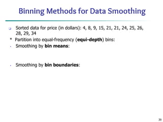
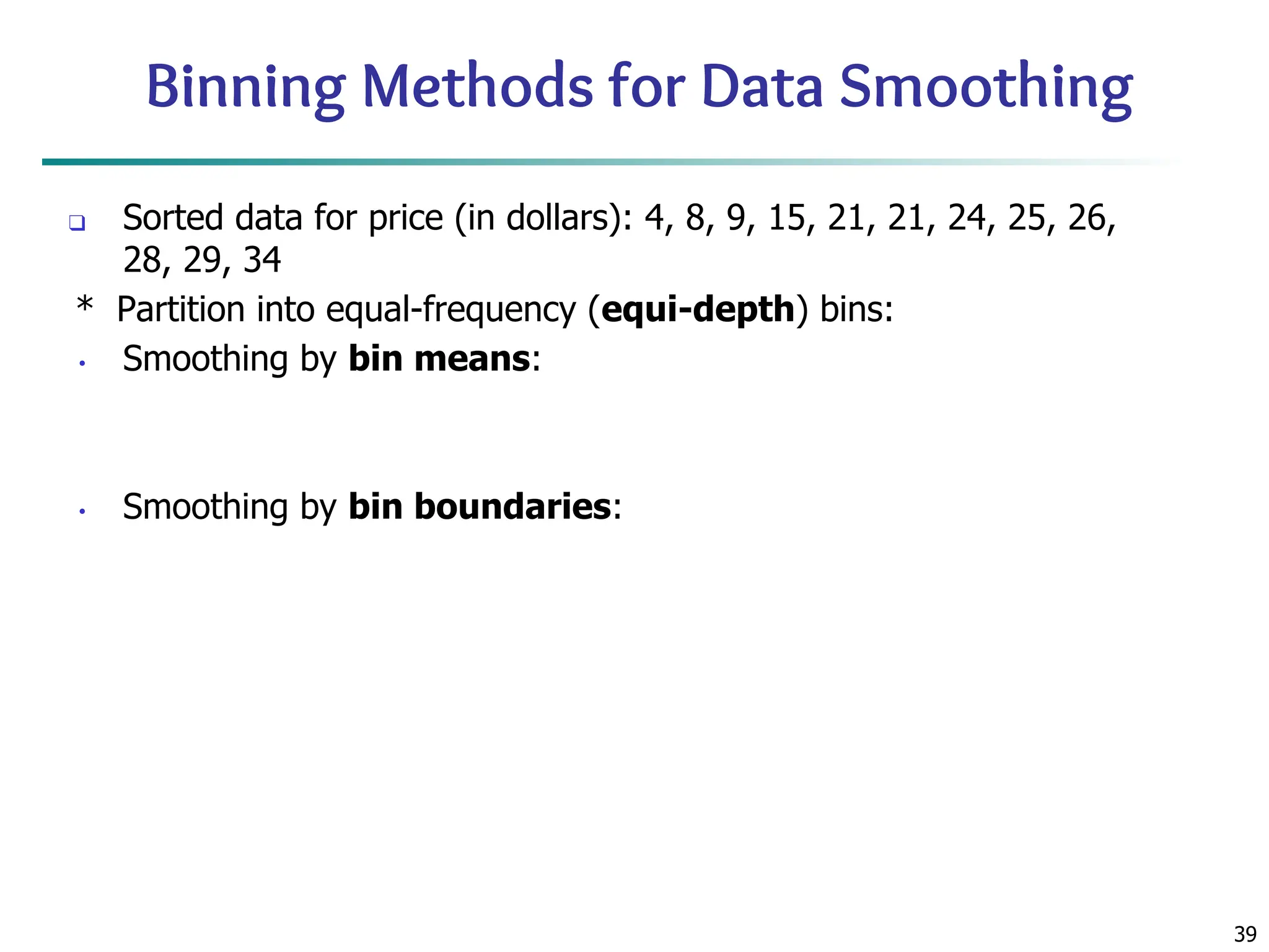
Binning Methods forData Smoothing
❑ Sorted data for price (in dollars): 4, 8, 9, 15, 21, 21, 24, 25, 26,
28, 29, 34
* Partition into equal-frequency (equi-depth) bins:
• Smoothing by bin means:
• Smoothing by bin boundaries:
40.
40
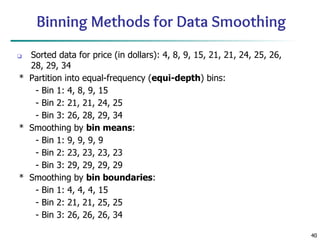
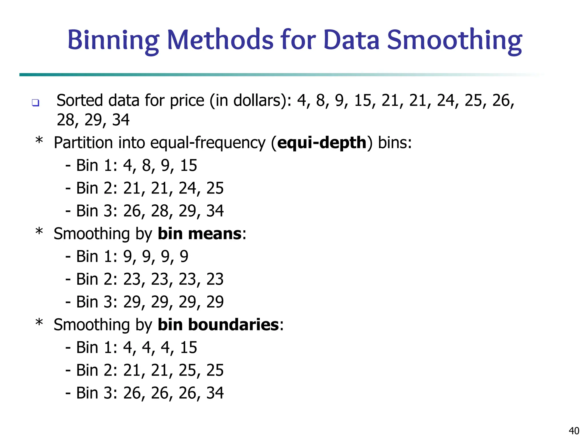
Binning Methods forData Smoothing
❑ Sorted data for price (in dollars): 4, 8, 9, 15, 21, 21, 24, 25, 26,
28, 29, 34
* Partition into equal-frequency (equi-depth) bins:
- Bin 1: 4, 8, 9, 15
- Bin 2: 21, 21, 24, 25
- Bin 3: 26, 28, 29, 34
* Smoothing by bin means:
- Bin 1: 9, 9, 9, 9
- Bin 2: 23, 23, 23, 23
- Bin 3: 29, 29, 29, 29
* Smoothing by bin boundaries:
- Bin 1: 4, 4, 4, 15
- Bin 2: 21, 21, 25, 25
- Bin 3: 26, 26, 26, 34
41.
41
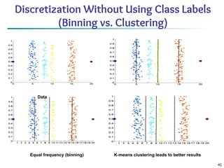
Discretization Without UsingClass Labels
(Binning vs. Clustering)
Data Equal interval width (binning)
Equal frequency (binning) K-means clustering leads to better results
42.
42
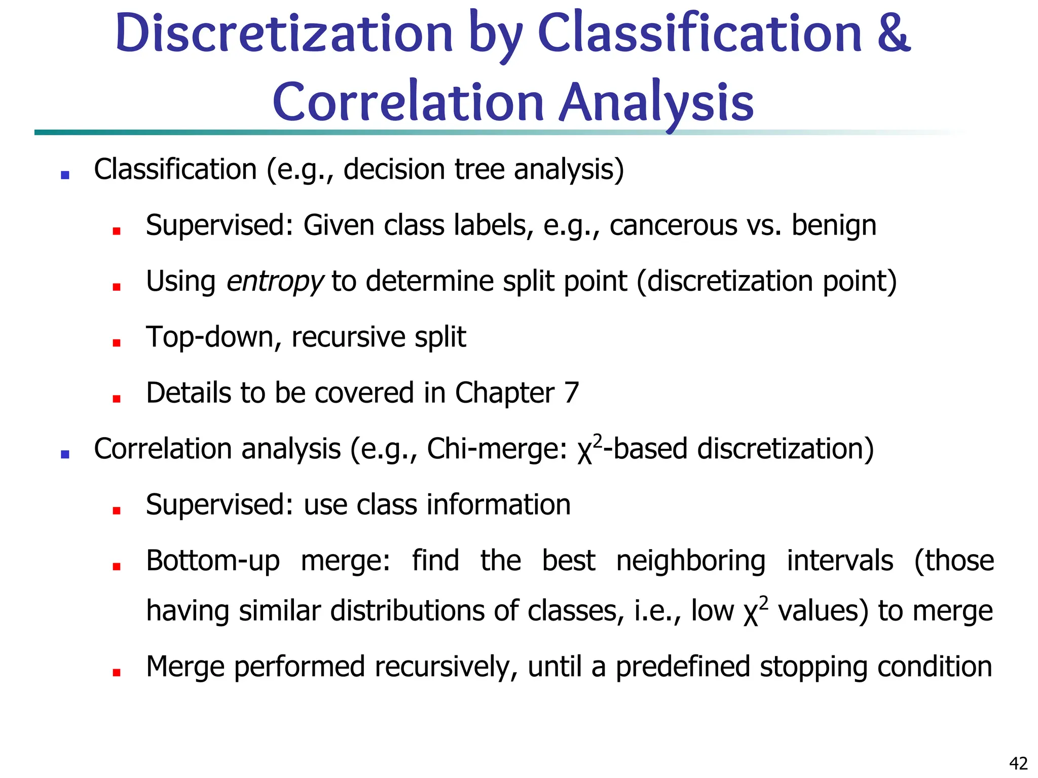
Discretization by Classification&
Correlation Analysis
■ Classification (e.g., decision tree analysis)
■ Supervised: Given class labels, e.g., cancerous vs. benign
■ Using entropy to determine split point (discretization point)
■ Top-down, recursive split
■ Details to be covered in Chapter 7
■ Correlation analysis (e.g., Chi-merge: χ2
-based discretization)
■ Supervised: use class information
■ Bottom-up merge: find the best neighboring intervals (those
having similar distributions of classes, i.e., low χ2
values) to merge
■ Merge performed recursively, until a predefined stopping condition
43.
43
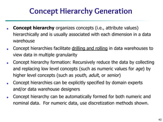
Concept Hierarchy Generation
■Concept hierarchy organizes concepts (i.e., attribute values)
hierarchically and is usually associated with each dimension in a data
warehouse
■ Concept hierarchies facilitate drilling and rolling in data warehouses to
view data in multiple granularity
■ Concept hierarchy formation: Recursively reduce the data by collecting
and replacing low level concepts (such as numeric values for age) by
higher level concepts (such as youth, adult, or senior)
■ Concept hierarchies can be explicitly specified by domain experts
and/or data warehouse designers
■ Concept hierarchy can be automatically formed for both numeric and
nominal data. For numeric data, use discretization methods shown.
44.
44
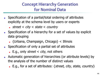
Concept Hierarchy Generation
forNominal Data
■ Specification of a partial/total ordering of attributes
explicitly at the schema level by users or experts
■ street < city < state < country
■ Specification of a hierarchy for a set of values by explicit
data grouping
■ {Urbana, Champaign, Chicago} < Illinois
■ Specification of only a partial set of attributes
■ E.g., only street < city, not others
■ Automatic generation of hierarchies (or attribute levels) by
the analysis of the number of distinct values
■ E.g., for a set of attributes: {street, city, state, country}
45.
45
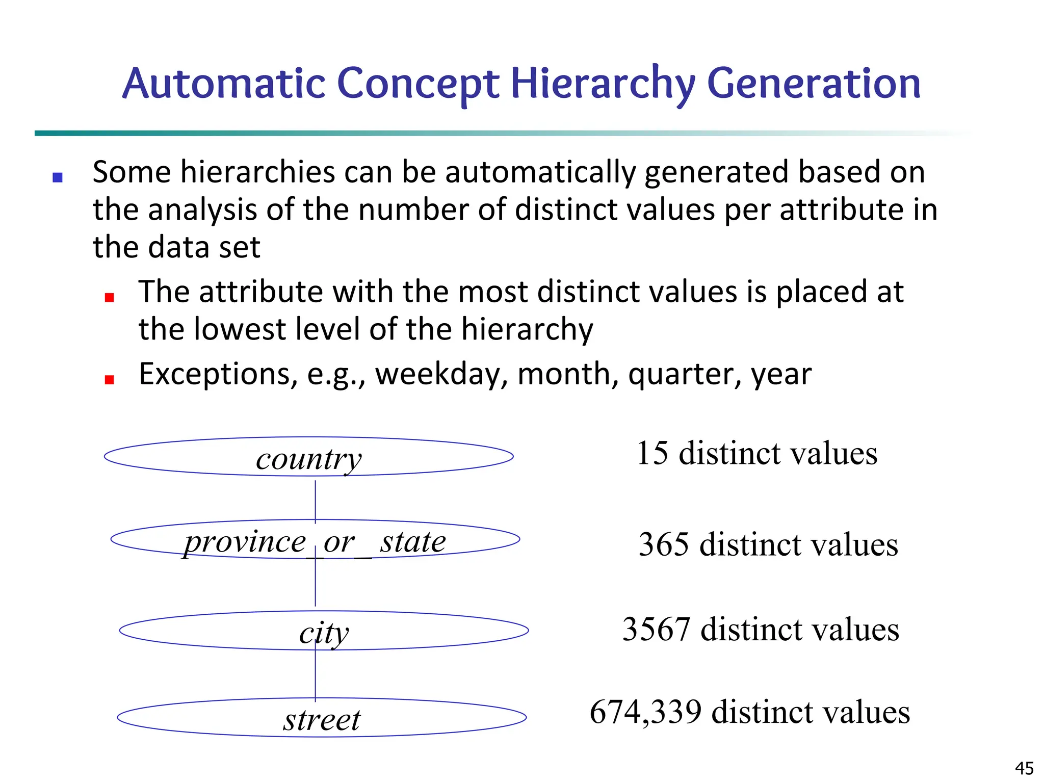
Automatic Concept HierarchyGeneration
■ Some hierarchies can be automatically generated based on
the analysis of the number of distinct values per attribute in
the data set
■ The attribute with the most distinct values is placed at
the lowest level of the hierarchy
■ Exceptions, e.g., weekday, month, quarter, year
country
province_or_ state
city
street
15 distinct values
365 distinct values
3567 distinct values
674,339 distinct values
46.
46
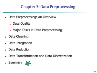
Chapter 3: DataPreprocessing
■ Data Preprocessing: An Overview
■ Data Quality
■ Major Tasks in Data Preprocessing
■ Data Cleaning
■ Data Integration
■ Data Reduction
■ Data Transformation and Data Discretization
■ Summary
47.
47
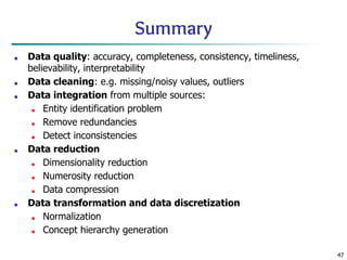
Summary
■ Data quality:accuracy, completeness, consistency, timeliness,
believability, interpretability
■ Data cleaning: e.g. missing/noisy values, outliers
■ Data integration from multiple sources:
■ Entity identification problem
■ Remove redundancies
■ Detect inconsistencies
■ Data reduction
■ Dimensionality reduction
■ Numerosity reduction
■ Data compression
■ Data transformation and data discretization
■ Normalization
■ Concept hierarchy generation
48.
48
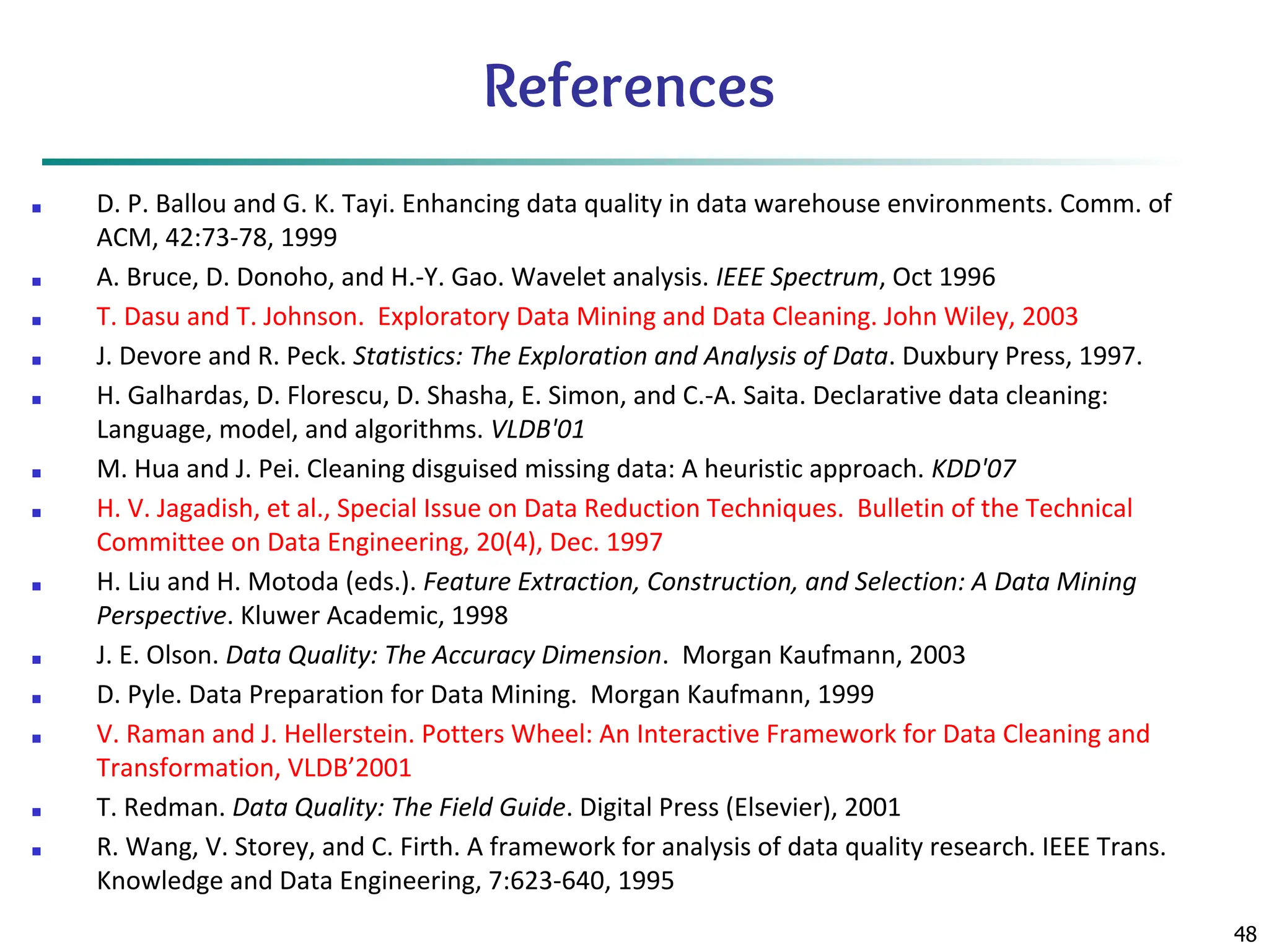
References
■ D. P.Ballou and G. K. Tayi. Enhancing data quality in data warehouse environments. Comm. of
ACM, 42:73-78, 1999
■ A. Bruce, D. Donoho, and H.-Y. Gao. Wavelet analysis. IEEE Spectrum, Oct 1996
■ T. Dasu and T. Johnson. Exploratory Data Mining and Data Cleaning. John Wiley, 2003
■ J. Devore and R. Peck. Statistics: The Exploration and Analysis of Data. Duxbury Press, 1997.
■ H. Galhardas, D. Florescu, D. Shasha, E. Simon, and C.-A. Saita. Declarative data cleaning:
Language, model, and algorithms. VLDB'01
■ M. Hua and J. Pei. Cleaning disguised missing data: A heuristic approach. KDD'07
■ H. V. Jagadish, et al., Special Issue on Data Reduction Techniques. Bulletin of the Technical
Committee on Data Engineering, 20(4), Dec. 1997
■ H. Liu and H. Motoda (eds.). Feature Extraction, Construction, and Selection: A Data Mining
Perspective. Kluwer Academic, 1998
■ J. E. Olson. Data Quality: The Accuracy Dimension. Morgan Kaufmann, 2003
■ D. Pyle. Data Preparation for Data Mining. Morgan Kaufmann, 1999
■ V. Raman and J. Hellerstein. Potters Wheel: An Interactive Framework for Data Cleaning and
Transformation, VLDB’2001
■ T. Redman. Data Quality: The Field Guide. Digital Press (Elsevier), 2001
■ R. Wang, V. Storey, and C. Firth. A framework for analysis of data quality research. IEEE Trans.
Knowledge and Data Engineering, 7:623-640, 1995


![35
Normalization
■ Min-max normalization: to [new_minA
, new_maxA
]
■ Ex. Let income range $12,000 to $98,000 normalized to [0.0,
1.0]. Then $73,000 is mapped to
■ Z-score normalization (μ: mean, σ: standard deviation):
■ Ex. Let μ = 54,000, σ = 16,000. Then
■ Normalization by decimal scaling
Where j is the smallest integer such that Max(|ν’|) < 1](https://image.slidesharecdn.com/6-250531064758-4739bbc0/85/Preprocessing-Step-in-Data-Cleaning-Data-Mining-35-320.jpg)


![35
Normalization
■ Min-max normalization: to [new_minA
, new_maxA
]
■ Ex. Let income range $12,000 to $98,000 normalized to [0.0,
1.0]. Then $73,000 is mapped to
■ Z-score normalization (μ: mean, σ: standard deviation):
■ Ex. Let μ = 54,000, σ = 16,000. Then
■ Normalization by decimal scaling
Where j is the smallest integer such that Max(|ν’|) < 1](https://image.slidesharecdn.com/6-250531064758-4739bbc0/75/Preprocessing-Step-in-Data-Cleaning-Data-Mining-35-2048.jpg)


![UiPath Automation Suite Installation (Hands-On) [2/3]](https://cdn.slidesharecdn.com/ss_thumbnails/automationsuitecommunitysession2-251015095633-a6d862f1-thumbnail.jpg?width=600ounds&width=560&fit=bounds)


