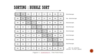
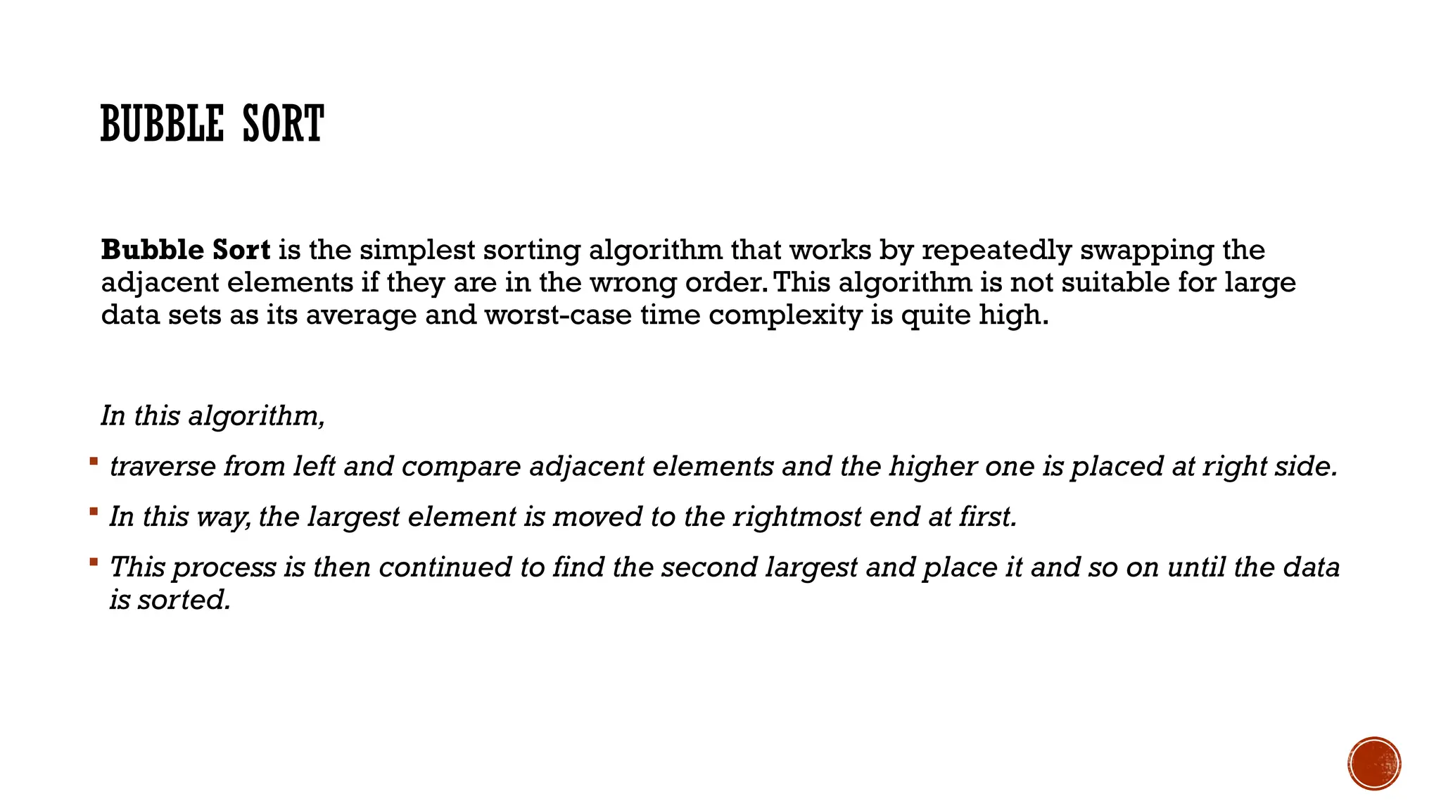
BUBBLE SORT
Bubble Sortis the simplest sorting algorithm that works by repeatedly swapping the
adjacent elements if they are in the wrong order.This algorithm is not suitable for large
data sets as its average and worst-case time complexity is quite high.
In this algorithm,
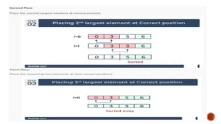
traverse from left and compare adjacent elements and the higher one is placed at right side.
In this way, the largest element is moved to the rightmost end at first.
This process is then continued to find the second largest and place it and so on until the data
is sorted.
SORTING ; BUBBLESORT
Algorithm: (Bubble Sort) BUBBLE(DATA,N)
Here DATA is a array with N elements.This
algorithm sorts the elements in DATA.
1. Repeat for PASS = 1 to N-1.
2. Repeat for i=0 to N-PASS.
3. If DATA[i] > DATA[i+1] then,
Interchange DATA[i] and DATA[i+1]
[End of IF structure]
[End of inner loop]
[End of Step 1 outer loop]
4. Exit.
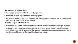
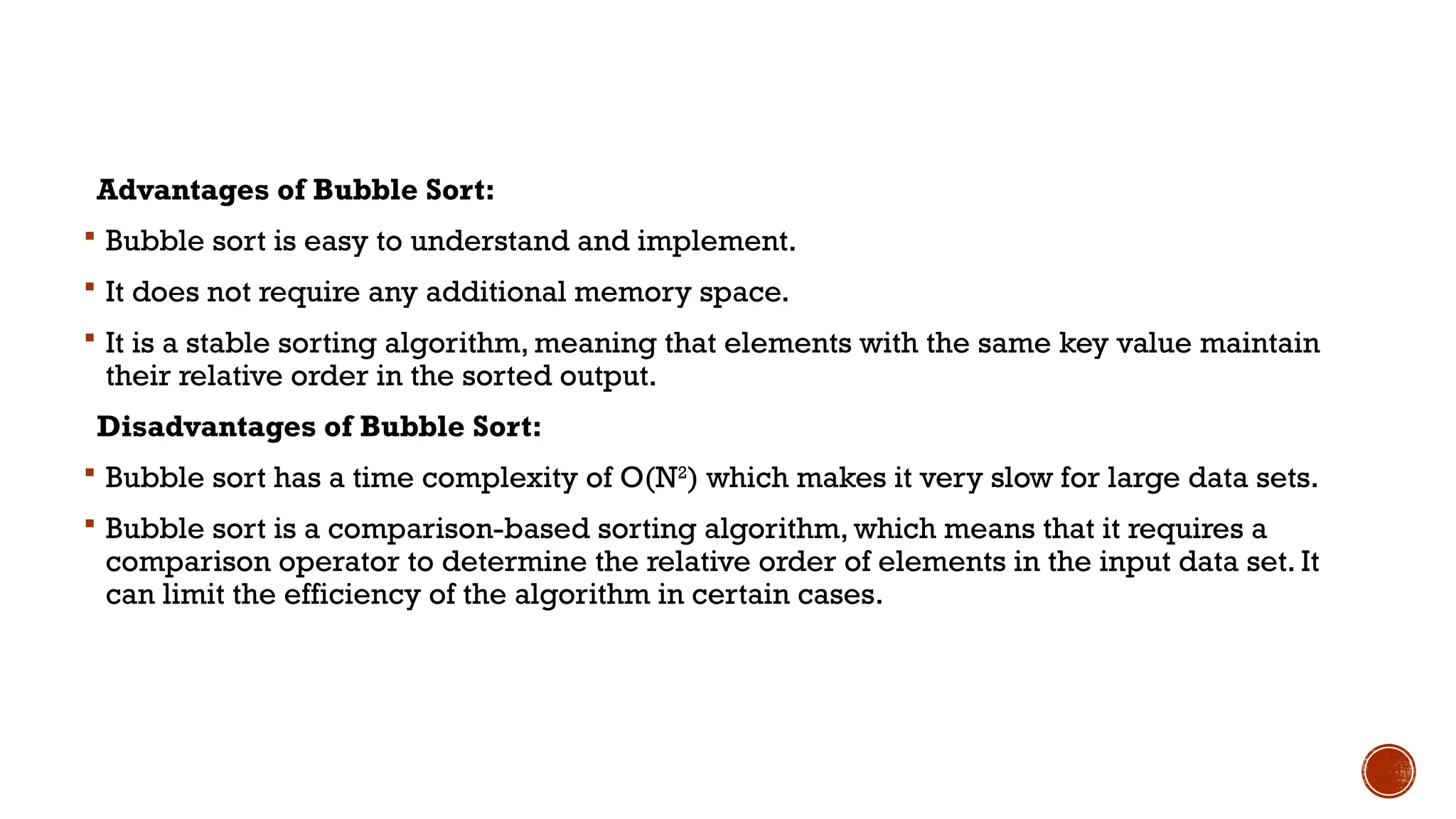
Advantages of BubbleSort:
Bubble sort is easy to understand and implement.
It does not require any additional memory space.
It is a stable sorting algorithm, meaning that elements with the same key value maintain
their relative order in the sorted output.
Disadvantages of Bubble Sort:
Bubble sort has a time complexity of O(N2
) which makes it very slow for large data sets.
Bubble sort is a comparison-based sorting algorithm, which means that it requires a
comparison operator to determine the relative order of elements in the input data set. It
can limit the efficiency of the algorithm in certain cases.
10.
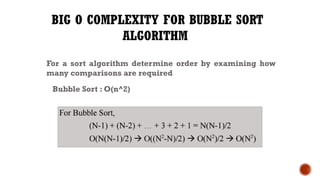
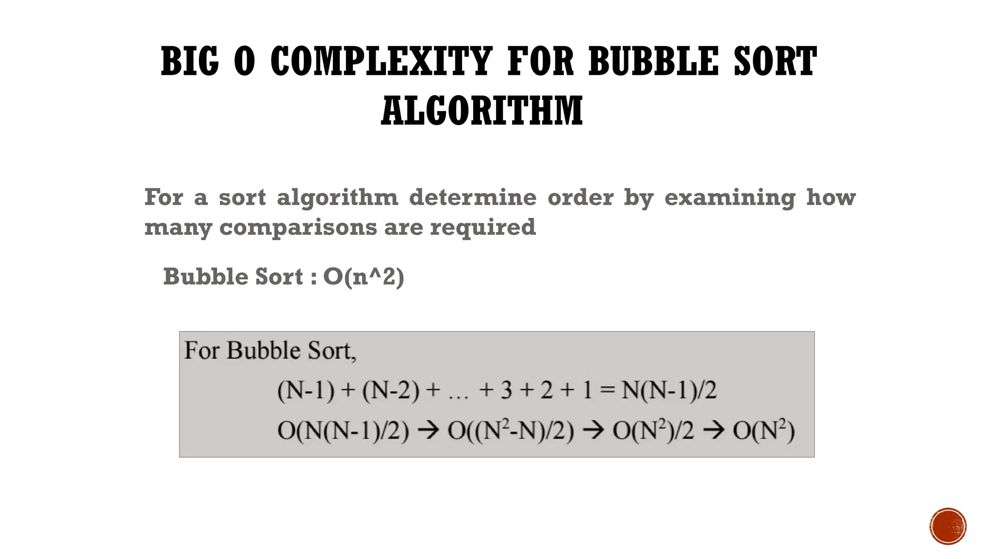
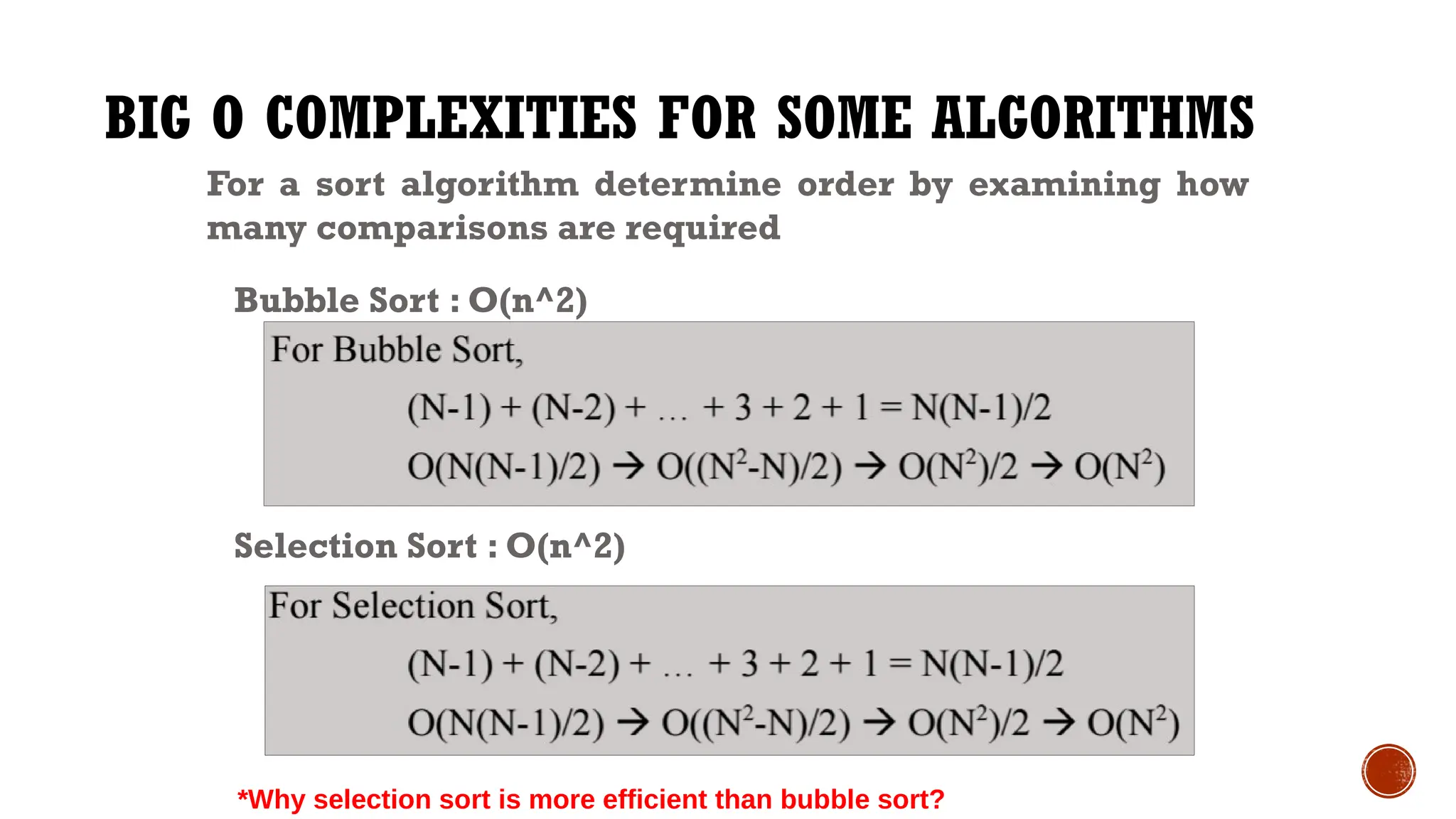
BIG O COMPLEXITYFOR BUBBLE SORT
ALGORITHM
For a sort algorithm determine order by examining how
many comparisons are required
Bubble Sort : O(n^2)
11.
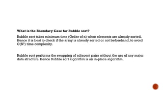
What is theBoundary Case for Bubble sort?
Bubble sort takes minimum time (Order of n) when elements are already sorted.
Hence it is best to check if the array is already sorted or not beforehand, to avoid
O(N2
) time complexity.
Bubble sort performs the swapping of adjacent pairs without the use of any major
data structure. Hence Bubble sort algorithm is an in-place algorithm.
12.
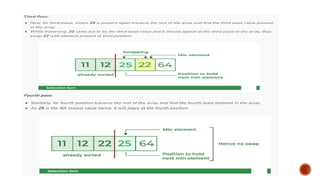
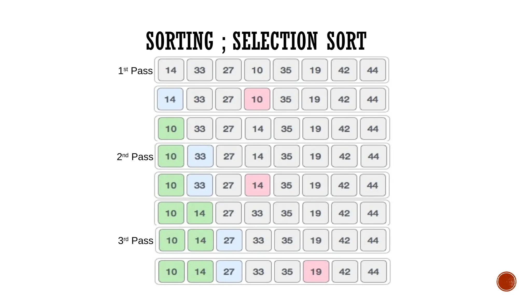
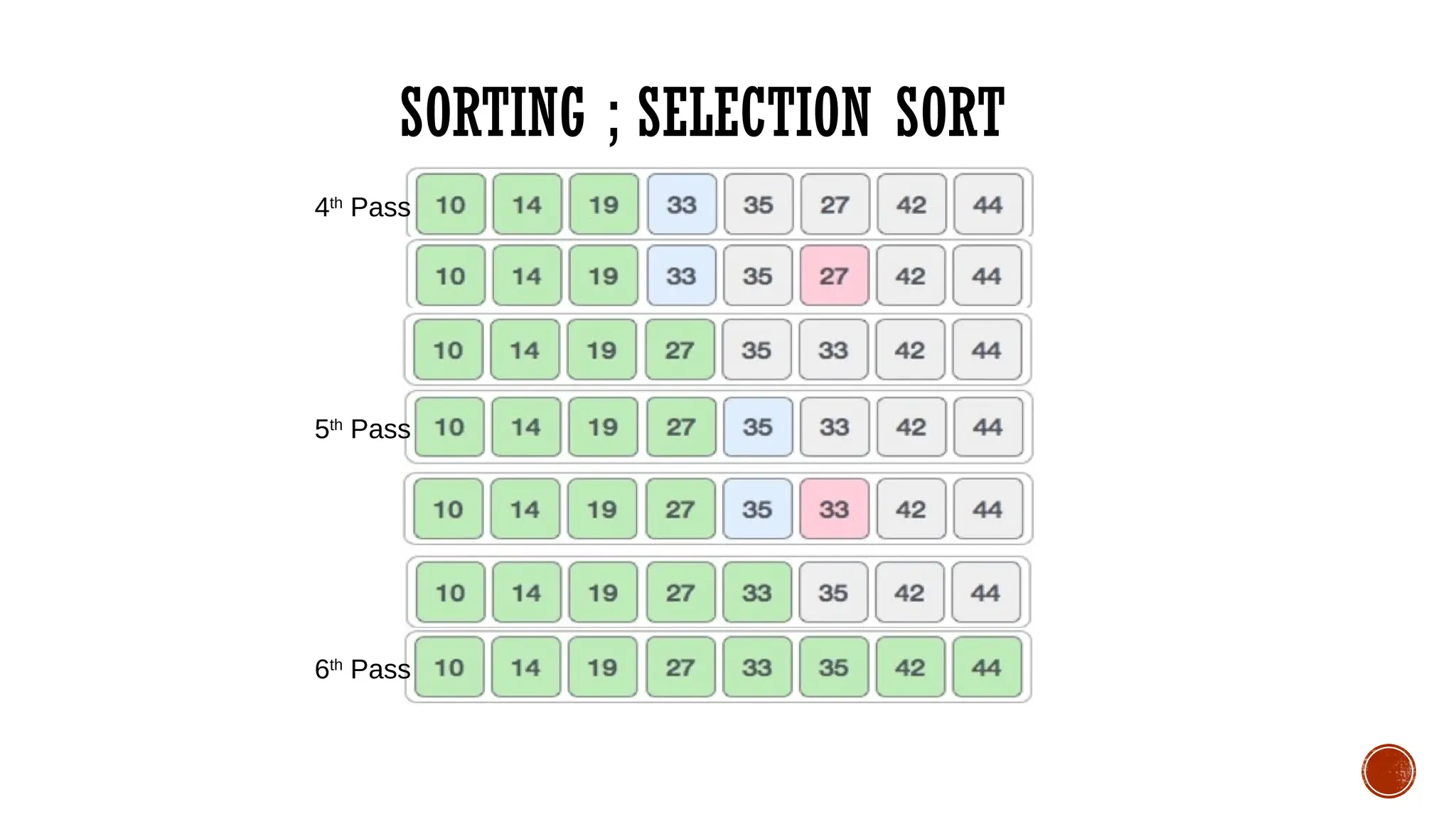
SELECTION SORT
Selection sortis a simple and efficient sorting algorithm that works by repeatedly
selecting the smallest (or largest) element from the unsorted portion of the list and
moving it to the sorted portion of the list.
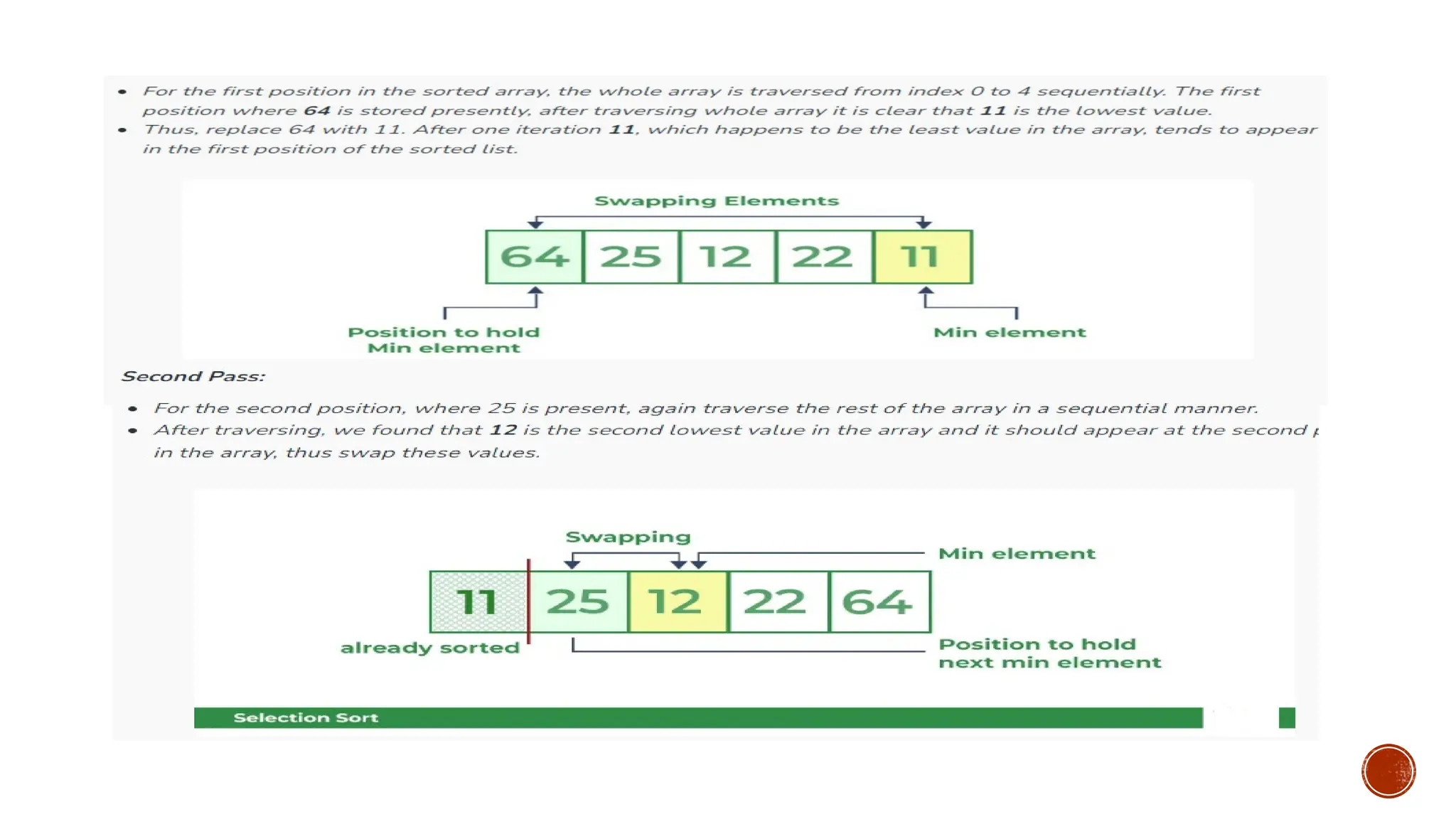
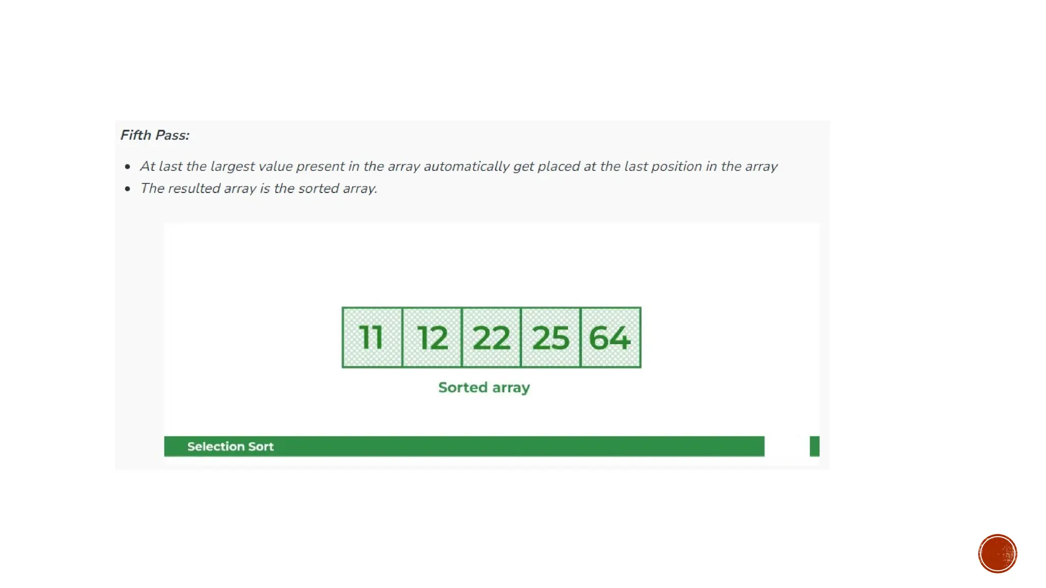
Lets consider the following array as an example:
arr[] = {64, 25, 12, 22, 11}
SORTING ; SELECTIONSORT
Algorithm: (Selection Sort) SELECTION (DATA,N)
Here DATA is a array with N elements.This
algorithm sorts the elements in DATA.
1. Repeat for I = 0 to N-2.
2. Set MIN=I
3. Repeat for J=I+1 to N-1.
4. If DATA[J] < DATA[MIN] then,
Set MIN=J.
[End of IF structure]
[End of inner loop]
Interchange DATA[I] and DATA[MIN].
[End of Step 1 outer loop]
4. Exit.
19.
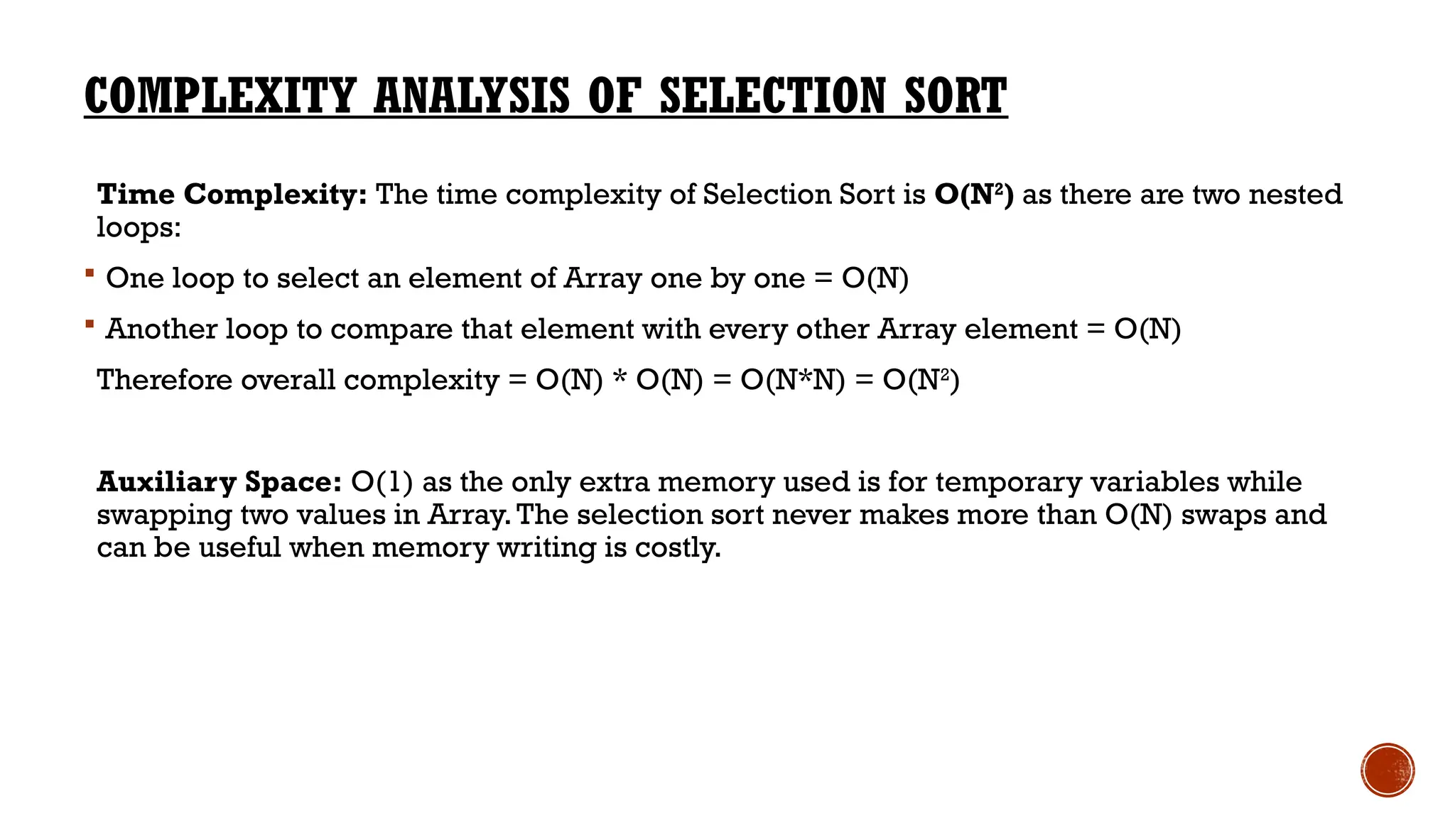
COMPLEXITY ANALYSIS OFSELECTION SORT
Time Complexity: The time complexity of Selection Sort is O(N2
) as there are two nested
loops:
One loop to select an element of Array one by one = O(N)
Another loop to compare that element with every other Array element = O(N)
Therefore overall complexity = O(N) * O(N) = O(N*N) = O(N2
)
Auxiliary Space: O(1) as the only extra memory used is for temporary variables while
swapping two values in Array.The selection sort never makes more than O(N) swaps and
can be useful when memory writing is costly.
20.
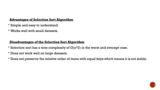
Advantages of SelectionSort Algorithm
Simple and easy to understand.
Works well with small datasets.
Disadvantages of the Selection Sort Algorithm
Selection sort has a time complexity of O(n^2) in the worst and average case.
Does not work well on large datasets.
Does not preserve the relative order of items with equal keys which means it is not stable.
21.
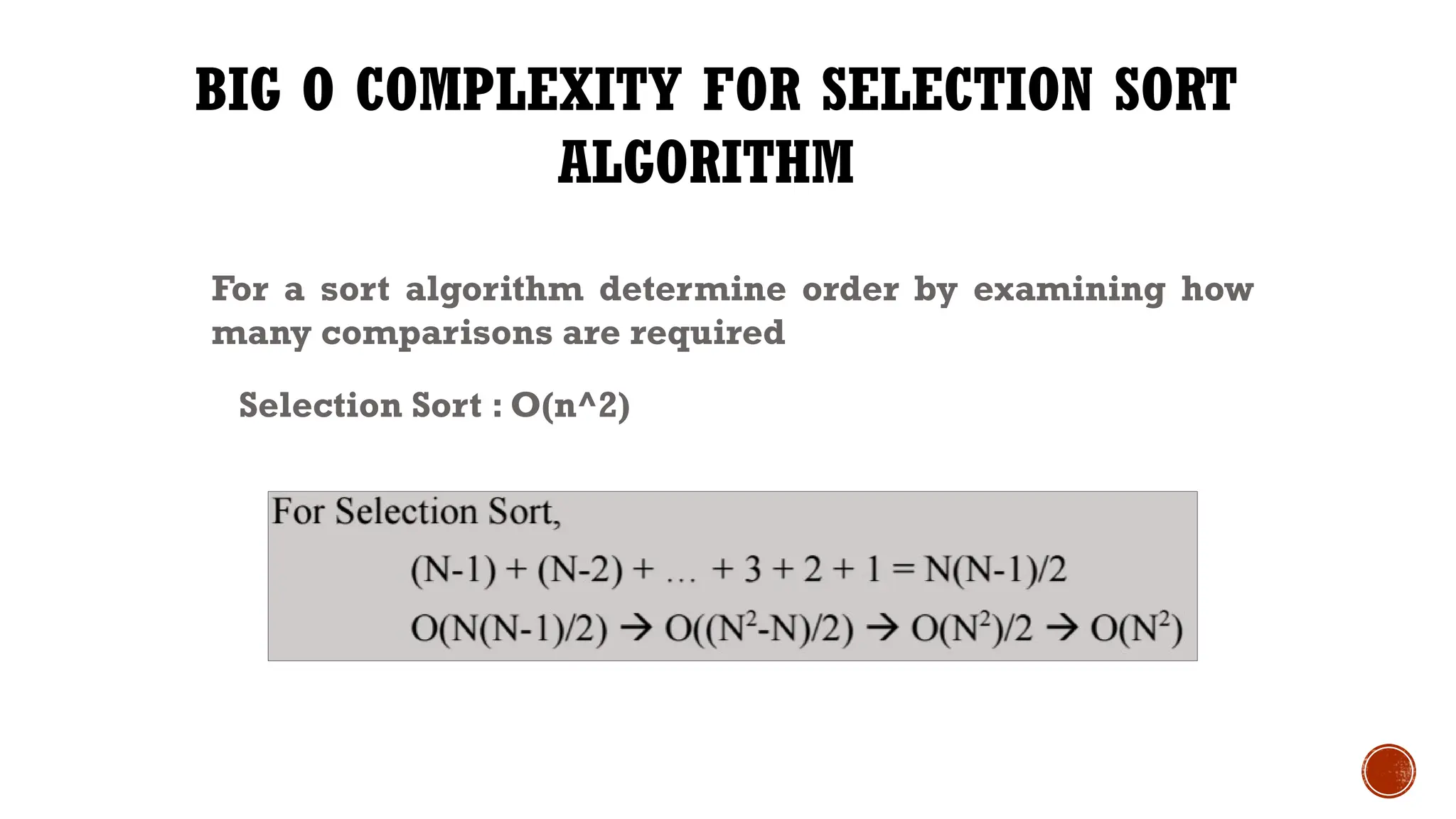
BIG O COMPLEXITYFOR SELECTION SORT
ALGORITHM
For a sort algorithm determine order by examining how
many comparisons are required
Selection Sort : O(n^2)
22.
BIG O COMPLEXITIESFOR SOME ALGORITHMS
For a sort algorithm determine order by examining how
many comparisons are required
Bubble Sort : O(n^2)
Selection Sort : O(n^2)
*Why selection sort is more efficient than bubble sort?
23.
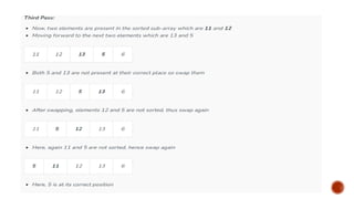
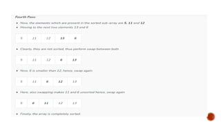
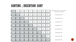
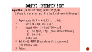
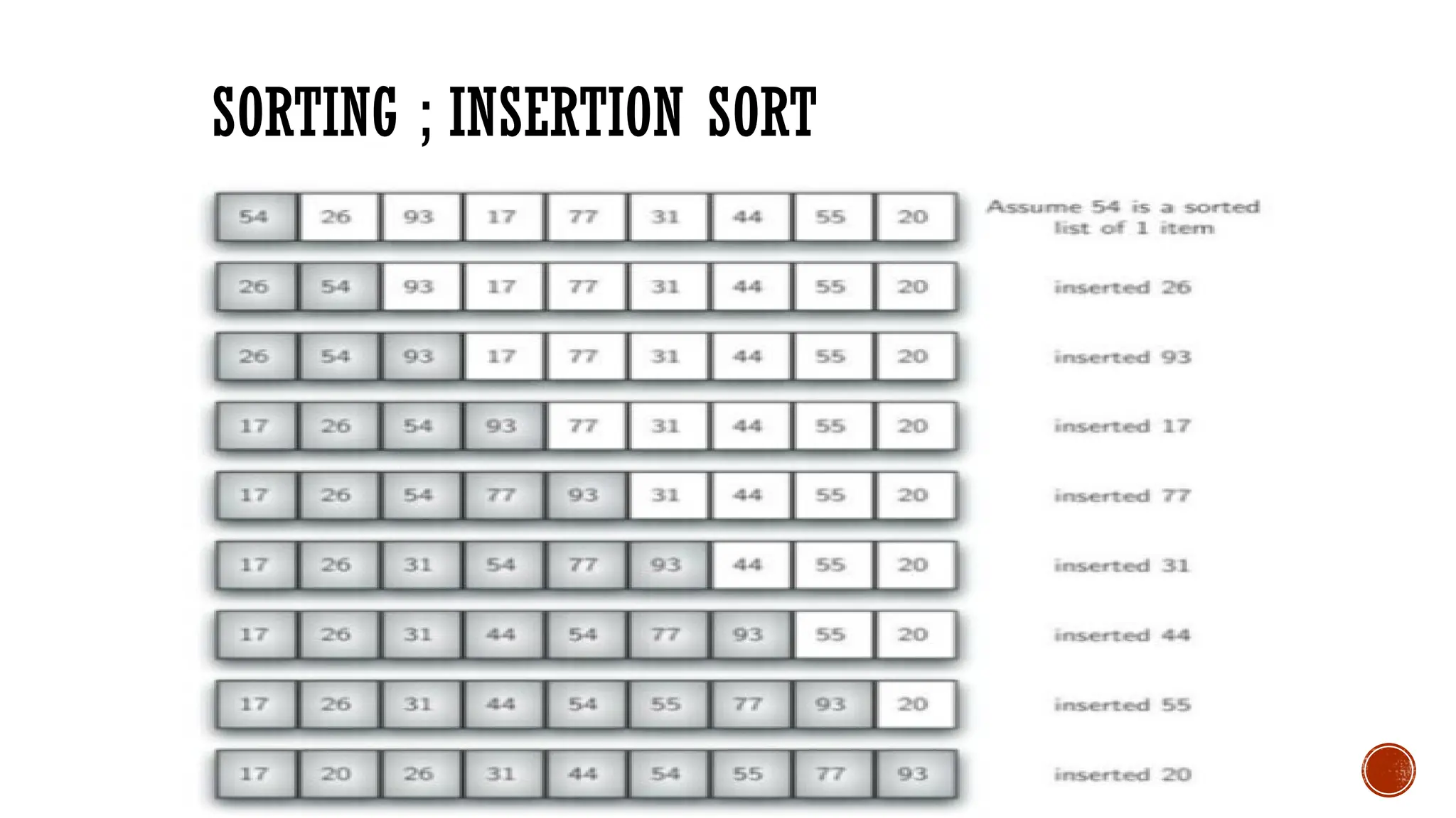
INSERTION SORT
Insertion sortis a simple sorting algorithm that works similar to the way you sort playing
cards in your hands.The array is virtually split into a sorted and an unsorted part.Values from
the unsorted part are picked and placed at the correct position in the sorted part.
To sort an array of size N in ascending order iterate over the array and compare the current
element (key) to its predecessor,if the key element is smaller than its predecessor, compare it
to the elements before.Move the greater elements one position up to make space for the
swapped element.
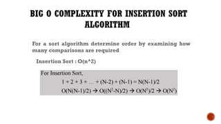
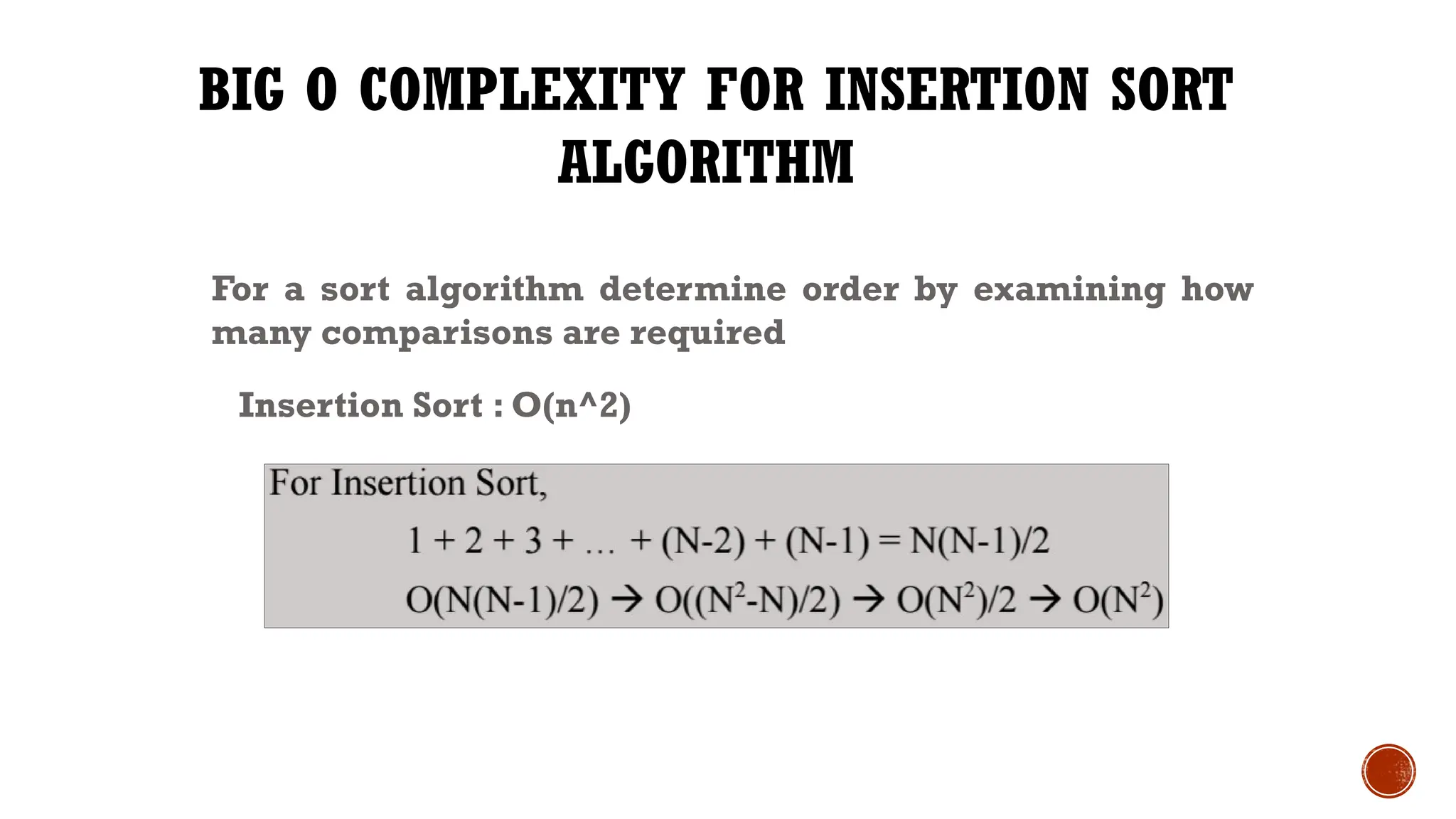
BIG O COMPLEXITYFOR INSERTION SORT
ALGORITHM
For a sort algorithm determine order by examining how
many comparisons are required
Insertion Sort : O(n^2)
30.
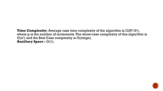
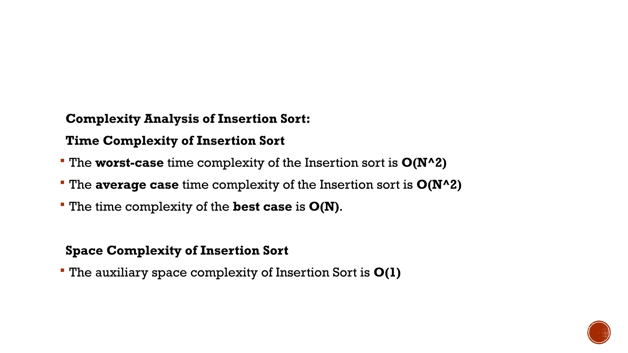
Complexity Analysis ofInsertion Sort:
Time Complexity of Insertion Sort
The worst-case time complexity of the Insertion sort is O(N^2)
The average case time complexity of the Insertion sort is O(N^2)
The time complexity of the best case is O(N).
Space Complexity of Insertion Sort
The auxiliary space complexity of Insertion Sort is O(1)
31.
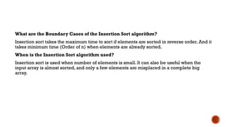
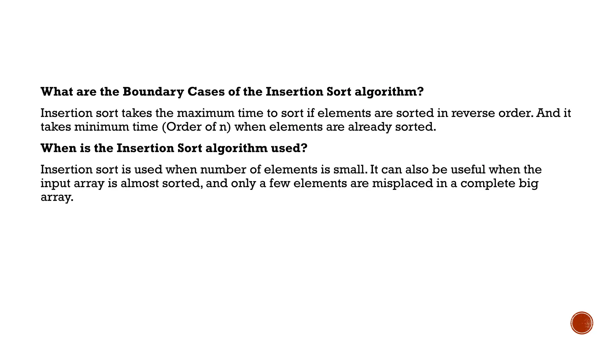
What are theBoundary Cases of the Insertion Sort algorithm?
Insertion sort takes the maximum time to sort if elements are sorted in reverse order. And it
takes minimum time (Order of n) when elements are already sorted.
When is the Insertion Sort algorithm used?
Insertion sort is used when number of elements is small. It can also be useful when the
input array is almost sorted, and only a few elements are misplaced in a complete big
array.
32.
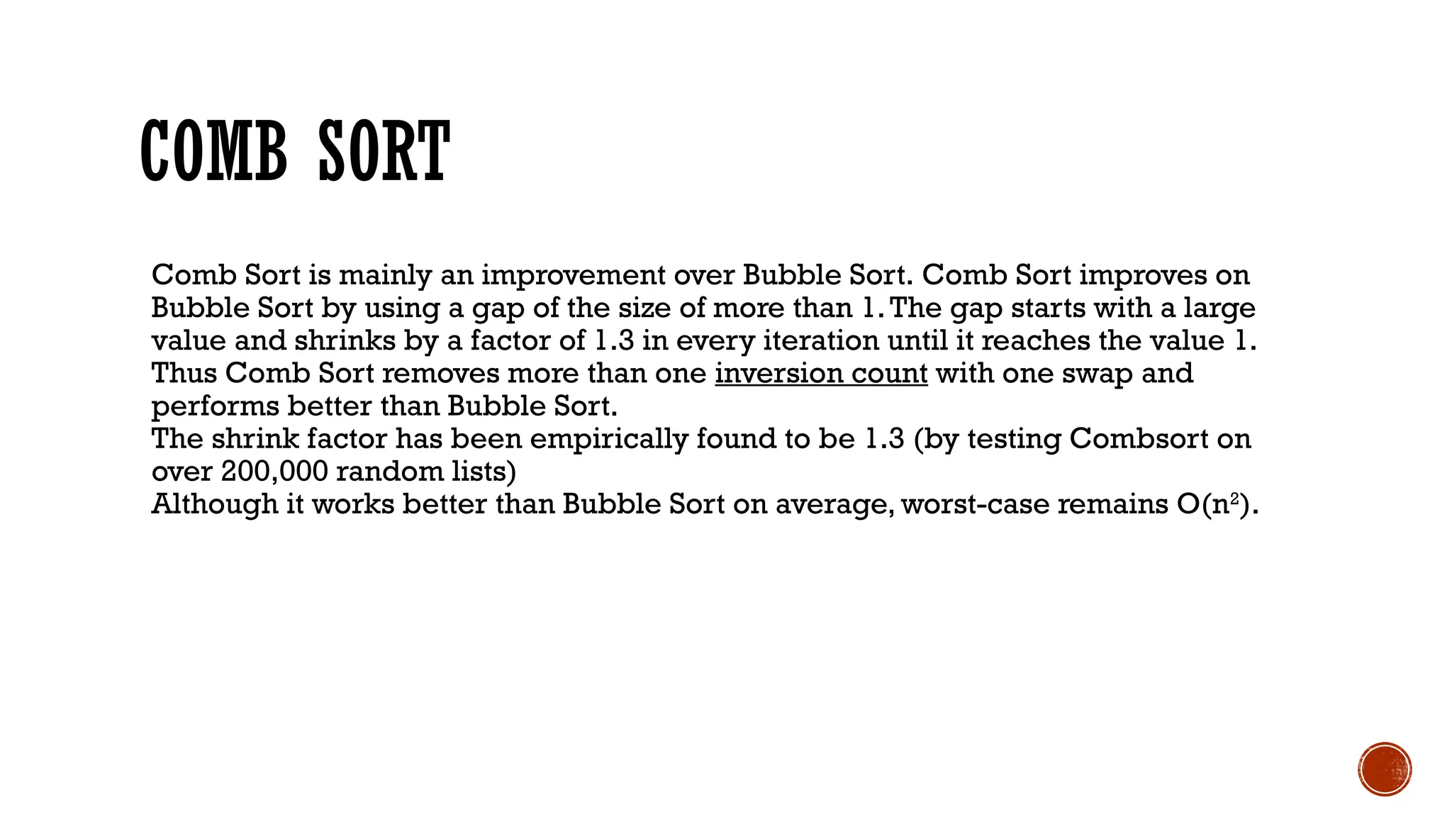
COMB SORT
Comb Sortis mainly an improvement over Bubble Sort. Comb Sort improves on
Bubble Sort by using a gap of the size of more than 1.The gap starts with a large
value and shrinks by a factor of 1.3 in every iteration until it reaches the value 1.
Thus Comb Sort removes more than one inversion count with one swap and
performs better than Bubble Sort.
The shrink factor has been empirically found to be 1.3 (by testing Combsort on
over 200,000 random lists)
Although it works better than Bubble Sort on average, worst-case remains O(n2
).
33.
combSort(arr, n):
gap =n
shrink = 1.3
swapped = true
while (gap > 1 or swapped):
gap = floor(gap / shrink)
if gap < 1:
gap = 1
swapped = false
for i = 0 to n - gap - 1:
if arr[i] > arr[i + gap]:
swap(arr[i], arr[i + gap])
swapped = true
34.
Example Dry Run
Array:[8, 4, 1, 56, 3, -44, 23]
Initial gap = 7 shrink 5
→ →
Compare (arr[0], arr[5]) swap [ -44, 4, 1, 56, 3, 8, 23 ]
→ →
Gap = 3 compare and swap elements 3 apart
→
Gap = 2 compare elements 2 apart
→
Gap = 1 now it works like Bubble Sort until fully sorted.
→
Final Sorted: [-44, 1, 3, 4, 8, 23, 56]
35.
Time Complexity: Averagecase time complexity of the algorithm is (N
Ω 2
/2p
),
where p is the number of increments.The worst-case complexity of this algorithm is
O(n2
) and the Best Case complexity is O(nlogn).
Auxiliary Space : O(1).
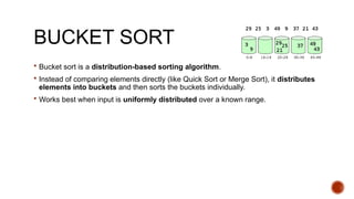
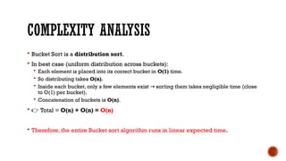
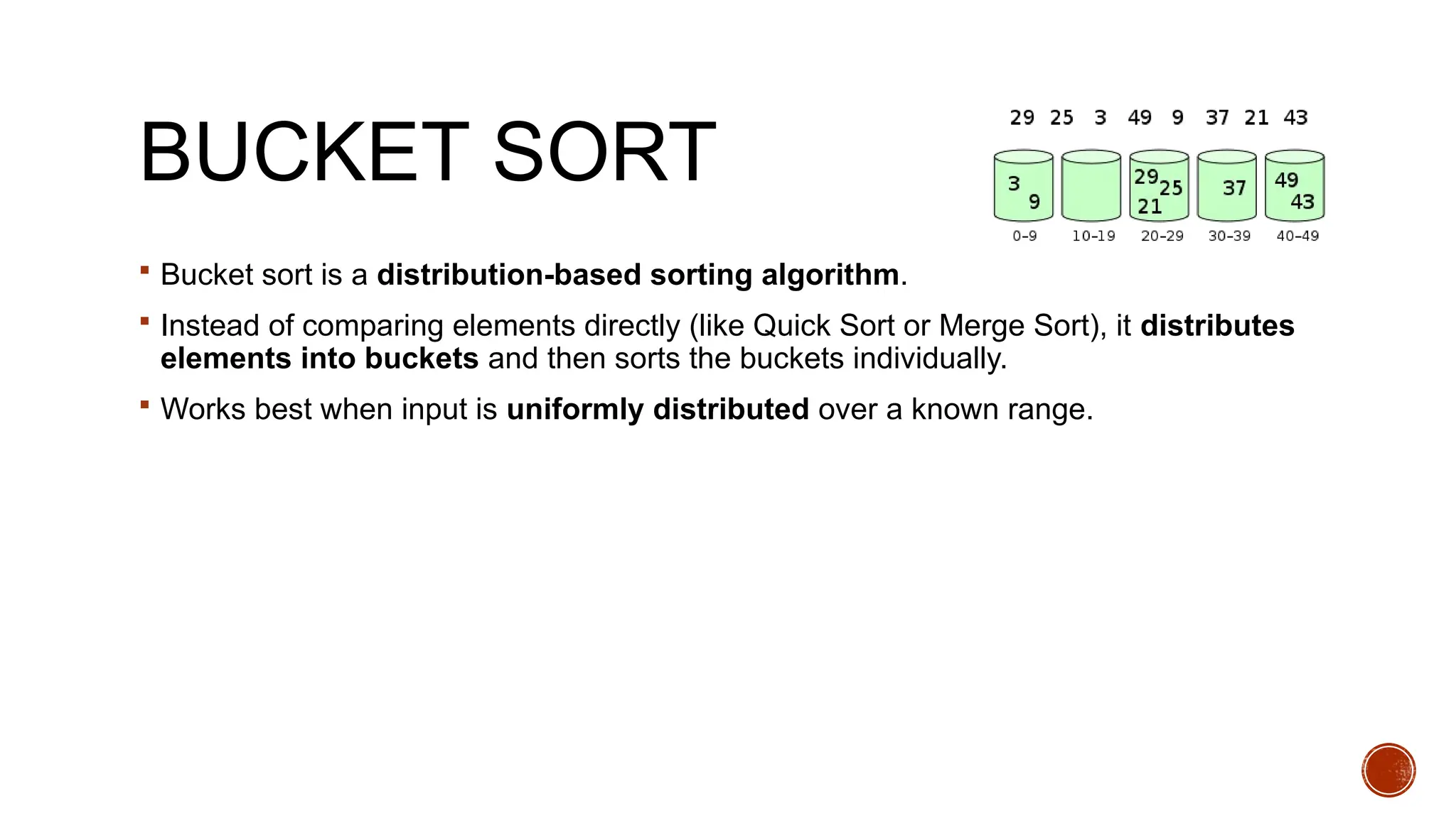
BUCKET SORT
Bucketsort is a distribution-based sorting algorithm.
Instead of comparing elements directly (like Quick Sort or Merge Sort), it distributes
elements into buckets and then sorts the buckets individually.
Works best when input is uniformly distributed over a known range.
38.
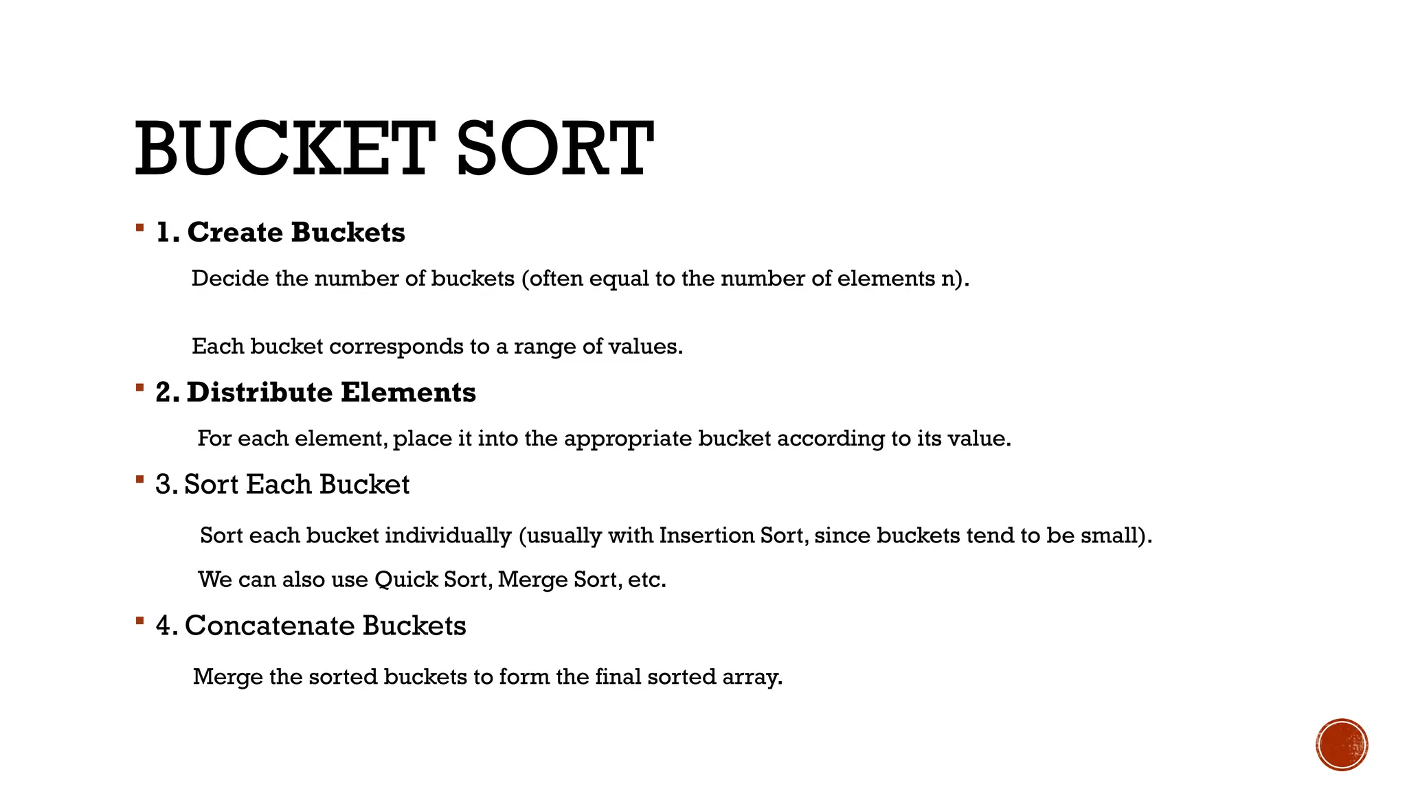
BUCKET SORT
1.Create Buckets
Decide the number of buckets (often equal to the number of elements n).
Each bucket corresponds to a range of values.
2. Distribute Elements
For each element, place it into the appropriate bucket according to its value.
3. Sort Each Bucket
Sort each bucket individually (usually with Insertion Sort, since buckets tend to be small).
We can also use Quick Sort, Merge Sort, etc.
4. Concatenate Buckets
Merge the sorted buckets to form the final sorted array.
39.
To convertnormal numbers into [0,1) range for bucket sort:
x
Array: [25, 50, 75, 100]
min = 25, max = 100
Convert each number:
25 (25-25)/(100-25) = 0/75 = 0
→
50 (50-25)/75 = 25/75 = 0.33
→
75 (75-25)/75 = 50/75 = 0.67
→
100 (100-25)/75 = 75/75 = 1
→
Now array becomes: [0, 0.33, 0.67, 1] perfect for bucket sort.
→
40.
PSEUDOCODE
bucketSort(arr, n):
create nempty buckets
for i = 0 to n-1:
index = floor(n * arr[i]) // assuming 0 <= arr[i] < 1
insert arr[i] into bucket[index]
for each bucket:
sort(bucket) // insertion sort or other algorithm
concatenate all buckets
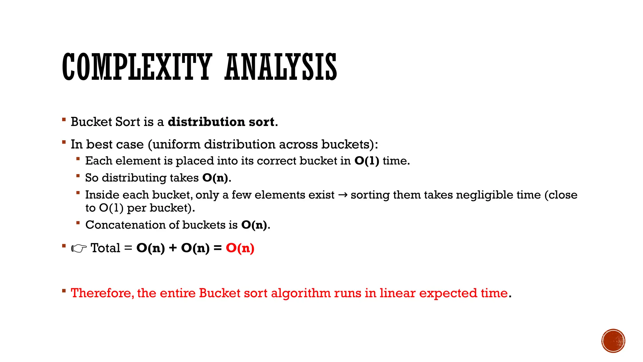
COMPLEXITY ANALYSIS
BucketSort is a distribution sort.
In best case (uniform distribution across buckets):
Each element is placed into its correct bucket in O(1) time.
So distributing takes O(n).
Inside each bucket, only a few elements exist sorting them takes negligible time (close
→
to O(1) per bucket).
Concatenation of buckets is O(n).
👉 Total = O(n) + O(n) = O(n)
Therefore, the entire Bucket sort algorithm runs in linear expected time.
43.
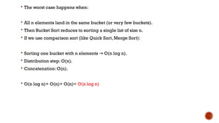
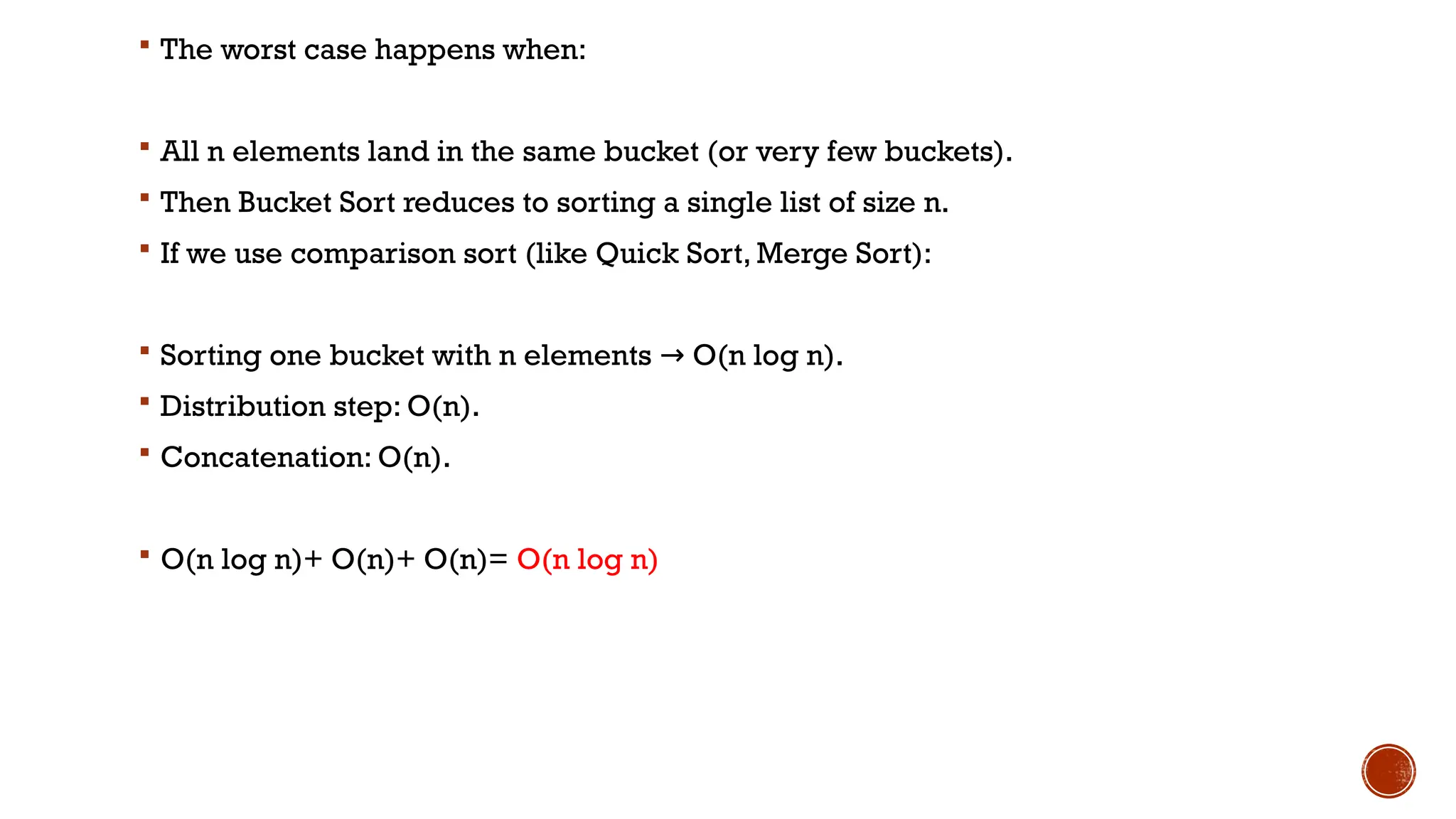
The worstcase happens when:
All n elements land in the same bucket (or very few buckets).
Then Bucket Sort reduces to sorting a single list of size n.
If we use comparison sort (like Quick Sort, Merge Sort):
Sorting one bucket with n elements O(n log n).
→
Distribution step: O(n).
Concatenation: O(n).
O(n log n)+ O(n)+ O(n)= O(n log n)
44.
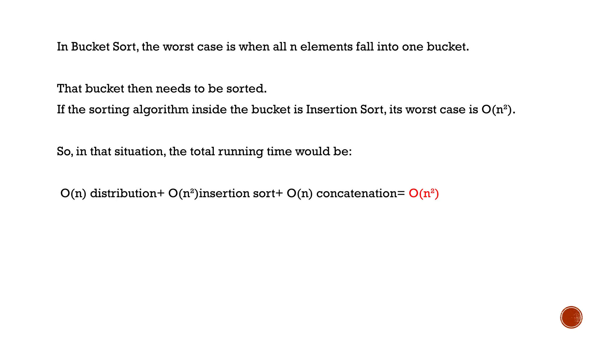
In Bucket Sort,the worst case is when all n elements fall into one bucket.
That bucket then needs to be sorted.
If the sorting algorithm inside the bucket is Insertion Sort, its worst case is O(n²).
So, in that situation, the total running time would be:
O(n) distribution+ O(n²)insertion sort+ O(n) concatenation= O(n²)
45.
RADIX SORT
RadixSort is a non-comparison-based sorting algorithm.
It works by sorting numbers digit by digit, starting either from the least significant
digit (LSD) or the most significant digit (MSD).
It uses a stable sorting algorithm (often Counting Sort) as a subroutine to sort
digits.
46.
HOW RADIX SORTWORKS (LSD VERSION)
Example: Sort [170, 45, 75, 90, 802, 24, 2, 66]
Find the maximum number 802 (3 digits).
→
→ So, we need 3 passes (for units, tens, hundreds).
Sort by least significant digit (1’s place):
[170, 90, 802, 2, 24, 45, 75, 66]
Sort by 10’s place:
[802, 2, 24, 45, 66, 170, 75, 90]
Sort by 100’s place:
[2, 24, 45, 66, 75, 90, 170, 802]
47.
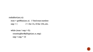
radixSort(arr, n):
max =getMax(arr, n) // find max number
exp = 1 // 1 for 1’s, 10 for 10’s, etc.
while (max / exp > 0):
countingSortByDigit(arr, n, exp)
exp = exp * 10
48.
void countingSortByDigit(int arr[],int n,
int exp) {
int output[n]; // output array
(sorted by digit)
int count[10] = {0}; // count array for
digits 0–9 (base 10)
// Step 1: Count occurrences of digits
for (int i = 0; i < n; i++) {
int digit = (arr[i] / exp) % 10;
count[digit]++;
}
// Step 2: Update count[] to store
cumulative positions
for (int i = 1; i < 10; i++) {
count[i] += count[i - 1];
}
// Step 3: Build output[] (iterate from right to left
to ensure stability)
for (int i = n - 1; i >= 0; i--) {
int digit = (arr[i] / exp) % 10;
output[count[digit] - 1] = arr[i];
count[digit]--;
}
// Step 4: Copy output[] back to arr[]
for (int i = 0; i < n; i++) {
arr[i] = output[i];
}
}


![HOW DOES BUBBLE SORT WORK?
Input: arr[] = {6,0,3,5}](https://image.slidesharecdn.com/fall2025-sortinglectures-251014042106-a7289fcf/85/Design-and-analysis-Sorting-Lectures-pptx-4-320.jpg)
![SORTING ; BUBBLE SORT
Algorithm: (Bubble Sort) BUBBLE(DATA,N)
Here DATA is a array with N elements.This
algorithm sorts the elements in DATA.
1. Repeat for PASS = 1 to N-1.
2. Repeat for i=0 to N-PASS.
3. If DATA[i] > DATA[i+1] then,
Interchange DATA[i] and DATA[i+1]
[End of IF structure]
[End of inner loop]
[End of Step 1 outer loop]
4. Exit.](https://image.slidesharecdn.com/fall2025-sortinglectures-251014042106-a7289fcf/85/Design-and-analysis-Sorting-Lectures-pptx-7-320.jpg)

![SELECTION SORT
Selection sort is a simple and efficient sorting algorithm that works by repeatedly
selecting the smallest (or largest) element from the unsorted portion of the list and
moving it to the sorted portion of the list.
Lets consider the following array as an example:
arr[] = {64, 25, 12, 22, 11}](https://image.slidesharecdn.com/fall2025-sortinglectures-251014042106-a7289fcf/85/Design-and-analysis-Sorting-Lectures-pptx-12-320.jpg)


![SORTING ; SELECTION SORT
Algorithm: (Selection Sort) SELECTION (DATA,N)
Here DATA is a array with N elements.This
algorithm sorts the elements in DATA.
1. Repeat for I = 0 to N-2.
2. Set MIN=I
3. Repeat for J=I+1 to N-1.
4. If DATA[J] < DATA[MIN] then,
Set MIN=J.
[End of IF structure]
[End of inner loop]
Interchange DATA[I] and DATA[MIN].
[End of Step 1 outer loop]
4. Exit.](https://image.slidesharecdn.com/fall2025-sortinglectures-251014042106-a7289fcf/85/Design-and-analysis-Sorting-Lectures-pptx-18-320.jpg)


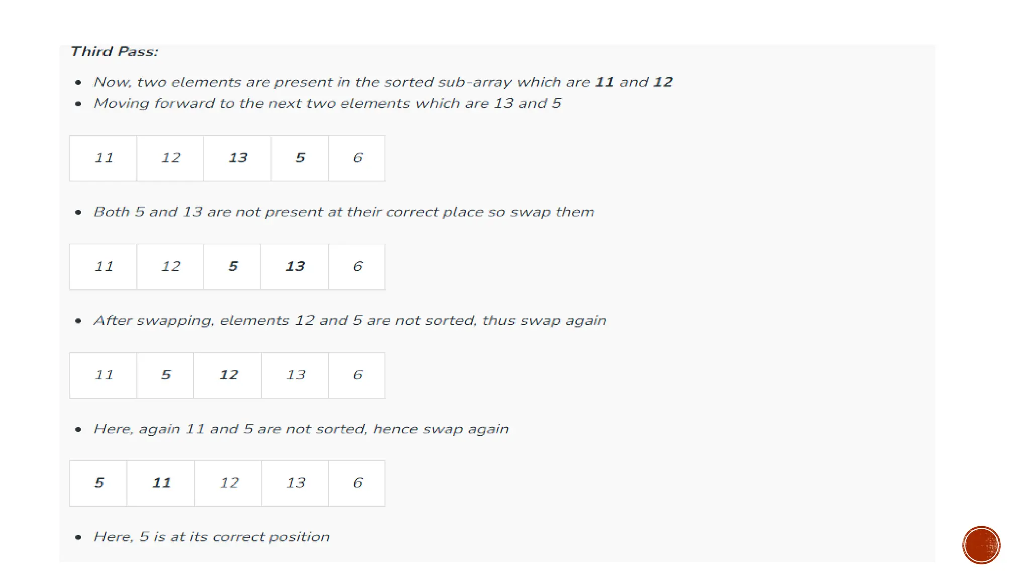
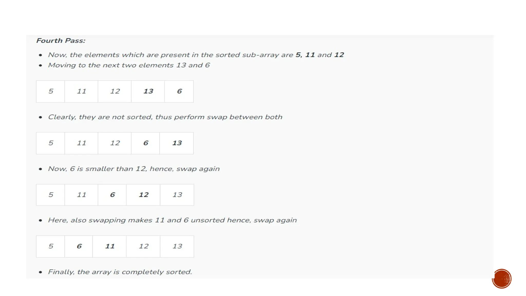
![Consider an example: arr[]: {12, 11, 13, 5, 6}](https://image.slidesharecdn.com/fall2025-sortinglectures-251014042106-a7289fcf/85/Design-and-analysis-Sorting-Lectures-pptx-24-320.jpg)


![combSort(arr, n):
gap = n
shrink = 1.3
swapped = true
while (gap > 1 or swapped):
gap = floor(gap / shrink)
if gap < 1:
gap = 1
swapped = false
for i = 0 to n - gap - 1:
if arr[i] > arr[i + gap]:
swap(arr[i], arr[i + gap])
swapped = true](https://image.slidesharecdn.com/fall2025-sortinglectures-251014042106-a7289fcf/85/Design-and-analysis-Sorting-Lectures-pptx-33-320.jpg)
![Example Dry Run
Array: [8, 4, 1, 56, 3, -44, 23]
Initial gap = 7 shrink 5
→ →
Compare (arr[0], arr[5]) swap [ -44, 4, 1, 56, 3, 8, 23 ]
→ →
Gap = 3 compare and swap elements 3 apart
→
Gap = 2 compare elements 2 apart
→
Gap = 1 now it works like Bubble Sort until fully sorted.
→
Final Sorted: [-44, 1, 3, 4, 8, 23, 56]](https://image.slidesharecdn.com/fall2025-sortinglectures-251014042106-a7289fcf/85/Design-and-analysis-Sorting-Lectures-pptx-34-320.jpg)


![ To convert normal numbers into [0,1) range for bucket sort:
x
Array: [25, 50, 75, 100]
min = 25, max = 100
Convert each number:
25 (25-25)/(100-25) = 0/75 = 0
→
50 (50-25)/75 = 25/75 = 0.33
→
75 (75-25)/75 = 50/75 = 0.67
→
100 (100-25)/75 = 75/75 = 1
→
Now array becomes: [0, 0.33, 0.67, 1] perfect for bucket sort.
→](https://image.slidesharecdn.com/fall2025-sortinglectures-251014042106-a7289fcf/85/Design-and-analysis-Sorting-Lectures-pptx-39-320.jpg)
![PSEUDOCODE
bucketSort(arr, n):
create n empty buckets
for i = 0 to n-1:
index = floor(n * arr[i]) // assuming 0 <= arr[i] < 1
insert arr[i] into bucket[index]
for each bucket:
sort(bucket) // insertion sort or other algorithm
concatenate all buckets](https://image.slidesharecdn.com/fall2025-sortinglectures-251014042106-a7289fcf/85/Design-and-analysis-Sorting-Lectures-pptx-40-320.jpg)
![EXAMPLE
[0.78, 0.17, 0.39, 0.26, 0.72, 0.94, 0.21, 0.12, 0.23, 0.68]
1. Create 10 buckets (B0 … B9).
2. Distribute elements:
B1: [0.17, 0.12]
B2: [0.26, 0.21, 0.23]
B3: [0.39]
B6: [0.68]
B7: [0.78, 0.72]
B9: [0.94]
3. Sort each bucket:
B1: [0.12, 0.17]
B2: [0.21, 0.23, 0.26]
B7: [0.72, 0.78]
4. Concatenate buckets:
[0.12, 0.17, 0.21, 0.23, 0.26, 0.39, 0.68, 0.72, 0.78, 0.94]](https://image.slidesharecdn.com/fall2025-sortinglectures-251014042106-a7289fcf/85/Design-and-analysis-Sorting-Lectures-pptx-41-320.jpg)


![HOW RADIX SORT WORKS (LSD VERSION)
Example: Sort [170, 45, 75, 90, 802, 24, 2, 66]
Find the maximum number 802 (3 digits).
→
→ So, we need 3 passes (for units, tens, hundreds).
Sort by least significant digit (1’s place):
[170, 90, 802, 2, 24, 45, 75, 66]
Sort by 10’s place:
[802, 2, 24, 45, 66, 170, 75, 90]
Sort by 100’s place:
[2, 24, 45, 66, 75, 90, 170, 802]](https://image.slidesharecdn.com/fall2025-sortinglectures-251014042106-a7289fcf/85/Design-and-analysis-Sorting-Lectures-pptx-46-320.jpg)
![void countingSortByDigit(int arr[], int n,
int exp) {
int output[n]; // output array
(sorted by digit)
int count[10] = {0}; // count array for
digits 0–9 (base 10)
// Step 1: Count occurrences of digits
for (int i = 0; i < n; i++) {
int digit = (arr[i] / exp) % 10;
count[digit]++;
}
// Step 2: Update count[] to store
cumulative positions
for (int i = 1; i < 10; i++) {
count[i] += count[i - 1];
}
// Step 3: Build output[] (iterate from right to left
to ensure stability)
for (int i = n - 1; i >= 0; i--) {
int digit = (arr[i] / exp) % 10;
output[count[digit] - 1] = arr[i];
count[digit]--;
}
// Step 4: Copy output[] back to arr[]
for (int i = 0; i < n; i++) {
arr[i] = output[i];
}
}](https://image.slidesharecdn.com/fall2025-sortinglectures-251014042106-a7289fcf/85/Design-and-analysis-Sorting-Lectures-pptx-48-320.jpg)


![HOW DOES BUBBLE SORT WORK?
Input: arr[] = {6,0,3,5}](https://image.slidesharecdn.com/fall2025-sortinglectures-251014042106-a7289fcf/75/Design-and-analysis-Sorting-Lectures-pptx-4-2048.jpg)


![SORTING ; BUBBLE SORT
Algorithm: (Bubble Sort) BUBBLE(DATA,N)
Here DATA is a array with N elements.This
algorithm sorts the elements in DATA.
1. Repeat for PASS = 1 to N-1.
2. Repeat for i=0 to N-PASS.
3. If DATA[i] > DATA[i+1] then,
Interchange DATA[i] and DATA[i+1]
[End of IF structure]
[End of inner loop]
[End of Step 1 outer loop]
4. Exit.](https://image.slidesharecdn.com/fall2025-sortinglectures-251014042106-a7289fcf/75/Design-and-analysis-Sorting-Lectures-pptx-7-2048.jpg)

![SELECTION SORT
Selection sort is a simple and efficient sorting algorithm that works by repeatedly
selecting the smallest (or largest) element from the unsorted portion of the list and
moving it to the sorted portion of the list.
Lets consider the following array as an example:
arr[] = {64, 25, 12, 22, 11}](https://image.slidesharecdn.com/fall2025-sortinglectures-251014042106-a7289fcf/75/Design-and-analysis-Sorting-Lectures-pptx-12-2048.jpg)

![SORTING ; SELECTION SORT
Algorithm: (Selection Sort) SELECTION (DATA,N)
Here DATA is a array with N elements.This
algorithm sorts the elements in DATA.
1. Repeat for I = 0 to N-2.
2. Set MIN=I
3. Repeat for J=I+1 to N-1.
4. If DATA[J] < DATA[MIN] then,
Set MIN=J.
[End of IF structure]
[End of inner loop]
Interchange DATA[I] and DATA[MIN].
[End of Step 1 outer loop]
4. Exit.](https://image.slidesharecdn.com/fall2025-sortinglectures-251014042106-a7289fcf/75/Design-and-analysis-Sorting-Lectures-pptx-18-2048.jpg)

![Consider an example: arr[]: {12, 11, 13, 5, 6}](https://image.slidesharecdn.com/fall2025-sortinglectures-251014042106-a7289fcf/75/Design-and-analysis-Sorting-Lectures-pptx-24-2048.jpg)
![combSort(arr, n):
gap = n
shrink = 1.3
swapped = true
while (gap > 1 or swapped):
gap = floor(gap / shrink)
if gap < 1:
gap = 1
swapped = false
for i = 0 to n - gap - 1:
if arr[i] > arr[i + gap]:
swap(arr[i], arr[i + gap])
swapped = true](https://image.slidesharecdn.com/fall2025-sortinglectures-251014042106-a7289fcf/75/Design-and-analysis-Sorting-Lectures-pptx-33-2048.jpg)
![Example Dry Run
Array: [8, 4, 1, 56, 3, -44, 23]
Initial gap = 7 shrink 5
→ →
Compare (arr[0], arr[5]) swap [ -44, 4, 1, 56, 3, 8, 23 ]
→ →
Gap = 3 compare and swap elements 3 apart
→
Gap = 2 compare elements 2 apart
→
Gap = 1 now it works like Bubble Sort until fully sorted.
→
Final Sorted: [-44, 1, 3, 4, 8, 23, 56]](https://image.slidesharecdn.com/fall2025-sortinglectures-251014042106-a7289fcf/75/Design-and-analysis-Sorting-Lectures-pptx-34-2048.jpg)

![ To convert normal numbers into [0,1) range for bucket sort:
x
Array: [25, 50, 75, 100]
min = 25, max = 100
Convert each number:
25 (25-25)/(100-25) = 0/75 = 0
→
50 (50-25)/75 = 25/75 = 0.33
→
75 (75-25)/75 = 50/75 = 0.67
→
100 (100-25)/75 = 75/75 = 1
→
Now array becomes: [0, 0.33, 0.67, 1] perfect for bucket sort.
→](https://image.slidesharecdn.com/fall2025-sortinglectures-251014042106-a7289fcf/75/Design-and-analysis-Sorting-Lectures-pptx-39-2048.jpg)
![PSEUDOCODE
bucketSort(arr, n):
create n empty buckets
for i = 0 to n-1:
index = floor(n * arr[i]) // assuming 0 <= arr[i] < 1
insert arr[i] into bucket[index]
for each bucket:
sort(bucket) // insertion sort or other algorithm
concatenate all buckets](https://image.slidesharecdn.com/fall2025-sortinglectures-251014042106-a7289fcf/75/Design-and-analysis-Sorting-Lectures-pptx-40-2048.jpg)
![EXAMPLE
[0.78, 0.17, 0.39, 0.26, 0.72, 0.94, 0.21, 0.12, 0.23, 0.68]
1. Create 10 buckets (B0 … B9).
2. Distribute elements:
B1: [0.17, 0.12]
B2: [0.26, 0.21, 0.23]
B3: [0.39]
B6: [0.68]
B7: [0.78, 0.72]
B9: [0.94]
3. Sort each bucket:
B1: [0.12, 0.17]
B2: [0.21, 0.23, 0.26]
B7: [0.72, 0.78]
4. Concatenate buckets:
[0.12, 0.17, 0.21, 0.23, 0.26, 0.39, 0.68, 0.72, 0.78, 0.94]](https://image.slidesharecdn.com/fall2025-sortinglectures-251014042106-a7289fcf/75/Design-and-analysis-Sorting-Lectures-pptx-41-2048.jpg)
![HOW RADIX SORT WORKS (LSD VERSION)
Example: Sort [170, 45, 75, 90, 802, 24, 2, 66]
Find the maximum number 802 (3 digits).
→
→ So, we need 3 passes (for units, tens, hundreds).
Sort by least significant digit (1’s place):
[170, 90, 802, 2, 24, 45, 75, 66]
Sort by 10’s place:
[802, 2, 24, 45, 66, 170, 75, 90]
Sort by 100’s place:
[2, 24, 45, 66, 75, 90, 170, 802]](https://image.slidesharecdn.com/fall2025-sortinglectures-251014042106-a7289fcf/75/Design-and-analysis-Sorting-Lectures-pptx-46-2048.jpg)

![void countingSortByDigit(int arr[], int n,
int exp) {
int output[n]; // output array
(sorted by digit)
int count[10] = {0}; // count array for
digits 0–9 (base 10)
// Step 1: Count occurrences of digits
for (int i = 0; i < n; i++) {
int digit = (arr[i] / exp) % 10;
count[digit]++;
}
// Step 2: Update count[] to store
cumulative positions
for (int i = 1; i < 10; i++) {
count[i] += count[i - 1];
}
// Step 3: Build output[] (iterate from right to left
to ensure stability)
for (int i = n - 1; i >= 0; i--) {
int digit = (arr[i] / exp) % 10;
output[count[digit] - 1] = arr[i];
count[digit]--;
}
// Step 4: Copy output[] back to arr[]
for (int i = 0; i < n; i++) {
arr[i] = output[i];
}
}](https://image.slidesharecdn.com/fall2025-sortinglectures-251014042106-a7289fcf/75/Design-and-analysis-Sorting-Lectures-pptx-48-2048.jpg)


![Agentic Systems and Compliance - A brief intro [1.2]](https://cdn.slidesharecdn.com/ss_thumbnails/agenticsystemsandcompliace-1-251018025303-958a42ec-thumbnail.jpg?width=600ounds&width=560&fit=bounds)


![RTP_AR_Basic_Learners' Workbook_KS2 [FOR REPRODUCTION] (1).pdf](https://cdn.slidesharecdn.com/ss_thumbnails/rtparbasiclearnersworkbookks2forreproduction1-251016024943-e51a16ac-thumbnail.jpg?width=600ounds&width=560&fit=bounds)