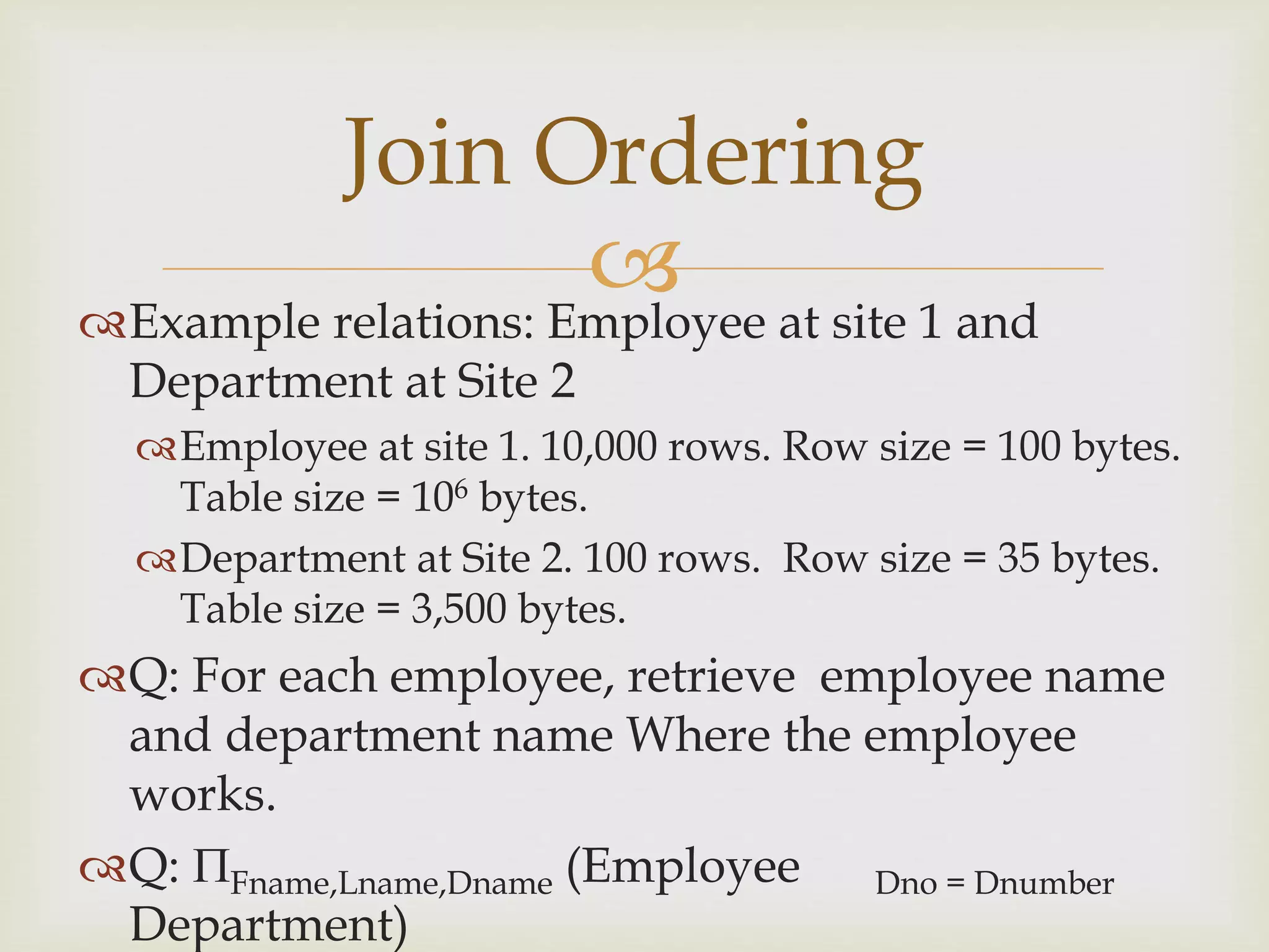
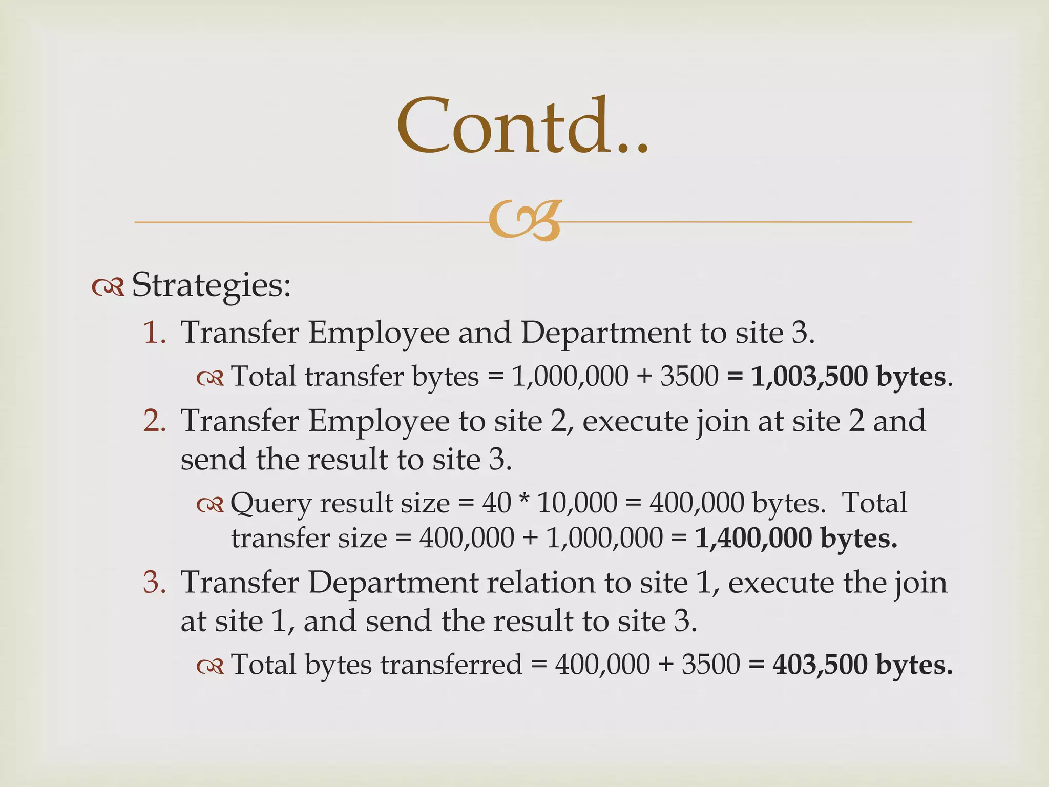
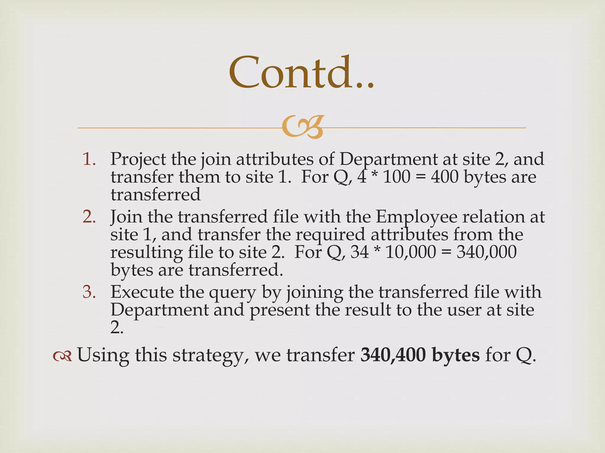
Downloaded 826 times


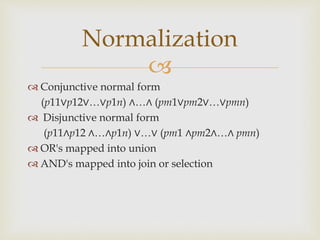
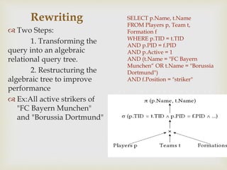

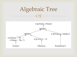
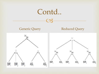
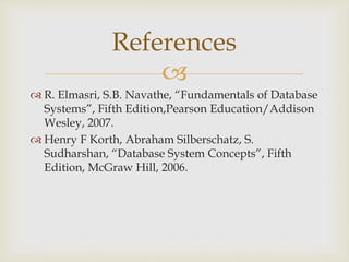
![
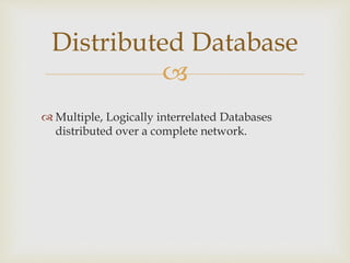
It is used to reduce the data transmission cost.
Computing steps:
1) Project Ri on attribute A (Ri[A] ) and
ship this projection ( a semijoin
projection) from the site of Ri to the site
of Rj ;
2) Reduce Rj to Rj’ by eliminating tuples
where attribute A are not matching any
value in Ri[A] .
Semijoin Rj⋉ Ri](https://image.slidesharecdn.com/presentation-150308061527-conversion-gate01/85/Distributed-Query-Processing-26-320.jpg)
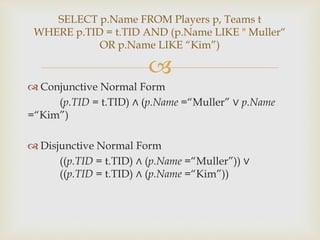
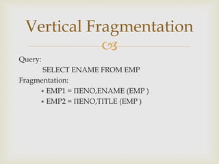
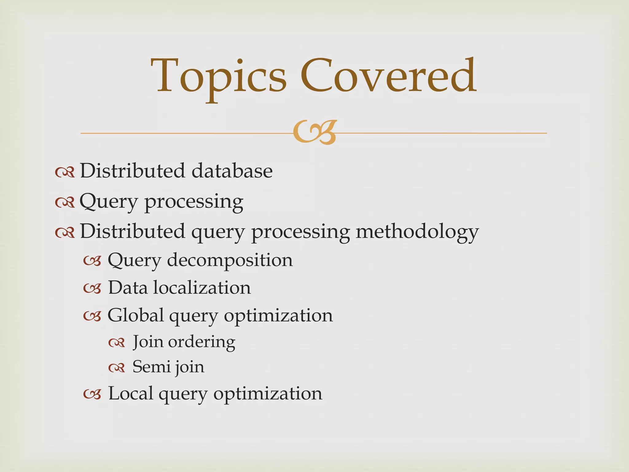
![
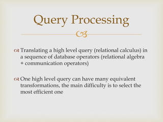
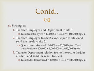
Contd..
3
4
5
7
8
9
A C
R2
A B
1
2
4
5
3 6
R1
Site 1
Site 2
1
2
3
R1[A]
projection
Ship(3)
qs
Ship(2)
Ship(6)
3 7
R2’
reduc
e](https://image.slidesharecdn.com/presentation-150308061527-conversion-gate01/85/Distributed-Query-Processing-27-320.jpg)


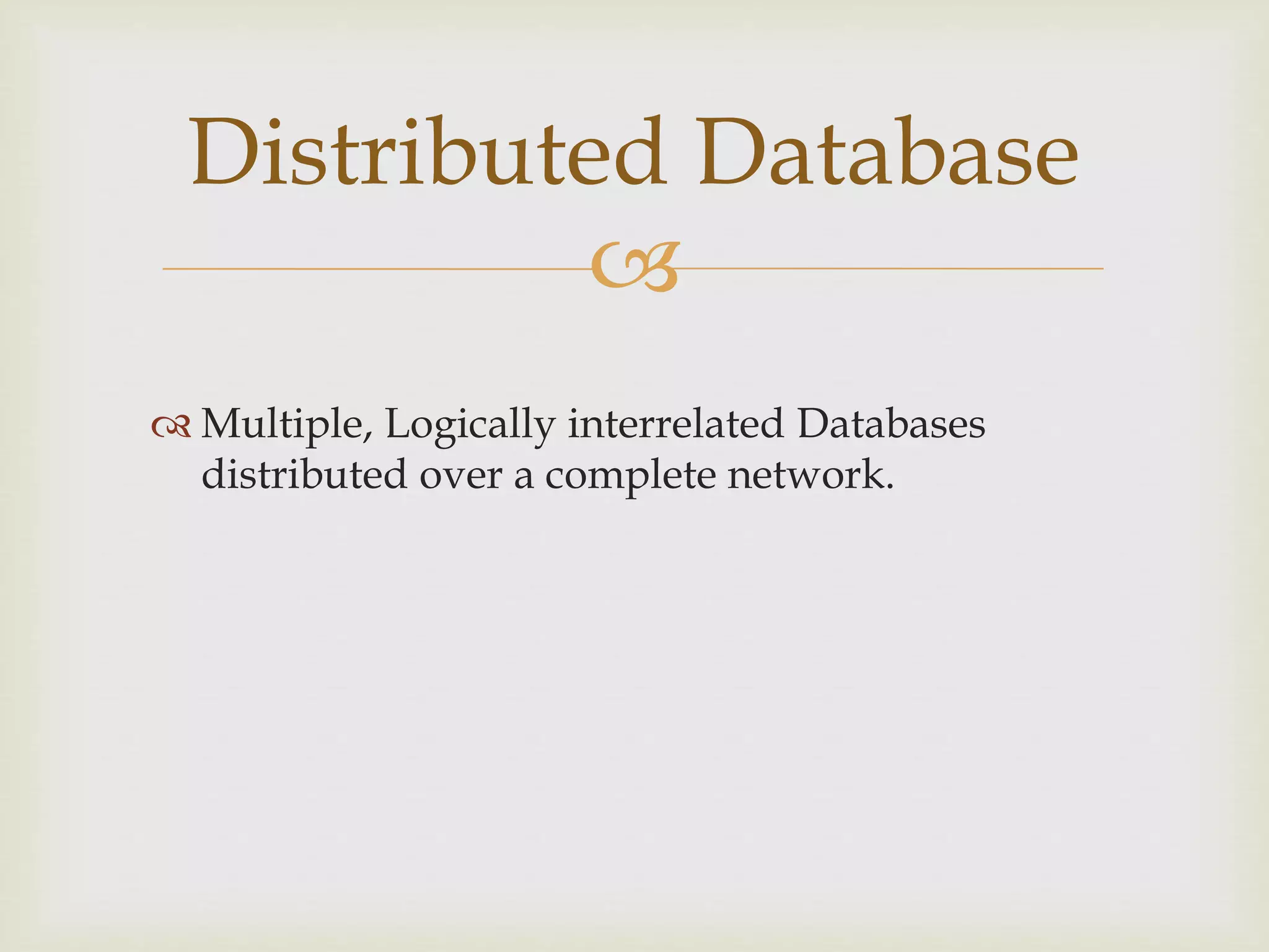


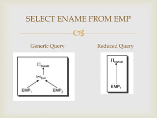
![
It is used to reduce the data transmission cost.
Computing steps:
1) Project Ri on attribute A (Ri[A] ) and
ship this projection ( a semijoin
projection) from the site of Ri to the site
of Rj ;
2) Reduce Rj to Rj’ by eliminating tuples
where attribute A are not matching any
value in Ri[A] .
Semijoin Rj⋉ Ri](https://image.slidesharecdn.com/presentation-150308061527-conversion-gate01/75/Distributed-Query-Processing-26-2048.jpg)
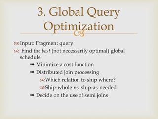
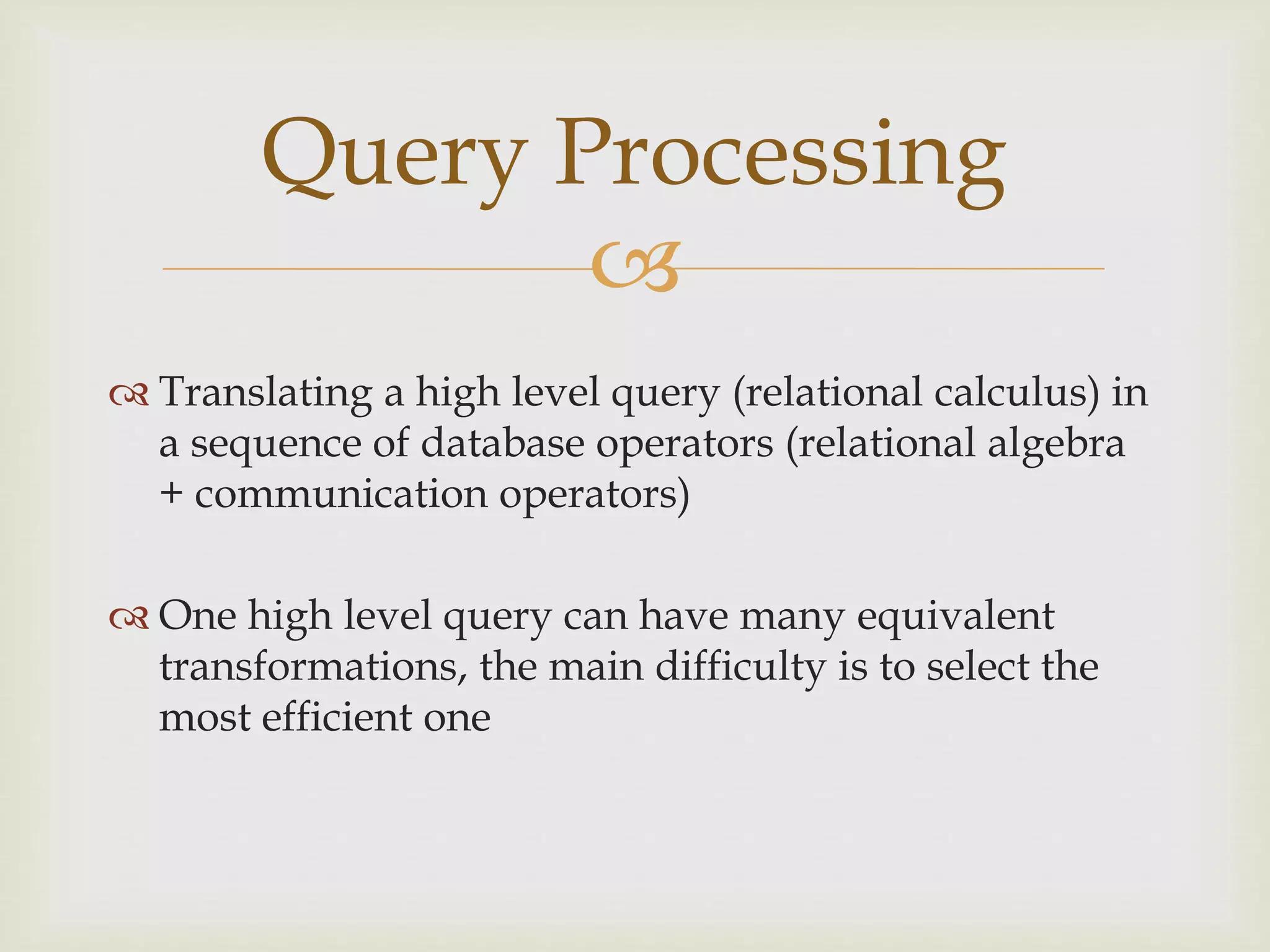
![
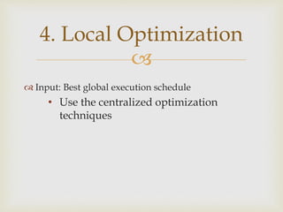
Contd..
3
4
5
7
8
9
A C
R2
A B
1
2
4
5
3 6
R1
Site 1
Site 2
1
2
3
R1[A]
projection
Ship(3)
qs
Ship(2)
Ship(6)
3 7
R2’
reduc
e](https://image.slidesharecdn.com/presentation-150308061527-conversion-gate01/75/Distributed-Query-Processing-27-2048.jpg)


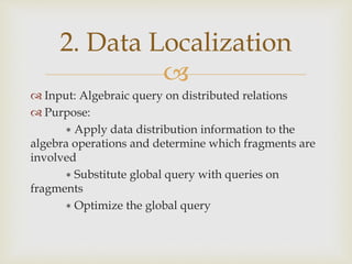
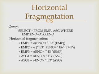
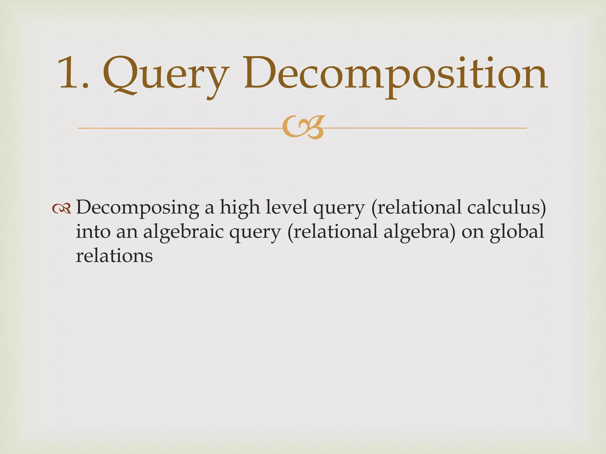
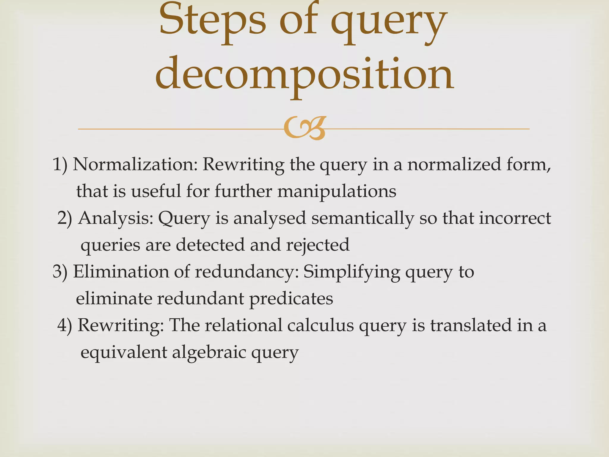
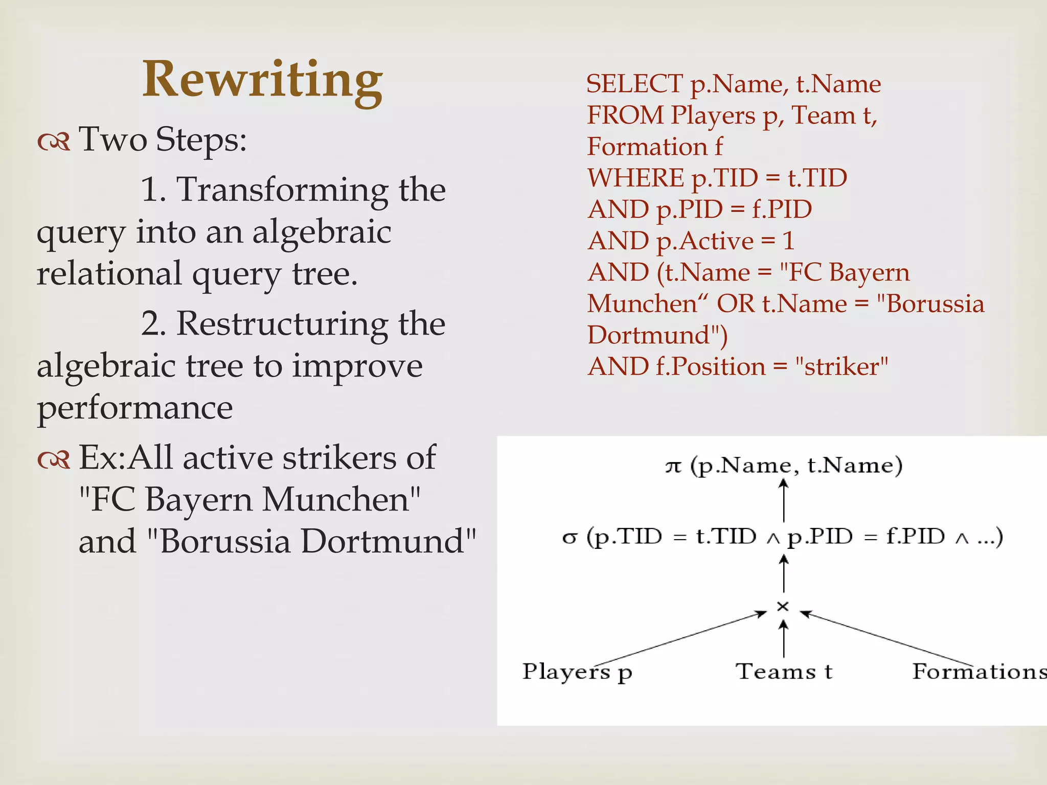
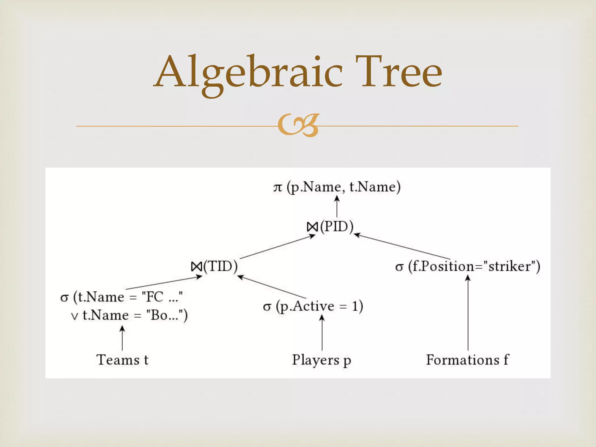
This document discusses distributed database and distributed query processing. It covers topics like distributed database, query processing, distributed query processing methodology including query decomposition, data localization, and global query optimization. Query decomposition involves normalizing, analyzing, eliminating redundancy, and rewriting queries. Data localization applies data distribution to algebraic operations to determine involved fragments. Global query optimization finds the best global schedule to minimize costs and uses techniques like join ordering and semi joins. Local query optimization applies centralized optimization techniques to the best global execution schedule.


